A Multi-population Approach to Forecasting All-Cause Mortality Using Cause-of-Death Mortality Data

Abstract

All-cause mortality is driven by various types of cause-specific mortality. Projecting all-cause mortality based on cause-of-death mortality allows one to understand the drivers of the recent changes in all-cause mortality. However, the existing literature has argued that all-cause mortality projections based on cause-specific mortality experience have a number of serious drawbacks, including the inferior cause-of-death mortality data and the complex dependence structure between causes of death. In this article, we use the recent World Health Organization causes-of-death data to address this issue in a multipopulation context. We construct a new model in the spirit of N. Li and Lee (2005) but in terms of cause-specific mortality. A new two-step beta convergence test is used to capture the cause-specific mortality dynamics between different countries and between different causes. We show that the all-cause mortality estimations produced by the new model perform in the sample similarly to the estimations by the Lee-Carter and Li-Lee all-cause mortality models. However, in contrast to results from earlier studies, we find that the all-cause mortality projections of the new model have better out-of-sample performance in a long forecast horizon. Moreover, for the case of The Netherlands, an approximately 1-year higher remaining life expectancy projection for a 67-year-old Dutch male in a 30-year forecast horizon is obtained by this new model, compared to the all-cause Li-Lee mortality model.

1. INTRODUCTION

Ongoing increases in life expectancy have attracted substantial attention in recent years. The uncertainty around these increases is a concern to social security authorities and pension industries. Several stochastic mortality models have been developed to quantify longevity risk. Among these models, the Lee-Carter (all-cause mortality) model (henceforth the LC model) is regarded as the benchmark method (Booth et al. 2006). Since its appearance in 1992, the literature has expanded in various directions, including cohort effects (Cairns, Blake, and Dowd 2006; Renshaw and Haberman 2006) and developing multipopulation approaches aimed at avoiding diverging projected mortality rates in similar populations (Tuljapurkar, N.Li, and Boe 2000; Li and Lee 2005). These approaches have not yet taken into account causes-of-death information. An alternative approach that has been considered in the literature is to construct all-cause mortality projections based on cause-specific mortality experience. Though some literature states the merits of mortality forecasts based on cause-of-death mortality data (Tabeau et al. 1999), several studies have discussed potential drawbacks of this approach (Wilmoth, 1995; Gutterman and Vanderhoof 1998; Booth and Tickle 2008). The main concerns are inferior data quality and availability, and the complex dependence structure between causes. This article addresses these two issues by modeling cause-specific mortality in a multipopulation context, where the dependence structure will be quantified based on a two-step beta convergence test.

The multipopulation mortality experience has yet not been incorporated in cause-specific mortality modeling to the same extent as in all-cause mortality modeling. Similar decreasing patterns of all-cause mortality among developed countries have been widely illustrated in the literature (Wilmoth, 1998; Wilson, 2001; White, 2002; Janssen 2005). To accommodate this feature in all-cause mortality modeling, N. Li and Lee (2005) extended the LC model to an augmented common factor model that maintains the long-run common trend of the mortality patterns in a group of populations, while allowing for short-run variations in each member of the group. The resulting Li-Lee model produces coherent all-cause mortality forecasts for a group of populations, where “coherence” means that the all-cause mortality forecasts for this group decline at the same speed, maintaining constant interpopulation differences of mortality rates in the long run. N. Li and Lee (2005) attributed this coherence to close links between similar populations in terms of, for example, medical technologies and lifestyles. Generating coherent all-cause mortality forecasts was used by Millossovich et al. (2014) as one of the important criteria to evaluate multi-population mortality models. Moreover, they shed light on the usage of multipopulation mortality models in the assessment of basis risks.

Compared to the coherence of all-cause mortality, the coherence of cause-specific mortality might be easier to identify because the cause-specific driving factors are less confounding than the all-cause factors. For example, all-cause mortality declines are buttressed by many cause-specific medical advances. In addition, fast-growing information and communication technologies help cause-specific medical advances to exchange quickly across borders, potentially leading to a similar speed of decline in cause-specific mortality of developed countries. It has been well documented that mortality rates for cancers (Jemal et al., 2010), vascular diseases (Vallin and Meslé, 2004), and infectious diseases (Omran, 1998) are declining in the United States and other Western countries simultaneously. Therefore, it seems a natural follow-up to model cause-specific mortality in a multipopulation context. Furthermore, to better test cause-specific coherence assumptions, we propose a new “two-step beta convergence test” that is borrowed from the beta convergence approach in the growth literature (Barro, 1991) and in European financial integration studies (Adam et al., 2002). Briefly, the first step is to verify whether the cause-specific mortality rates in different countries are tending to the same level and the second step is to investigate whether these cause-specific mortality rates are tending to improve at the same speed. Using cause-specific multipopulation mortality modeling allows one to avoid the undesired divergence between similar countries in terms of cause-specific mortality forecasts. In addition, for countries with poor causes-of-death mortality records, multipopulation forecasts seem to be more reasonable than those based on single-population mortality histories, because country-specific disturbances are averaged out by extra information incorporated from other similar countries.

Causes of death are usually correlated with each other. The dependence structure between causes plays a pivotal role in modeling cause-specific mortality. Several dependence structures of duration are well studied in the competing risks framework (Carriere, 1994). Yet, the true (net) dependence structure is impossible to identify (Tsiatis, 1975). Honoré and Lleras-Muney (2006) give a famous example of the nonidentifiability problem; that is, the failure in the war on cancer. The well-observed stagnation in cancer mortality declines could be partially explained by a positive dependence between cancer and vascular disease. Both vascular diseases and cancer are positively correlated to some unobserved common risk factors. In the last three decades, innovations in vascular medicines and emergency medical care have reduced the sensitivity of vascular mortality to these common risk factors. As such, the relative risk exposure of cancer has increased because individuals who are exposed to these common factors will eventually die of one cause, either cancer or vascular disease (assuming that these are the only two causes of death). Moreover, the decrease in vascular mortality is more beneficial to individuals with a higher common risk exposure, who are more likely to die from cancer. An individual’s exposure to vascular disease is substituted by the exposure to cancer. Consequently, the mortality declines for cancer are partially masked by such a substitution effect. More recently, copulas have been used to recover the latent cancer mortality declines from observed ones, net of such substitution effects (see Kaishev, Dimitrova, and Haberman 2007; Dimitrova, Haberman, and Kaishev 2013). However, further assumptions, such as the functional forms of copulas and the choice of dependence parameter(s), are needed when using these copula-related models in practice.

Additional assumptions on the dependence structure between causes of death have to be made to utilize cause-specific mortality in all-cause mortality projections. The independence assumption between causes of death is most widely used (see Wilmoth, 1995; Putter, Fiocco, and Geskus 2007). Although the independence assumption might not be realistic, it brings tractability to model the cause-specific mortality and still maintains some interesting features of cause-specific mortality patterns. Alternatively, assuming hierarchical Archimedean copulas for the latent cause-specific survival functions, Li and Lu (2019) derived the latent cause-specific mortality from the observed cause-specific mortality and used the LC model to extract the latent mortality changes for each cause. However, the dependence structure between causes of death that they assume—that is, the functional form of the copulas—cannot be identified from the observed cause-specific mortality data, resulting in a substantial amount of model uncertainty. The true development of some cause-specific mortality could possibly be masked by these assumptions. Instead, Honoré and Lleras-Muney (2006) derived semiparametric bounds for cancer mortality to evaluate the true cancer mortality development with fewer assumptions. They discovered that the semiparametric bounds for cancer mortality are fairly tight and suggested much faster mortality declines in cancer than those previously estimated under the independence assumptions.

Unlike the aforementioned competing risks literature that accounts for the dependence between causes by recovering the unobserved cause-specific mortality from observed mortality, Arnold and Sherris (2013) focused directly on the dependence between observed cause-specific mortality. They applied vector error correction models to identify long-run stationary relationships between the observed cause-specific mortality and used these long-run stationary relationships in their forecasts. This resulted in better performance of the observed cause-specific mortality forecasts. Arnold and Sherris (2013) provided cause-specific mortality projections in a single-population context only, which did not exclude possible divergences between the projections of a group of similar countries. In their spirit, we study the observed cause-specific mortality in a multipopulation context. Instead of using a vector error correction model to identify the dependence structure between causes of death, we use the outcomes of the two-step beta convergence test to model the co-movements between causes of death both in mortality level and in mortality changes, embedding the intercause co-movement in a cause-specific multi-population model, and deriving the mortality implications of the intercause dynamics on all-cause mortality. We incorporate both international dynamics and intercause dynamics in our multipopulation cause-specific mortality models. We introduce two new models, namely, a model that only accounts for cause-specific international dynamics (which we shall refer to as the CoDLi-Lee model) and a model that accounts for both international dynamics and intercause dynamics, based on the outcomes of the two-step beta convergence test (which we shall refer to as the nestedCoDLi-Lee model). We compare these two new models to the traditional all-cause mortality models, namely, the Lee-Carter and the Li-Lee model. We find that the nestedCoDLi-Lee model has a comparable in-sample fit but better out-of-sample performance in a long (i.e., more than 12 years) forecast horizon than the conventional all-cause mortality models.

The rest of our article is organized as follows. Section 2 introduces the data and stylized facts on cause-specific international coherence. Section 3 presents the two-step beta convergence test, including its application to cause-specific international coherence and intercause coherence. Section 4 presents the new cause-specific models. Section 5 discusses the comparison of the in-sample fit and the out-of-sample performance between the aforementioned two models and the conventional all-cause mortality models. Section 6 concludes. Auxiliary graphs and some additional information are presented in the Appendix.

2. DATA AND STYLIZED FACTS

In this section, we introduce the causes-of-death data used in our study and discuss some advantages and disadvantages of using these data. Based on these data, we derive some stylized facts on the international coherence in cause-specific mortality among three countries, which motivates our two-step beta convergence test in the next section.

2.1. Data

According to the International Classification of Diseases (ICD) in WHO (2018a), the definition of a cause of death is “the disease or injury which initiated the train of morbid events leading directly to death, or the circumstances of the accident or violence which produced the fatal injury.” A compilation of mortality data in WHO (2018b) by age, sex, and causes of death from 1979 to 2015 is provided by the World Health Organization (WHO). The access version of this database is used here, which features the consistent causes of death data collected officially by the WHO from countries that are using the newest ICD-9 and ICD-10 and data on population and live births. Through these features, we ensure fewer discontinuities caused by changes in ICD versions as indicated by Gaille and Sherris (2011). The cause-specific mortality trends estimated and projected via this database are hence more robust to the evolution of ICD in different countries and different time periods.

The disadvantages of this database, however, are also obvious. First, the age groups are relatively large; that is, 0, 1–4, 5–14, 15–24, 25–34, 35–54, 55–74, 75+. Although other causes-of-death datasets might contain smaller age groups, like the one used in Arnold and Sherris (2013), who use 5-year age groups, these alternatives originate from the WHO query version data that require the users to update the ICD regularly. Most important users of these alternative datasets have to use smoothing techniques to level off discontinuities caused by updates to the ICD. This data maneuvering well documented in Arnold and Sherris (2013). To what extent the underlying trends of causes-of-death mortality may be affected by these smoothing techniques is an open question. In this sense, we prefer the WHO access version data with its larger age groups, to preserve the underlying causes-of-death mortality dynamics between different countries and different causes. Second, to cope with the new ICD versions, few developed countries have full records of long enough mortality histories for all important causes of death.¹

From the aforementioned data, we use the cause-specific number of deaths and the corresponding number of exposures for males, age groups (25–34, 35–54, 55–74, 75+),² and time period (1979–2013) in The Netherlands (NL), Belgium (BE), and France (FR). We define $D_{x,t}^{s,v}$ as the number of deaths of cause s in country v for age group x at time t and let $E_{x,t}^v$ be the all-cause exposure in country v for age group x at time t. Then, the observed cause-specific raw central death rate of cause s in country v for age group x at time t, $m_{x,t}^{s,v},$ is given by (1) $$\begin{array}{c}{m}_{x,t}^{s,v}=\frac{D_{x,t}^{s,v}}{E_{x,t}^v}.\hfill \end{array}$$(1)

The all-cause mortality rate in country v for age group x at time t, $m_{x,t}^v,$ is then given by (2) $$\begin{array}{c}{m}_{x,t}^v=\frac{\sum _s{D}_{x,t}^{s,v}}{E_{x,t}^v}\hfill \end{array},$$(2) where the sum in the numerator is over all causes.

In our case, $t\in \{1979,\dots ,2013\},v\in \{\mathit{The}\mathit{Netherlands},\mathit{France},\mathit{Belgium}\},$ and x refers to the age groups 25–34, 35–54, 55–74, and 75+ years old. All-cause mortality is dis-aggregated into five main causes of death; that is, cancer (CM), vascular diseases (VM), diseases of other causes (referred as other diseases or DM), accidents and murders (AMM), and the unexplained (UEM). Thus, $s\in \{$CM, DM, VM, AMM, UEM$\}.$ Table 1 shows the coding rules. In line with earlier studies, we chose the most common causes in developed countries. For instance, cancer, diseases of the circulatory system, and other diseases we considered by Boumezoued et al. (2018) as the three main causes in their study. In addition, similar categorizations of causes of death were used in previous studies (Oeppen 2008; Alai, Arnold, and Sherris 2015).

TABLE 1 Coding Rules of Causes of Death (Males)

Cause of death	Abbreviation	ICD chapter
Cancer	CM	2 (Neoplasms)
Vascular disease	VM	9 (Diseases of the circulatory system)
Other diseases	DM	1 (Certain infectious and parasitic diseases)
		4 (Endocrine, nutritional, and metabolic diseases)
		5 (Mental and behavioral disorders)
		6 (Diseases of the nervous system)
		7 (Diseases of the eye and adnexa)
		8 (Diseases of the ear and mastoid process)
		10 (Diseases of the respiratory system)
		11 (Diseases of the digestive system)
		12 (Diseases of the skin and subcutaneous tissue)
		13 (Diseases of the musculoskeletal system and connective tissue)
		14 (Diseases of the genitourinary system)
		17 (Congenital malformations, deformations, and abnormalities)
Accidents and murders	AMM	20 (External causes of morbidity and mortality)
Unexplained	UEM	15 (Pregnancy, childbirth, and the puerperium)
		16 (Conditions originating in the perinatal period)
		18 (Symptoms, signs, and abnormal clinical and laboratory findings)

2.2. Stylized Facts

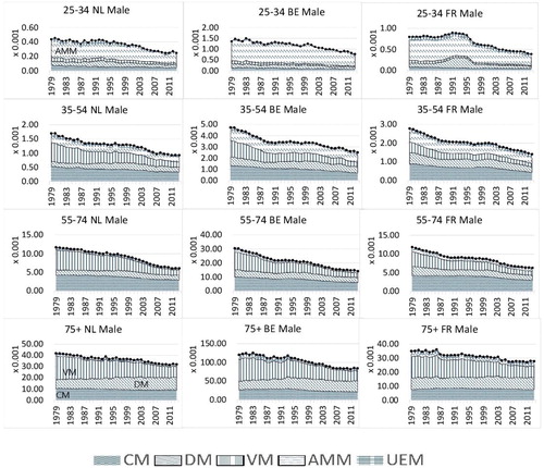
We show the past trends of the causes-of-death mortality in Figure 1 for the different age groups and the three countries in terms of mortality component graphs. For the age group 25–34, there is a jump in the central mortality rate for other diseases (DM) in the 1990s in France. This is the result of a relatively widespread epidemic of influenza-like illness at that time; see Carrat et al. (1998). The attack rate was highest among young people and decreased with increasing age. Therefore, there is little sign of such an epidemic in the older age groups in France. We do not see a similar jump in The Netherlands and Belgium, implying that a common mortality trend of other diseases (DM) in these three countries might be insensitive to this country-specific epidemic. Among the younger age groups (25–34 and 35–54; first and second rows), accidents and murders (AMM), including external injuries, were also a major cause of death in the three countries. This stylized fact is in line with the findings for European countries in Mathers et al. (2009). For the elderly age groups (55–74 and 75+) in these three countries (third and fourth rows), we observe smoother patterns of causes-of-death mortality trends than those for younger age groups. The vascular revolution since the 1970s can be seen as the decreasing proportions of vascular diseases (VM) from 1979 to 2013 in the mortality component graphs, mainly appearing in the age groups over 35–54 years old. Moreover, echoing Bongaarts (2014), the cancer phase mortality transition of high-technology societies began in some developed countries in the mid-1990s, which is evident for the age groups 35–54 and 55–74 for all three countries. This implies that cancer mortality might decrease at a slower pace initially but might decline faster if the transition is nearing the end in the future. In order to take a closer look at certain important causes of death—for example, cancer and vascular diseases—we summarize the stylized facts on causes-of-death dynamics among the three countries in terms of the age-adjusted cause-specific mortality rates (ss Arnold and Sherris 2013).

Figure 1. Mortality Component Graph for NL, BE, and FR.

2.2.1. Mortality Level

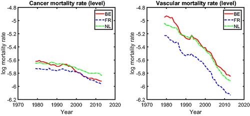
In Figure 2, we present the mortality rates for CM (left panel) and VM (right panel). The left panel shows that for most periods, cancer mortality in the three countries behaves similarly, except for the period 1995–2005. We observe a catch-up effect among these three countries during this period; that is, the cancer mortality in Belgium (solid line) initially starts to decline at a significantly faster pace around 1995, followed later by France (dashed line) and The Netherlands (dashed-dotted line). After 2005, cancer mortality in these three countries behaves similarly again. The right panel of Figure 2 indicates that the vascular mortality rates in The Netherlands, Belgium, and France improve at a similar pace. Visual inspection of Figure 2 thus suggests international coherence in cancer and vascular mortality; that is, mortality in similar countries’ changes at the same speed in the long run (after catching up), defining coherence similar to Li and Lee (2005).³ The phenomena observed in Figure 2 are in line with the findings of Bremberg (2017). He showed that there exists a significant catch-up effect in the all-cause mortality rates among 55- to 75-year-olds in Organization for Economic Cooperation and Development countries; that is, the gap between the speed of mortality changes in all-cause mortality in Organization for Economic Cooperation and Development countries has decreased since the 1990s. Faster dissemination of medical innovations during the 1990s, fueled by the booming of information technologies, is believed to be one of the main drivers. We provide a natural follow-up on whether cause-specific mortality changes echo this story.

Figure 2. Cancer and Vascular Mortality Rate.

2.2.2. Mortality Changes

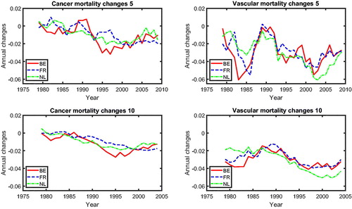
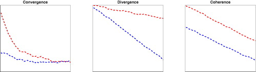
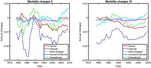
Figure 3 shows the mortality changes corresponding to the mortality rates presented in Figure 2. The mortality changes are estimated via a 5-year rolling window or a 10-year rolling window.⁴ We observe that cancer and vascular mortality in Belgium, The Netherlands, and France are improving roughly at the same speed. We observe converging cancer and vascular mortality changes in the three countries using both the 5-year rolling window and the 10-year rolling window.⁵ In order to identify the type of co-movements between the mortality rates, we introduce a new test-based procedure in the next section.

Figure 3. Cancer and Vascular Mortality Changes in Different Rolling Windows.

3. TWO-STEP BETA CONVERGENCE TEST

Inspired by the empirical results on international coherence in Section 2.2, we introduce a new test-based procedure to pin down group memberships for this international coherence, in order to utilize these memberships in a Li-Lee framework. As alternatives, there are several ways to determine the coherence membership. One possibility is the original way proposed by N. Li and Lee (2005), who tested whether the member-specific period effect in the second stage (after removing the common period effect in a first stage) is stationary or not.⁶ The other was proposed by Hatzopoulos and Haberman (2013), who determined coherence memberships using a generalized linear model framework.

As pointed out by N. Li and Lee (2005), the definition of a coherent group is intentionally vague, because some countries that are going through a transitory period of mortality—for example, eastern European Union countries—could also be included in a group with Western European Union countries, even though the country-specific period effects might not satisfy the stationarity assumption. However, the definition in terms of stationarity of member-specific period effects might also rule out some countries whose inclusion in a coherent group seems plausible. For example, Hatzopoulos and Haberman (2013) showed that Scotland is excluded from the coherent group of male mortality in Western Europe when using the Li-Lee method to determine group membership. Apparently, Scotland is not a country that is in a transitory period and is arguably similar to England and Wales in socioeconomic status. To deal with such a dilemma, a more precise way to define the membership of a coherent group is needed.

Unlike Hatzopoulos and Haberman (2013), who determined the coherent membership of a country via the coefficients of a rather complicated dynamic linear regression, we propose to determine the coherence membership within the Li-Lee model with a two-step beta convergence test. We first describe this two-step beta convergence test, after which we establish the link between this test and the Li-Lee model.

3.1. Two-Step Beta Convergence Test and Its Link to the Li-Lee Model

The two-step beta convergence test is built on the one-step beta convergence test proposed by Barro (1991). For similar applications in mortality studies, d’Albis, Esso, and Pifarré i Arolas (2012) introduced a single-step beta convergence test to test convergence in mortality rates. The beta convergence test is originally used to check whether a negative relationship exists between the gross domestic product growth rate and its initial level. In our case, we replace gross domestic product growth with mortality changes. More specifically, we want to investigate whether the mortality rate would decline faster (slower) when the mortality rate is at a relatively high (low) level or whether there is a catch-up effect in mortality rates between different countries. This means that different countries or different causes of death are heading toward the same mortality level in the long run. Moreover, we not only test for convergence in the mortality levels but we also test for convergence in mortality changes. Convergence in mortality changes means that mortality changes in different countries tend toward a constant in the long run; that is, the considered countries share the same mortality changes.

3.1.1. First Step: Beta Convergence Test in Mortality Level

Let $d{m}_{x,t}^v=\log (m_{x,t+k}^v)-\log (m_{x,t}^v)$ represent the k rolling window mortality changes for age x, time t, and country v. Consider the following regression equation: (3) $$\begin{array}{c}d{m}_{x,t}^v={\alpha }_v+{\beta }_{\text{level}}\hspace{0.17em}\text{log}\hspace{0.17em}(m_{x,t}^v)+\sum _{l=1}^L{\gamma }_{l}d{m}_{x,t-l}^v+{\epsilon }_{x,t}^v,v\in \{\mathit{Netherlands},\mathit{France},\mathit{Belgium}\}.\hfill \end{array}$$(3)

In this equation, α_v is the country-specific effect, β_level quantifies the relation between the mortality changes and its initial mortality level, and γ_l are the coefficients of the lagged terms, which control for past information and deal with the autocorrelation in error terms. The error terms ${\epsilon }_{x,t}^v$ are assumed to satisfy the usual regression assumptions.⁷

The key coefficient is β_level. A negative value of β_level corresponds to convergence in the mortality level (type 1 co-movement in Figure 4); a positive value of β_level corresponds to a divergence in the mortality level (type 2 co-movement in Figure 4). Thus, a significant negative β_level (for example, at a two-sided 5% significance level) indicates convergence in the mortality level, whereas a significant positive β_level indicates divergence in the mortality level. If β_level is not significantly different from 0, there is no clear link between mortality changes and its initial mortality level.

Figure 4. Co-Movement Types. Note: Left to right: Type 1 convergence, type 2 divergence, type 3 coherence.

The results of the beta convergence test will be sensitive to the choice of the length k of the rolling window in $d{m}_{x,t}^v.$ This is due to a trade-off between bias and efficiency. There will be more noise in the estimated mortality changes with a shorter rolling window length, which might negatively affect the efficiency of the results. The degree of noise can be reduced by extending the rolling window, but then the results may become more biased due to potential misspecification when using a longer rolling window length. This is a typical bias–efficiency trade-off. We therefore present the results for different rolling window lengths (k).

To guarantee coherent mortality forecasts—that is, that members of a coherent group would not have a diverging mortality forecast in the long run—either type 1 convergence or type 3 coherence (see Figure 4) should be present. Because type 1 convergence will already be pointed out by the negative β_level, we need an extra indicator for type 3 coherence. Therefore, we propose an additional step to be discussed next.

3.1.2. Second Step: Beta Convergence Test in Mortality Changes

Let $\Delta d{m}_{x,t}^v=d{m}_{x,t+1}^v-d{m}_{x,t}^v$ represent the difference in mortality changes between time t and the next period, for age x and country v. Consider the following regression equation, which is the same as Equation (3)(3) $$\begin{array}{c}d{m}_{x,t}^v={\alpha }_v+{\beta }_{\text{level}}\hspace{0.17em}\text{log}\hspace{0.17em}(m_{x,t}^v)+\sum _{l=1}^L{\gamma }_{l}d{m}_{x,t-l}^v+{\epsilon }_{x,t}^v,v\in \{\mathit{Netherlands},\mathit{France},\mathit{Belgium}\}.\hfill \end{array}$$(3) but with $d{m}_{x,t}^v$ replaced by $\Delta d{m}_{x,t}^v:$ (4) $$\begin{array}{c}\Delta d{m}_{x,t}^v={\alpha }_v+{\beta }_{\text{trend}}d{m}_{x,t}^v+\sum _{l=1}^L{\gamma }_l\Delta d{m}_{x,t-l}^v+{\epsilon }_{x,t}^v,v\in \{\mathit{Netherlands},\mathit{France},\mathit{Belgium}\}.\hfill \end{array}$$(4)

We apply the beta convergence test of Equation (3)(3) $$\begin{array}{c}d{m}_{x,t}^v={\alpha }_v+{\beta }_{\text{level}}\hspace{0.17em}\text{log}\hspace{0.17em}(m_{x,t}^v)+\sum _{l=1}^L{\gamma }_{l}d{m}_{x,t-l}^v+{\epsilon }_{x,t}^v,v\in \{\mathit{Netherlands},\mathit{France},\mathit{Belgium}\}.\hfill \end{array}$$(3) again, but now in terms of mortality changes. The interpretation of the parameters of the models remains the same. The key coefficient is now β_trend. A significant (two-sided 5% significance level) negative β_trend would indicate convergence in mortality changes; that is, the coherence in mortality levels (type 3 co-movement, coherence; see Figure 4).

3.1.3. Link β_level and β_trend to Li-Lee Model

The two-step beta convergence test aims to determine the co-movement types (convergence, divergence, or coherence) of a group of time series processes. For a country to be included in a coherent group in the Li-Lee model, it is required that the mortality pattern of this country should not diverge from those of other members in the coherent group. We use the two-step beta convergence test to determine whether convergence, divergence, or coherence in the cause-specific mortality trajectories of a group of countries exists to determine which country should be included in the Li-Lee model. In addition, we translate the coefficients of the two-step beta convergence test β_level and β_trend to the model specifications of the Li-Lee model.

Let us first briefly review the Li-Lee model: (5) $$\begin{array}{c}\hspace{0.17em}\text{ln}\hspace{0.17em}(m_{x,t}^v)={\alpha }_x^v+B_x{K}_t+b_x^v{k}_t^v+{\epsilon }_{x,t}^v.\hfill \end{array}$$(5)

Here, $a_x^v$ is the age effect. To prevent subpopulations of the group from diverging from each other in the long run, $B_x{K}_t$ is the common factor for each country in the group. K_t is the common period effect and B_x is the common sensitivity of age x to this common period effect. To allow for short-run variations of subpopulations of the group, $b_x^v{k}_t^v$ is the individual factor of country v that is supposed to vanish in the long run. $k_t^v$ is the individual period effect and $b_x^v$ is the sensitivity of age x to the individual period effect. The typical normalizations are $\sum _x{B}_x=1,\sum _t{K}_t=0,\sum _x{b}_x^v=1,$ and $\sum _x{k}_t^v=0.$ We estimate the Li-Lee model via singular value decomposition (SVD) in two steps (N. Li and Lee, 2005). For the common period effect K_t, a random walk with drift (RWD) process is commonly selected ⁸; that is, $K_t=B_0+K_{t-1}+e_t.$ Specifically, B₀ is the drift term of the RWD process and e_t is the random variable with an independent and identically distributed (i.i.d.) normal distribution across time. For the country-specific period effect $k_t^v,$ N. Li and Lee (2005) suggested keeping the population v in the coherent group if the explanation ratio⁹ of the augmented common factor model is large enough and $k_t^v$ could be well described by a stationary process, such as an AR(1) process—that is, $k_t^v={\beta }_0^v+{\beta }_1^v{k}_{t-1}^v+u_t^v$—in which ${\beta }_1^v$ is required to be less than one (in absolute value).

In our approach, whether a country should be included in a coherent group or not will be determined by the value of β_level and β_trend of the two-step beta convergence test. First, we utilize the results of the two-step beta convergence test on $m_{x,t}^v$ to profile the characteristics of the common period effect K_t and the country-specific period effect $k_t^v.$ Second, we select the countries whose $k_t^v$ is stationary in a coherent group. Third, as suggested by N. Li and Lee (2005), we re-estimate K_t and $k_t^v$ based on a refined coherent group of countries. Subsequently, we use the re-estimated K_t and $k_t^v$ to generate the mortality forecasts.

Table 2 summarizes the relevant links between the two-step beta convergence test and the Li-Lee model. If ${\beta }_{\text{level}}<0$ and ${\beta }_{\text{trend}}<0,$ this indicates that the mortality levels of different countries are tending toward the same value, as are the mortality changes. If this tendency were to continue in the projections, the mortality levels and mortality changes of the different countries would be the same in the long run. This long-run interplay between the different countries in mortality levels and mortality changes could be characterized by the Li-Lee model with a K_t that is modeled as a RWD and $k_t^v$ that are modeled (for example) as AR(1) processes.

Table 2 Two-Step Beta Convergence Test and Its Link to Li-Lee Model^a

First step	Second step	Li-Lee model	Co-movement type at steady⋯
${\beta }_{\text{level}}<0$	${\beta }_{\text{trend}}<0$	Li-Lee RWD(1) + ARIMA(1, 0, 0)	Convergence
${\beta }_{\text{level}}>0$	${\beta }_{\text{trend}}=0$	Li-Lee RWD(1) + ARIMA(0, 1, 0)	Divergence
${\beta }_{\text{level}}>0$	${\beta }_{\text{trend}}>0$	Li-Lee RWD(1) + nonstationary ARIMA (1, 1, 0)	Divergence
${\beta }_{\text{level}}=0$	${\beta }_{\text{trend}}<0$	Li-Lee RWD(1) + AR(1) or Li-Lee RWD(1) + stationary ARIMA(1, 1, 0)	Coherence

^a This table summarizes the link between the results of the two-step beta convergence test and the Li-Lee model. The test captures the dynamics between mortality patterns of different countries in the sample data. ARIMA = autoregressive integrated moving average.

If ${\beta }_{\text{level}}>0$ and ${\beta }_{\text{trend}}=0,$ this shows that the mortality levels in different countries are tending toward different values and there is no clear tendency in the mortality changes. Were this tendency to continue in the projections, the mortality levels of the different countries would diverge in the long run. This long-run interplay could be characterized by the Li-Lee model with both K_t and $k_t^v$ as RWD; that is, ARIMA(0, 1, 0).

If ${\beta }_{\text{level}}>0$ and ${\beta }_{\text{trend}}>0,$ this suggests that the mortality levels in the different countries are tending toward different values and so are the mortality changes. Were this tendency to continue in the projections, the mortality levels and the mortality changes in the different countries would diverge in the long run. This long-run co-movement between different countries could be captured by the Li-Lee model with a K_t that is modeled as an RWD and the $k_t^v$ that are modeled as nonstationary processes, such as ARIMA(1, 1, 0) (see Eq. [B.11](B.11) $$\begin{array}{cc}\underset{T_L\to \infty }{\lim }\mathbb{E}(\hspace{0.17em}\text{log}\hspace{0.17em}(m_{x,t+T_L}^v))-\mathbb{E}(\hspace{0.17em}\text{log}\hspace{0.17em}(m_{x,t+T_L}^{v\prime }))\hfill & ={\alpha }_x^v-{\alpha }_x^{v\prime }+[\frac{1}{1-{\beta }_1^v}{k}_t^v-\frac{{\beta }_1^v}{1-{\beta }_1^v}{k}_{t-1}^v]\hfill \\ \hfill & -[\frac{1}{1-{\beta }_1^{v\prime }}{k}_t^{v\prime }-\frac{{\beta }_1^v}{1-{\beta }_1^{v\prime }}{k}_{t-1}^{v\prime }].\hfill \end{array}$$(B.11) in the Appendix).

If ${\beta }_{\text{level}}=0$ and ${\beta }_{\text{trend}}<0,$ this suggests that the mortality changes in the different countries tend toward the same value. Were this tendency to continue in the projections, the mortality changes in the different countries would converge in the long run. Such long-run co-movements between different countries could be captured by the Li-Lee model with a K_t that is modeled as an RWD and the $k_t^v$ that are modeled by an AR(1) process or by an ARIMA(1, 1, 0).

We only present the case in which all countries in a coherent group share the same type of time series processes; for example, all cause-specific period effects are AR(1) processes. In the Appendix we discuss the case where one country could have an AR(1) process and the other country could have an ARIMA(1, 1, 0) process. But the main results do not change much if we have a stationary AR component in the country-specific period effect $k_t^v,$ no matter whether $k_t^v$ follows an ARIMA(1,1,0) or AR(1) process. We rule out the impossible scenarios at the steady state—for example, ${\beta }_{\text{level}}<0$ and ${\beta }_{\text{trend}}>0$—because if the mortality levels in different countries converge to the same value in the steady state, their mortality changes should also be equal. In addition, we rule out the cases in which there exist two identical country-specific factors for two different countries; that is, we impose $b_x^v{\beta }_0^v\ne b_x^{v\prime }{\beta }_0^{v\prime },v\ne v\prime ,v,v\prime \in \{NL,BE,FR\}.$

We utilize the two-step beta convergence test in Subsections 3.2 and 3.3 to determine whether international coherence and intercause coherence, respectively, exist. Subsequently, we construct the optimal group memberships of international coherence.

3.2. Application of Two-Step Beta Convergence Test: International Comparison

In this section, we apply the two-step beta convergence test to cause-specific mortality across the three countries. We present the results for age-adjusted cause-specific mortality. The results for the individual age classes are quite similar. Figure 5 shows β_level (left panels) and β_trend (right panels) for cancer (upper panels) and vascular mortality (lower panels). Figure 6 shows the corresponding p values, using the same format. The left panels of Figure 5 show that β_level of cancer mortality is negative for most rolling window choices, whereas that for vascular mortality is fluctuating around zero. However, both are insignificant at the double-sided 5% level for all rolling window choices, according to the left panels of Figure 6. This means that the mortality changes are not significantly related to the initial mortality level; that is, $H_0:{\beta }_{\text{level}}=0$ cannot be rejected, meaning that there is no sign of convergence or divergence in mortality level. On the contrary, the right panels of Figure 5 suggest that β_trend for both cancer and vascular mortality are negative. Moreover, the right panels of Figure 6 show that the negative β_trend for cancer and vascular mortality is significant at the double-sided 5% level. This indicates that the difference in mortality changes is negatively related to the initial state of the mortality changes; that is, ${\beta }_{\text{trend}}<0,$ indicating convergence in mortality changes.

Figure 5. International Comparison: β_level and β_trend for Cancer and Vascular Mortality.

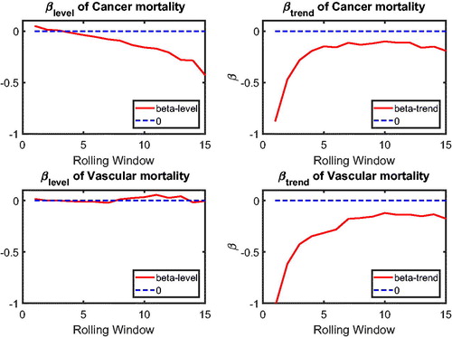
Figure 6. International Comparison: p Value of β_level and β_trend for Cancer and Vascular Mortality.

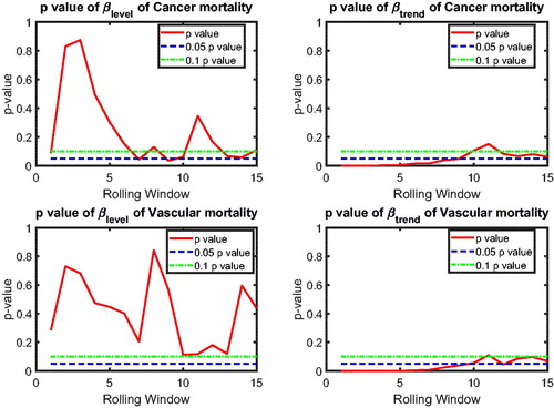
Referring to Table 2, the combination ${\beta }_{\text{level}}=0$ and ${\beta }_{\text{trend}}<0$ indicates that the co-movements between The Netherlands, Belgium, and France are coherent.¹⁰ Figures C.3 and C.4 (in the Appendix) suggest international convergence (type 1) for other diseases, accidents and murders, and the unexplained. In all, no divergent pattern has been found in all cause-specific mortality among these three countries.

3.3. Application of Two-Step Beta Convergence Test: Intercause Comparison

In addition to the international dynamics in cause-specific mortality across the three countries, in this section we provide an inter-cause comparison. This intercause comparison will shed light on possible catch-up effects between the different causes, which could improve the forecasts of a cause that initially improves at a slower speed but catches up with other causes at a faster speed. Take cancer and vascular diseases as an example. Given that vascular mortality is decreasing much faster than cancer mortality, reaching a historically low level, more focus of media coverage and more efforts in medical research might shift from preventing and curing the former to the latter, resulting in a catch-up in the cancer mortality declines. In addition, some medical innovations that apply to vascular mortality could be modified to cure cancer. Recent research on the shared risk factors for vascular diseases and cancer is a step in this direction; see Koene et al. (2016). The catch-up effect between the two causes is expected to be more significant if these two causes are highly correlated, because the higher the correlation the easier the dissemination of medical innovations from one cause to the other cause.

Given that the international coherence in main cause-specific mortality has been supported by the results of Subsection 2.2, let the common cause-specific mortality in The Netherlands, Belgium, and France be given as follows: (6) $$\begin{array}{c}{m}_{x,t}^s=\frac{\sum _v{D}_{x,t}^{s,v}}{\sum _v{E}_{x,t}^v},\hfill \end{array}$$(6) where the sums are over the three countries.

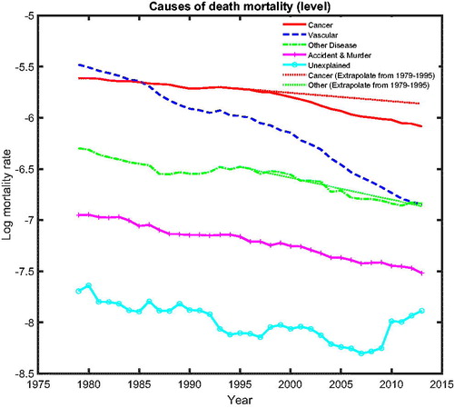
The common cause-specific mortality will be used to examine the inter-cause comparison between the five main causes of death. Figure 7 presents the common cause-specific mortality levels.¹¹ The figure shows that the fastest declining cause of death is vascular mortality. Vascular disease was the most important cause of death in The Netherlands, Belgium, and France but became second to cancer mortality after about 1985. The figure also suggests that cancer mortality decreased faster after the 1990s, whereas other diseases only decreased slightly. We visualize this by comparing simple linear extrapolations based on the period from 1979 to 1995 (dotted line for cancer mortality and dotted line for other diseases), with the realizations from 1996 to 2013 (solid line for cancer mortality and dashed-dotted line for other diseases). For other diseases, the linear extrapolation, based on its speed of mortality decline from 1979 to 1995, closely follows the realizations, suggesting that its speed of mortality decline between 1979 and 1995 was similar to that between 1996 and 2013. However, for cancer, we see that the speed of mortality decline between 1996 and 2013 is faster than that between 1979 and 1995 because the realizations for cancer mortality are below the linear extrapolation. The turning point of cancer mortality declines is roughly 15 years after cancer mortality surpassed vascular mortality and became the most deadly disease. This indicates that there might be a catch-up effect between cancer and vascular mortality, which might be informative for the forecasts of cancer mortality.

Figure 7. Cause-Specific Common Mortality Rate. Note: The additional dotted lines represent the linear extrapolation of the common mortality rate for cancer and other diseases based on the history from 1979 to 1995.

Figure 8 presents the common cause-specific mortality changes for a rolling window of 5 years (left panel) and a rolling window of 15 years (right panel). From this figure, we can observe that mortality changes for cancer and vascular diseases converge to a similar value beginning in the 1990s, suggesting a possible cancer–vascular disease coherence, whereas other diseases fluctuate below zero but above cancer, which is in line with the results for mortality level (see Figure 7).

Figure 8. Cause-Specific Mortality Changes in Different Rolling Windows.

Following similar logic as in Subsection 3.2, in this subsection, we apply the two-step beta convergence test to the mortality levels of the intercause comparison, (7) $$\begin{array}{c}d{m}_{x,t}^s={\alpha }_s+{\beta }_{\text{level}}{\text{log}m}_{x,t}^s+\sum _{l=1}^L{\gamma }_{l}d{m}_{x,t-1}^s+{\epsilon }_{x,t}^s,s\in \{CM,DM,VM,\mathit{AMM},\mathit{UEM}\},\hfill \end{array}$$(7) and to the mortality changes of the intercause comparison (8) $$\begin{array}{c}\Delta d{m}_{x,t}^s={\alpha }_s+{\beta }_{\text{slope}}d{m}_{x,t}^s+\sum _{l=1}^L{\gamma }_l\Delta d{m}_{x,t}^s+{\epsilon }_{x,t}^s,s\in \{CM,DM,VM,\mathit{AMM},\mathit{UEM}\},\hfill \end{array}$$(8) to test intercause coherence. Via the two-step beta convergence test, we obtain the results presented in Table 3. This table shows the implied co-movement types between the causes of death. One pitfall in the results for intercause coherence is that other diseases might not be coherent to AMM because their correlation is weak. However, the coherence suggested by the test outcome might result from the fact that both of these causes are relatively more stationary (see Figure 8) compared to vascular mortality, which decreased dramatically.

Table 3 Intercause Two-Step Beta Convergence Test Results

Intercause	Co-movement type	Figure
Cancer–vascular disease	Coherence	Figure C.5
Cancer–other diseases	No coherence	Figure C.6
Cancer–accidents and murders	No coherence	Figure C.7
Cancer–unexplained	No coherence	Figure C.8
Vascular disease–other diseases	No coherence	Figure C.9
Vascular disease–accidents and murders	No coherence	Figure C.10
Vascular–unexplained	No coherence	Figure C.11
Other diseases–accidents and murders	Coherence	Figure C.12
Other diseases–unexplained	No coherence	Figure C.13
Accidents and murders–unexplained	No coherence	Figure C.14

Based on the two-step beta convergence test, we find that there only exists cancer–vascular disease coherence and other disease-accidents and murder coherence, which is consistent with the data visualization in Figures 7 and Figure 8.¹² In the following sections, we incorporate the intercause coherence and the aforementioned international coherence in a new nestedCoDLi-Lee model.

4. MODELS

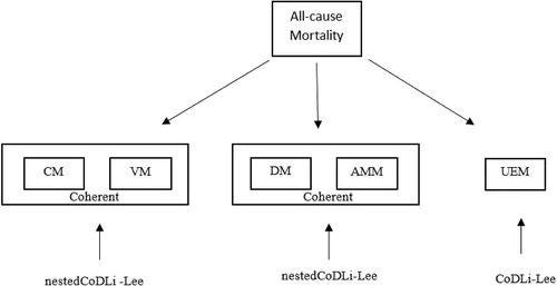
In this section, we introduce two types of mortality models. One type consists of all-cause mortality models that are based on all-cause mortality, including the all-cause Lee-Carter model and the already introduced all-cause Li-Lee model. The other type consists of cause-specific mortality models that are based on cause-specific mortality, including a causes-of-death Lee-Carter model (referred to as CoDLC, not presented¹³); a causes-of-death Li-Lee model (referred to as CoDLi-Lee), which only accounts for cause-specific international coherence; and a nested causes-of-death Li-Lee model (referred to as nestedCoDLi-Lee) that accounts for both international coherence and intercause coherence as suggested by the two-step beta convergence test. In order to avoid introducing too much noise, we do not make use of a Li-Lee model at the most disaggregated mortality level; that is, the country–cause level. Instead, we make use of a nested model in the spirit of Li-Lee, which, due to less disaggregation, will be less sensitive to possible noisy country–cause combinations.

4.1. All-Cause Mortality Models

In this subsection we only present the all-cause Lee-Carter model, because we already introduced the all-cause Li-Lee model. The Lee-Carter model is applied to all-cause mortality and is defined as follows: (9) $$\begin{array}{c}\hspace{0.17em}\text{ln}\hspace{0.17em}(m_{x,t}^v)={\alpha }_x^v+B_x^v{K}_t^v+{\epsilon }_{x,t}^v,\hfill \end{array}$$(9) where $a_x^v$ is the age-specific average of country v over the sample, $K_t^v$ is the period effect of country v, $B_x^v$ is the sensitivity of age x to the period effect in country v, and ${\epsilon }_{x,t}^v$ is the error term of age x at year t in country v. We use the following normalizations: $\sum _x{B}_x^v=1$ and $\sum _t{K}_t^v=0.$ The typical estimation procedure of the LC model is SVD. RWD is assumed for the period effect $K_t^v.$ More details are given in Lee and Carter (1992).

4.2. Cause-Specific Mortality Models

In this section, we introduce two cause-specific mortality models, namely, the causes-of-death Li-Lee model (CoDLi-Lee) and the nested causes-of-death Li-Lee model (nestedCoDLi-Lee). Deriving all-cause mortality projections using a cause-specific mortality model requires an assumption on the dependence structure between the causes of death, which we base on the intercause coherence as suggested by the two-step beta convergence test in Section 3.

In the literature on causes-of-death studies, independence between causes is typically assumed (see Wilmoth, 1996; Caselli, Vallin, and Marsili 2019), because the independence assumption brings more tractability to cause-specific mortality modeling. In order to compare our results with the previous studies, we also make this inter-cause independence assumption in the causes-of-death Li-Lee model (CoDLi-Lee: Eqs. [10]–[12](10) $$\begin{array}{c}ln(m_{x,t}^{s,v})={\alpha }_x^{s,v}+B_x^s{K}_t^s+b_x^{s,v}{k}_t^{s,v}+{\epsilon }_{x,t}^{s,v}.\hfill \end{array}$$(10) ) but still maintain international coherence. As an extension, we also incorporate the inter-cause dependence structure and international coherence as suggested by the two-step beta convergence test in the nested causes-of-death model (nestedCoDLi-Lee: Eqs. [14]–[20](14) $$m_{x,t}^{CM\&VM}=\frac{\sum _v(D_{x,t}^{CM,v}+D_{x,t}^{VM,v})}{\sum _v{E}_{x,t}^v},$$(14) ). Through these settings, we will be able to evaluate whether incorporating international coherence and intercause coherence will enhance the performance of the all-cause mortality projections, when compared to existing models.

4.2.1. Causes-of-death Li-Lee Model (CoDLi-Lee)

We apply the Li-Lee model to the cause-specific central mortality rates for cause s and a group of countries, assuming that the countries in this group are internationally coherent. (10) $$\begin{array}{c}ln(m_{x,t}^{s,v})={\alpha }_x^{s,v}+B_x^s{K}_t^s+b_x^{s,v}{k}_t^{s,v}+{\epsilon }_{x,t}^{s,v}.\hfill \end{array}$$(10)

Here, $a_x^{s,v}$ is the age-specific average of country v for cause s. To prevent subpopulations of the group from diverging from each other in the long run, $B_x^s{K}_t^s$ is the cause-specific common factor for each country in the group. $K_t^s$ is a common period effect of cause s at year t in the group. $B_x^s$ is the sensitivity of age x to the common period effect of cause s. To allow for short-run variations in sub-populations of the group, $b_x^{s,v}{k}_t^{s,v}$ is the individual factor that vanishes in the long run. $k_t^{s,v}$ is the individual period effect at year t in country v for cause s. $b_x^{s,v}$ is the sensitivity of age x to the individual period in the country v for cause s. We estimate the causes-of-death Li-Lee model via SVD in two steps.

The common period effect $K_t^s$ of cause-specific mortality of a coherent group for cause s is assumed to follow an RWD process: (11) $$\begin{array}{c}{K}_t^s=B_0^s+K_{t-1}^s+e_t^s.\hfill \end{array}$$(11)

$B_0^s$ is the drift term of the RWD process and $e_t^s$ is the random variable with an i.i.d standard normal distribution.

The individual-specific period effect $k_t^{s,v}$ of cause s and country v is assumed to follow an AR(1) process: (12) $$\begin{array}{c}{k}_t^{s,v}={\beta }_0^{s,v}+{\beta }_1^{s,v}{k}_{t-1}^{s,v}+u_t^{s,v}.\hfill \end{array}$$(12)

For the CoDLi-Lee model to work, ${\beta }_1^{s,v}$ is required to be smaller than one (in absolute value).

The normalizations of the CoDLi-Lee model are $\sum _x{B}_x^s=1,\sum _t{K}_t^s=0,\sum _x{b}_x^{s,v}=1,$ and $\sum _t{k}_t^{s,v}=0.$ We assume independence between causes of death in the CoDLi-Lee model, which serves as a comparison to the nestedCoDLi-Lee model in which we allow for dependence between causes. Motivated by the independence assumption between causes of death, we obtain the all-cause mortality by adding up the cause-specific mortality generated by the CoDLi-Lee model as follows: (13) $$\begin{array}{c}{m}_{x,t}^v=\sum _s{m}_{x,t}^{s,v}=\frac{\sum _s{D}_{x,t}^{s,v}}{E_{x,t}^v}.\hfill \end{array}$$(13)

4.2.2. Nested Causes-of-Death Li-Lee Model (nestedCoDLi-Lee)

Next, we introduce a new nestedCoDLi-Lee model to account not only for cause-specific international coherence but also for intercause coherence, as suggested by the two-step beta convergence test, as well. The co-movement between CM and VM and that between DM and AMM are suggested to be coherent.¹⁴ We choose to model the coherent group CM and VM, the coherent group DM and AMM, and UEM separately, as Table 3 of the two-step beta convergence test suggests. We present the nestedCoDLi-Lee model for CM-VM coherence. The DM-AMM coherence could be obtained by simply switching the index of CM and VM to the index of DM and AMM. We keep UEM independent of all other causes. The dependence structure between causes in the nestedCoDLi-Lee is illustrated in Figure 9.

Figure 9. Inter-Cause-Dependent Structure in nestedCoDLi-Lee Model.

To incorporate international coherence to the cancer–vascular disease coherence, we extract the common trend of the nestedCoDLi-Lee model from the central mortality rate as follows: (14) $$m_{x,t}^{CM\&VM}=\frac{\sum _v(D_{x,t}^{CM,v}+D_{x,t}^{VM,v})}{\sum _v{E}_{x,t}^v},$$(14) where $D_{x,t}^{CM,v}$ represents the death counts at age x, year t, in country v caused by cancer and $D_{x,t}^{VM,v}$ represents the death counts at age x, year t, in country v caused by vascular diseases and the sums are over the countries.

Here, $m_{x,t}^{CM\&VM}$ represents the sum of cancer and vascular mortality for all countries. The sum of cancer and vascular mortality presents the common trend of these two causes of death. In addition, this sum is net of the effect of cancer–vascular disease substitution brought by the competing natures of these two causes. Given that the projections of the nestedCoDLi-Lee model in the long run rely heavily on this common trend, it alleviates the effects of competing nature between these two causes on their mortality projections. The nestedCoDLi-Lee model is summarized as follows: (15) $$\begin{array}{c}\hspace{0.17em}\text{ln}\hspace{0.17em}(m_{x,t}^{CM,v})={\alpha }_x^{CM,v}+B_x^{CM\&VM}{K}_t^{CM\&VM}+b_x^{CM,v}{k}_t^{CM,v}+{\epsilon }_{x,t}^{CM,v},\\ \hspace{0.17em}\text{ln}\hspace{0.17em}(m_{x,t}^{VM,v})={\alpha }_x^{VM,v}+B_x^{CM\&VM}{K}_t^{CM\&VM}+b_x^{VM,v}{k}_t^{VM,v}+{\epsilon }_{x,t}^{VM,v}.\end{array}$$(15)

The estimation and forecast procedure of the nestedCoDLi-Lee model takes the following steps. First, following Lee and Carter (1992), we apply SVD to $\text{ln}\hspace{0.17em}(m_{x,t}^{CM\&VM})$ in order to obtain the common factor $B_x^{CM\&VM}{K}_t^{CM\&VM}$ for cancer and vascular mortality in each country: (16) $$\text{ln}\hspace{0.17em}(m_{x,t}^{CM\&VM})={\alpha }_x^{CM\&VM}+B_x^{CM\&VM}{K}_t^{CM\&VM}+{\epsilon }_{x,t}^{CM\&VM}.$$(16)

Second, we subtract the cancer–vascular disease common factor $B_x^{CM\&VM}{K}_t^{CM\&VM}$ from the logarithm cancer mortality and logarithm vascular mortality for each country, and we apply SVD again to the remains to obtain the individual components for cancer and vascular disease in each country: (17) $$\begin{array}{c}\hspace{0.17em}\text{ln}\hspace{0.17em}(m_{x,t}^{CM,v})-B_x^{CM\&VM}{K}_t^{CM\&VM}={\alpha }_x^{CM,v}+b_x^{CM,v}{k}_t^{CM,v}+{\epsilon }_{x,t}^{CM,v},\\ \hspace{0.17em}\text{ln}\hspace{0.17em}(m_{x,t}^{VM,v})-B_x^{CM\&VM}{K}_t^{CM\&VM}={\alpha }_x^{VM,v}+b_x^{VM,v}{k}_t^{VM,v}+{\epsilon }_{x,t}^{VM,v}.\end{array}$$(17)

Third, we extrapolate the common trend and individual trends of the nestedCoDLi-Lee model to generate the cancer and vascular mortality projections. The nestedCoDLi-Lee common period effect $K_t^{CM\&VM}$ is modeled as an RWD. The individual trends $k_t^{CM,v}$ and $k_t^{VM,v}$ are modeled as AR(1) processes. The error terms are assumed to be normally distributed with mean zero and a constant variance. Thus, we have (18) $$K_t^{CM\&VM}=B_0^{CM\&VM}+K_{t-1}^{CM\&VM}+e_t^{CM\&VM},$$(18) (19) $$\begin{array}{cc}{k}_t^{CM,v}\hfill & ={\beta }_0^{CM,v}+{\beta }_1^{CM,v}{k}_{t-1}^{CM,v}+u_t^{CM,v},\hfill \\ k_t^{VM,v}\hfill & ={\beta }_0^{VM,v}+{\beta }_1^{VM,v}{k}_{t-1}^{VM,v}+u_t^{VM,v}.\hfill \end{array}$$(19)

Fourth, similar to DM and AMM, we redo the aforementioned procedures to obtain the corresponding estimations and projections of the nestedCoDLi-Lee model. For UEM we apply the CoDLi-Lee model under the independence assumption, following Equations (10)–(12). We obtain the all-cause mortality of the nested CoDLi-Lee model by adding up the cause-specific mortalities: (20) $$\begin{array}{c}{m}_{x,t}^v=(m_{x,t}^{CM,v}+m_{x,t}^{VM,v})+(m_{x,t}^{DM,v}+m_{x,t}^{\mathit{AMM},v})+m_{x,t}^{\mathit{UEM},v}.\hfill \end{array}$$(20)

The normalizations of the nestedCoDLi-Lee model are ${\sum }_x{B}_x^{CM\&VM}=1,{\sum }_t{K}_t^{CM\&VM}=0,\sum _x{b}_x^{CM,v}=1,\sum _t{k}_t^{CM,v},\sum _x{b}_x^{VM,v}=1,\sum _t{k}_t^{VM,v}$.

5. MODEL PERFORMANCE

We present the model performance of the various models in two parts. Part 1 presents the cause-specific mortality performance and Part 2 presents the all-cause mortality performance.

5.1. Part 1. Cause-Specific Mortality Performance

In this section, we compare the performance of the two new cause-specific mortality models, namely, the CoDLi-Lee model (see Eq. [10](10) $$\begin{array}{c}ln(m_{x,t}^{s,v})={\alpha }_x^{s,v}+B_x^s{K}_t^s+b_x^{s,v}{k}_t^{s,v}+{\epsilon }_{x,t}^{s,v}.\hfill \end{array}$$(10) ) and the nestedCoDLi-Lee model (see Eq. [15](15) $$\begin{array}{c}\hspace{0.17em}\text{ln}\hspace{0.17em}(m_{x,t}^{CM,v})={\alpha }_x^{CM,v}+B_x^{CM\&VM}{K}_t^{CM\&VM}+b_x^{CM,v}{k}_t^{CM,v}+{\epsilon }_{x,t}^{CM,v},\\ \hspace{0.17em}\text{ln}\hspace{0.17em}(m_{x,t}^{VM,v})={\alpha }_x^{VM,v}+B_x^{CM\&VM}{K}_t^{CM\&VM}+b_x^{VM,v}{k}_t^{VM,v}+{\epsilon }_{x,t}^{VM,v}.\end{array}$$(15) ), with the performance of a conventional model, namely, the cause-specific Lee-Carter model, which applies the Lee-Carter modeling approach directly to each cause-specific mortality in each country without imposing international coherence or intercause coherence (referred to as CoDLC, as in Wilmoth [1995] and Lee and Miller [2001]). All cause-specific models are fitted over the period 1979 to 2005 and their forecasts are calculated until 2013. Both the in-sample fit and the out-of-sample performance of these cause-specific mortality models are presented.

We compare the fit of the models in terms of the explanation ratios (N. Li and Lee, 2005). For example, for the Li-Lee model applied to a specific cause of death and a specific country, the explanation ratio would be given by $$R_{AC}^{s,v}=1-\frac{\sum _t\sum _x[ln(m_{x,t}^{s,v})-a_x^{s,v}-B_x^s{K}_t^s-b_x^{s,v}{k}_t^{s,v}{]}^2}{\sum _t\sum _x[ln(m_{x,t}^{s,v})-a_x^{s,v}{]}^2}.$$

We present these explanation ratios for different models, causes of death, and countries in Tables 4 and 5. The results in these tables show that both the CoDLi-Lee model and the nestedCoDLi-Lee model perform slightly better than the CoDLC model. For accident and murders, all models have similar performance. Given that DM, AMM, and UEM typically contain more turbulence in the mortality rates than cancer and vascular diseases, the explanation ratios of the nestedCoDLi-Lee and CoDLi-Lee are as low as 56% in some cases. For the CoDLC model, it is even worse. The explanation ratio of CoDLC for other diseases in Belgium is as low as 40%. In a nutshell, for cause-specific mortality, the CoDLi-Lee model and the nestedCoDLi-Lee model have in-sample performance comparable to that of the CoDLC model for causes with less volatile histories, such as cancer and vascular diseases, but have better performance than the CoDLC model for causes with more volatile histories, namely, DM, AMM, and UEM.

Table 4 In-Sample Fit of CoDLC, CoDLi-Lee, and nestedCoDLi-Lee Models

	Cancer			Vascular diseases
Country	CoDLC	CoDLi-Lee	nestedCoDLi-Lee	CoDLC	CoDLi-Lee	nestedCoDLi-Lee
Belgium	0.83	0.89	0.86	0.95	0.97	0.95
France	0.87	0.88	0.79	0.95	0.98	0.95
The Netherlands	0.78	0.91	0.80	0.94	0.96	0.95

Table 5 In-Sample Fit of CoDLC, CoDLi-Lee, and nestedCoDLi-Lee Models

	Other diseases			Accidents and murders			Unexplained
Country	CoDLC	CoDLi-Lee	nestedCoDLi-Lee	CoDLC	CoDLi-Lee	nestedCoDLi-Lee	CoDLC	CoDLi-Lee
Belgium	0.40	0.56	0.65	0.83	0.80	0.71	0.94	0.94
France	0.77	0.89	0.97	0.95	0.96	0.93	0.64	0.69
The Netherlands	0.70	0.79	0.64	0.86	0.90	0.78	0.57	0.68

5.1.1. Cause-Specific Mortality Projections

In previous studies (see Wilmoth, 1995 [Tabeau, van den Berg Jeths, and Heathcote 2001] Arnold and Sherris, 2013), cause-specific mortality projections are usually extrapolated based on cause-specific mortality data within one country, which are usually volatile. Hence, it is more difficult to identify the long-run behavior of cause-specific mortality from such volatile data. In addition, single-population models might fail to capture the international coherence and inter-cause coherence suggested by the data.

We focus on the case of the Dutch population in Figure 10, in which we show cause-specific mortality, namely, cancer (left panel) and other diseases (right panel), fitted over the period 1979 to 2005 and forecasted until 2013. (The results for Belgium and France are presented in the Appendix.) The results are twofold. First, for the cause-specific mortality with a smooth historical pattern—for example, cancer (left panel)–only the projections of the nestedCoDLi-Lee model capture the recent changes in cancer mortality.¹⁵ Second, for cause-specific mortality with a volatile historical pattern—for example, other diseases, including influenza—the projections of the CoDLi-Lee and nestedCoDLi-Lee seem to be much more reasonable than the CoDLC model because international coherence can drive out most of the country-specific volatility.

Figure 10. Observed, Fitted, and Forecasted Cause-Specific Mortality, Males in The Netherlands.

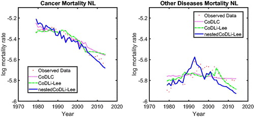
The nestedCoDLi-Lee model incorporates international coherence and intercause coherence. In the long run, the international coherence drives out the short-term shocks in one country and presents a better-behaved cause-specific mortality profile. More important, the inter-cause coherence between cancer and vascular mortality captures the catch-up effect between these two diseases to improve the forecasts for cancer mortality.

5.1.2. Out-of-Sample Performance

We compare the out-of-sample performance of all three cause-specific mortality models in terms of the root mean square error (RMSE) of the cause-specific mortality averaged over all age groups. To be concise, we present the results of the RMSEs averaged over the three countries. Figure 11 shows these averaged RMSEs for a forecast horizon from 1 to 15 years. For a forecast horizon of 1 year, we use the period 1979–2012 to estimate and forecast until 2013, for a forecast horizon of 2 years, we use the period 1979–2011 to estimate and forecast until 2013, and so on.

Figure 11. Cause-Specific Mortality RMSE Average over Three Countries.

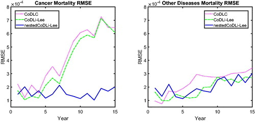
From Figure 11, we see that the out-of-sample performance of the nestedCoDLi-Lee model is better than that of the CoDLC model and that of the CoDLi-Lee model for cancer, especially for long-horizon forecasts, which is consistent with Figure 10. This is because it takes several periods for the cancer mortality changes to catch up with vascular mortality. For the cause of death with a relatively volatile historical pattern within one country (like DM), the nestedCoDLi-Lee model and CoDLi-Lee model, which take into account international coherence, could filter out the short-term volatility within one country, resulting in slightly better out-of-sample performance in the long run.

Incorporating international coherence and intercause coherence improves the forecasts of cause-specific mortality in two ways. First, because the cause-specific mortality of one country is not likely to diverge from the common trend of a coherent group in the long run, the nestedCoDLi-Lee model could capture an identifiable pattern of cause-specific mortality by summarizing the common trend from a coherent group with richer mortality data. Especially for a country with volatile historical patterns, the cause-specific mortality projections could be corrected by a similar country with more stable historical patterns. Secondly, the nestedCoDLi-Lee model, which accounts for intercause coherence, is able to capture the recent changes in cancer mortality, which might be driven by the dissemination of medical innovations from related vascular diseases. In the nestedCoDLi-Lee model, both cancer mortality and vascular mortality are expected to improve at the same speed in the long run, which leads to a faster decline in cancer mortality while forcing vascular mortality to decline slower. This catch-up of cancer mortality toward vascular mortality is captured by the nestedCoDLiLee model, contrary to the CoDLi-Lee and CoDLee-Carter models.

5.2. Part 2. All-Cause Mortality Performance

In this part, we compare the all-cause Lee-Carter model (Eq. [9]), the all-cause Li-Lee model (Eq. [5]), the CoDLC model, the CoDLi-Lee model (Eq. [10]), and the nestedCoDLi-Lee model (Eq. [15]), in terms of their in-sample fit and out-of-sample performance when considering all-cause mortality.

Table 6 summarizes the core features of the all-cause mortality models, which will be discussed in the following subsections. A model that includes cause-of-death information is one in which cause-specific mortality data are used to generate the estimations and projections for all-cause mortality. International coherence means that the model imposes that the all-cause (cause-specific) mortality of a country converges to the common trend of the countries in a coherent group. Intercause coherence means that the mortality model accounts for the intercause dynamics suggested by the two-step beta convergence test.

Table 6 All-Cause Mortality Models—Summary

	Cause of death information	International coherence	Intercause coherence
Lee-Carter	No	No	No
Li-Lee	No	Yes	No
CoDLC	Yes	No	No
CoDLi-Lee	Yes	Yes	No
nestedCoDLi-Lee	Yes	Yes	Yes

5.2.1. All-Cause Mortality Projections

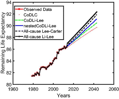
In Figure 12 we use cause-specific mortality data for The Netherlands from 1979 to 2005 to construct all-cause mortality projections until 2013 for all models, similar to Part 1 on the cause-specific mortality performance. The figure shows that the nestedCoDLi-Lee model produces the fastest-improving all-cause mortality projections, almost capturing the recent mortality changes of The Netherlands. The main driver of this is the cancer–vascular disease coherence. Incorporating this coherence helps the nestedCoDLi-Lee model to capture the catch-up effect of cancer mortality in recent years.

Figure 12. Observed, Fitted and Forecasted All-Cause Mortality, Males in The Netherlands.

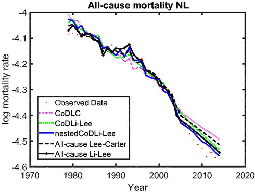
In addition, the international coherence helps both the all-cause Li-Lee model and the CoDLi-Lee model to perform better than their single-population competitors, namely, the all-cause Lee-Carter model and the CoDLC model. This is because the international coherence captures the catch-up effect and avoids divergence between different countries in a coherent group.¹⁶

5.2.2. In-Sample Fit of the All-Cause Mortality Models

We compare the fit of the LC model, the standard Li-Lee model, the CoDLC model, the CoDLi-Lee model, and the nestedCoDLi-Lee model in terms of the explanation ratios (N. Li and Lee, 2005).

Table 7 shows the explanation ratios for the different models and different countries. Among the single-population models, the all-cause LC model performs slightly better than the CoDLC model. This is because the CoDLC model needs to fit five cause-specific mortalities to construct the all-cause mortality, which includes more noise than the all-cause LC model, which directly applies to the all-cause mortality. This is also the case in the multipopulation models. Comparing the all-cause Li-Lee model to the CoDLi-Lee model and the nestedCoDLi-Lee model, the all-cause Li-Lee model performs slightly better than the latter two models, which are based on the cause-specific information. Comparing the multipopulation models to the single-population models, we discover that incorporating either all-cause mortality information or cause-specific mortality information from similar countries in a coherent group helps to improve the in-sample performance of the multipopulation models. To sum up, all of the models perform similarly, with explanation ratios over 90%.

Table 7 Explanation Ratios of the Different Models, 1979–2013 Male Population

Explanation ratios	All-cause Lee-Carter model	All-cause Li-Lee model	CoDLee-Carter model	CoDLi-Lee model	nestedCoDLi-Lee model
Belgium	0.94	0.96	0.91	0.93	0.94
France	0.91	0.98	0.90	0.97	0.95
The Netherlands	0.94	0.96	0.91	0.94	0.92

5.2.3. Out-of-Sample Performance of All-Cause Mortality Models

Figure 13 presents the all-cause mortality RMSE of the forecasts, following the same method as in Figure 11.

Figure 13. All-Cause Mortality RMSE Average over Three Countries.

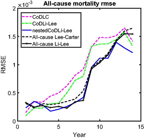
The results of the out-of-sample performance of the models in these all-cause mortality projections can be summarized as follows. First, among the cause-specific mortality models, namely, the CoDLC model (light dashed line), the CoDLi-Lee model (dash-dotted line), and the nestedCoDLi-Lee model (solid line), the nestedCoDLi-Lee model that incorporates both international coherence and intercause coherence has the best out-of-sample performance in all forecast horizons. Second, among the all-cause mortality models, namely, the all-cause LC model (heavy dashed curve) and the all-cause Li-Lee model (curve with black circles), the all-cause Li-Lee model that accounts for international coherence performs better in all forecast horizons. Third, comparing the “winner” of the cause-specific mortality models—that is, the nestedCoDLi-Lee model—and the “winner” of the all-cause mortality models—that is, the all-cause Li-Lee model—both have similar out-of-sample performance in the forecast horizon from 1 to 10 years. Once the forecast horizon becomes longer than 10 years, the nestedCoDLi-Lee model has a slightly better out-of-sample performance than the all-cause Li-Lee model, followed by the other models.

There are two main reasons why the nestedCoDLi-Lee model has comparable or even better out-of-sample performance than the all-cause mortality models. On the one hand, international coherence allows the nestedCoDLi-Lee model to identify a clear long-run trend of cause-specific mortality from richer mortality data of a coherent group, resulting in a lower country-average RMSE. On the other hand, the main intercause coherence—that is, cancer–vascular disease coherence—helps the nestedCoDLi-Lee model to capture the varying cancer mortality declines in recent years. In sum, the cancer-vascular disease coherence makes the cancer mortality projections of the nestedCoDLi-Lee model decline faster because the cancer–vascular disease common trend in the long run and maintains its own speed in the short run, thus capturing the catch-up effects of cancer mortality towards vascular mortality, which is observed in the data and confirmed by the two-step beta convergence test.

The rationale for using the nestedCoDLi-Lee model follows from the results of the two-step beta convergence test in the sample period from 1970 to 2005. More precisely, the model is set up to capture the catch-up effect between cancer and vascular diseases as suggested by the two-step beta convergence test in the sample. Suppose that a divergent pattern between cancer and vascular diseases had been detected by the two-step beta convergence; then we would not have employed the nestedCoDLi-Lee model in projecting the cause-specific mortality for these two (in this hypothetical case) divergent causes or in projecting all-cause mortality based on these cause-specific projections. In other words, if we were in a world in which the mortality trends for cancer and vascular diseases diverged, the two-step beta convergence test would signal that we should not apply the nestedCoDLi-Lee model in the projections.

5.2.4. Mortality Implications of All-Cause Mortality Models

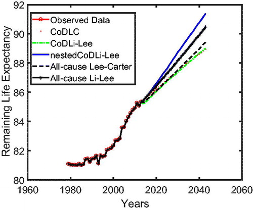
In Figure 14, we present the remaining life expectancy of a 67-year-old¹⁷ Dutch male as projected by all of the aforementioned models. The nestedCoDLi-Lee model (solid curve), which takes into account both international coherence and intercause coherence, leads to higher longevity gains than all other models in the Dutch case. More specifically, in a 30-year forecast horizon, the remaining life expectancy of a 67-year-old Dutch male is projected by the nestedCoDLi-Lee model to be approximately 1 year more than that projected by the all-cause Li-Lee model. In short, such a longevity gain is believed to come from the faster mortality declines of cancer in the mortality projections of the nestedCoDLi-Lee model, which is a consequence of cancer–vascular disease coherence.¹⁸

Figure 14. Observed and Forecasted 67-Year-Old Male Remaining Life Expectancy, Males in The Netherlands.

6. CONCLUSIONS

Using the access version of the WHO causes-of-death mortality data from 1979 to 2013 in The Netherlands, Belgium, and France, our article aims to provide all-cause mortality projections that incorporate international coherence and causes-of-death information. Based on international coherence and intercause coherence suggested by our new two-step beta convergence test, we propose a multipopulation model, referred to as nestedCoDLi-Lee, to forecast cause-specific mortality. We show that the nestedCoDLi-Lee model has an in-sample fit similar to the benchmark models used in the literature, but shows a better out-of-sample performance than the benchmark models. We attribute the merits of the nestedCoDLi-Lee model to the fact that it can prevent cause-specific turbulence within one country (for example, an influenza-like outbreak in a certain period in a specific country) and preserve well-behaved long-term forecasts by incorporating international coherence, and it can capture up-to-date intercause dynamics by allowing for intercause coherence in cause-specific mortality projections. Furthermore, we derive mortality implications in terms of all-cause mortality projections from the nestedCoDLi-Lee model and demonstrate that about additional 1-year of life expectancy could be gained by a 67-year-old Dutch male in a 30-year forecast horizon if the international coherence and intercause coherence were to continue as implied in the projections. Such longevity gains might result from more efficient intergovernmental collaborations in countries that share similar socioeconomic characteristics (international coherence) and from the dissemination of medical innovations between correlated causes of death (intercause coherence).

On the other hand, there are several limitations to the approach followed in our article. The international coherence is restricted to three countries due to limited availability of WHO access version causes of death data; the dependence structure between causes of death is highly abstracted to three types (convergence, divergence, and coherence), though there might be more possible dependence structures that are indicated by the data but are overlooked by the two-step beta convergence test. The results of the cause-specific mortality models are sensitive to the definitions of causes of death in Table 1. For future research, it would be interesting to work on constructing an approach to identify more possible dependence structures between causes of death. In addition, future research could focus on building an all-cause mortality model based on the cause-specific mortality that allows for more than one type of dependence structure between different causes of death.

ACKNOWLEDGMENTS

The authors are grateful to Richard MacMinn, Hong Li, Yang Lu, David Schrager, Jan Dob, the seminar participants at Longevity 13, and an anonymous referee for their useful comments. All errors are our responsibility.

Notes

1 Data availability restricts us to three countries at the current stage; that is, The Netherlands, Belgium, and France. Other countries—for example, the United Kingdom, United States, and Nordic countries—have a similar length of data only for some causes of death but not for all causes. Given that we would like to provide implications to all-cause mortality, we require full records for all causes-of-death mortality data. In the WHO access version database, only The Netherlands, Belgium, and France have full records of all causes-of-death mortality in the longest historical period from 1979 to 2013. In addition, the causes-of-death mortality statistics in France and The Netherlands are credited by Tabeau et al. (1999) as exceptions robust to the reclassification of diseases in the ICD.

2 We abstract from the age groups below 25 because the cause-specific data for these age groups are sparse.

3 Figure C.1 shows that mortality for DM and AMM improves at a slow and similar pace in all three countries, meaning that international coherence also holds for mortality from these minor causes. However, for UEM, we see a more volatile mortality pattern, from which we cannot draw a meaningful conclusion.

4 These rolling windows of mortality changes are defined as $d{m}_{i,t}^{s,v}=\frac{\log (m_{i,t+k}^{s,v})-\log (m_{i,t}^{s,v})}{k},$ for k = 5 and k = 10. As a default in our study, the mortality changes are represented in annual terms. Negative mortality changes indicate mortality declines, whereas positive changes indicate mortality increases.

5 For the minor causes in Figure C.2, the mortality changes are mild; that is, fluctuating around zero.

6 We also provide the related results from the Li-Lee method in the Appendix.

7 Based on the autocorrelation functions and partial autocorrelation functions (not shown in the text), we do not find evidence of autocorrelation in the residuals after controlling for a lag term.

8 The selection of the RWD for the common process K_t is the outcome of a standard Box-Jenkins procedure, where we use the Bayesian information criterion to select the best fitting model. Following Lee and Carter (1992) and N. Li and Lee (2005), we prefer a more parsimonious one over a less parsimonious one if the Bayesian information criteria are close.

9 The explanation ratio is $R_{AC}^v=1-\frac{\sum _t\sum _x[ln(m_{x,t}^v)-a_x^v-B_x{K}_t-b_x^v{k}_t^v{]}^2}{\sum _t\sum _x[ln(m_{x,t}^v)-a_x^v{]}^2}.$

10 The Li-Lee method of determining the coherent group (see Table A.1) suggests results similar to our two-step beta convergence test, except for AMM. The Li-Lee method suggests that France should be excluded from the coherent group of Belgium and The Netherlands in AMM mortality because the cause-specific mortality AMM in France is diverging away from those in Belgium and The Netherlands. On the other hand, our test shows that they are actually converging.

11 For the adult age groups and older age groups—that is, over 35 years old—we observe a cancer–vascular disease catch-up effect that starts in the mid-1990s. For the age group 25–35, cancer mortality and vascular mortality are coherent from the beginning of our sample.

12 The Li-Lee method of determining the coherent group members also supports these two coherent relationships; see Tables A.2 and A.3 in the Appendix.

13 The cause-specific Lee-Carter model consists of applying the Lee-Carter modeling approach directly to each cause-specific mortality in each country without imposing international coherence or inter-cause coherence.

14 This applies to all age groups because the two-step beta convergence test suggests no divergence for all age groups.

15 This is even more obvious for the case of Belgium (Figure C.15) and France (Figure C.16).

16 See Appendix, Figure C.17 and Figure C.18 for the similar results for Belgium and France.

17 Recently, the compulsory retirement age in The Netherlands has increased to age 67 years old.

18 See Figures C.19 and Figure C.20 for the case of Belgium and France.

19 The expectation in this appendix is taken as the conditional expectation at time t.

Appendix A. The method of determining the coherent group in No. Li and Lee (2005)

In this Appendix, we introduce the method used by N. Li and Lee (2005) to pin down the memberships of a coherent group for their model. The Li-Lee model for the cause-specific mortality for the five causes of death (s) across the three countries (v) is given as follows: (A.1) $$\begin{array}{c}ln(m_{x,t}^{s,v})={\alpha }_x^{s,v}+B_x^s{K}_t^s+b_x^{s,v}{k}_t^{s,v}+{\epsilon }_{x,t}^{s,v}.\hfill \end{array}$$(A.1)

We estimate this model using two-step SVD as described in N. Li and Lee (2005). Then, we apply the method used by their paper to determine the membership for (1) international comparison and (2) intercause comparison. The method is illustrated as follows.

A.1 International Comparison

First, the country-specific period effect $k_t^{s,v}$ for country v and cause s is fitted using an AR(1) process: (A.2) $$\begin{array}{c}{k}_t^{s,v}={\beta }_0^{s,v}+{\beta }_1^{s,v}{k}_{t-1}^{s,v}+u_t^{s,v}\hfill \end{array}$$(A.2)

Second, a coherent group membership of cause-specific mortality s could be granted to a country v, if ${\beta }_1^{s,v}<1.$ In other words, country v could only be included in this cause-specific coherent group if its country-specific period effect is a stationary process.

The results of this method are as follows. The estimation is based on data from 1979 to 2013.

From Table A.1, the Li-Lee method suggests that international coherence exists in cancer mortality, vascular mortality, other disease mortality, and unexplained mortality. However, for accidents and murders, France should be excluded from the coherent group that consists of The Netherlands and Belgium.

A.2 Intercause Comparison

A.2.1 Cancer-Vascular Coherence

Following similar logic as above, we apply the Li-Lee method to determine the inter-cause coherence between cancer and vascular diseases and obtain ${\beta }_1^{CM}$ and ${\beta }_1^{VM}$ for the cancer-specific period effect and the vascular-specific period effect. The results are in Table A.2.

A.2.2 Other Diseases and Accident Murder Coherence

Again following similar logic as above, we apply the Li-Lee method to determine the intercause coherence between other diseases and accident and murders and obtain ${\beta }_1^{DM}$ and ${\beta }_1^{\mathit{AMM}}$ presented in Table A.3.

Table A.1 Li-Lee Method of Determining Coherent Membership

${\beta }_1^{s,v}$
	CM	VM	DM	AMM	UEM
BE	0.33	0.12	0.84	0.87	0.83
FR	0.82	0.74	0.89	1.03	0.98
NL	0.16	0.43	0.81	0.94	0.88

Table A.2 Li-Lee Method, Cancer–Vascular Disease Coherence

${\beta }_1^s$
CM	0.97
VM	0.98

Table A.3 Li-Lee Method, Other Diseases–Accidents and Murders Coherence

${\beta }_1^s$
DM	0.91
AMM	0.88

Appendix B. Two-step beta convergence and its link to the Li-Lee model

In this Appendix, we provide relative proofs to the propositions.

According to Figure 4, different types of co-movements can be summarized as follows. Convergence means that the difference between two time series tends toward zero. Divergence in this context means that this difference tends toward infinity. Coherence means that this difference tends toward a constant. A negative β_level of the two-step beta convergence test indicates that the innovations of the time series are negatively related to the initial level, meaning that a higher initial level leads to lower mortality changes, whereas a lower initial level leads to higher mortality changes. This suggests that the difference between two time series with different initial levels is tending toward zero. By similar logic, a negative β_trend of the test reveals that the difference between the innovations of two time series tends toward zero. In other words, it means that these two time series increase or decrease at the same speed.

To sum up, in the context of multi-population mortality, a negative β_level indicates type 1 co-movements in Figure 4; that is, the difference between the mortality levels of the two countries tends toward zero. A negative β_trend suggests type 3 co-movements; that is, the difference between the mortality changes in the two countries tends toward zero.

Mathematically, the steady-state difference¹⁹ between the mortality levels for age x of country v and country $v\prime$ can be expressed as follows, with $v,v\prime \in \{NL,BE,FR\}$: (B.1) $$\begin{array}{c}\underset{T_L\to \infty }{\lim }[\mathbb{E}(\log (m_{x,t+T_L}^v))-\mathbb{E}(\log (m_{x,t+T_L}^{v\prime }))].\hfill \end{array}$$(B.1)

The steady-state difference between the mortality changes for age x of country v and country $v\prime$ can be expressed as follows: (B.2) $$\begin{array}{c}\underset{T_L\to \infty }{\lim }\left[\mathbb{E}\right(\frac{\log (m_{x,t+T_L+\Delta }^v)-\log (m_{x,t+T_L}^v)}{\Delta })-\mathbb{E}(\frac{\log (m_{x,t+T_L+\Delta }^{v\prime })-\log (m_{x,t+T_L}^{v\prime })}{\Delta }\left)\right].\hfill \end{array}$$(B.2)

Expressing these two differences in the Li-Lee model, we have the following equations. One is the difference between the mortality levels of two countries: (B.3) $$\begin{array}{cc}\hfill & \underset{T_L\to \infty }{\lim }[\mathbb{E}(\log (m_{x,t+T_L}^v))-\mathbb{E}(\log (m_{x,t+T_L}^{v\prime }))]\hfill \\ \hfill & =\underset{T_L\to \infty }{\lim }\mathbb{E}[{\alpha }_x^v+B_x{K}_{t+T_L}+b_x^v{k}_{t+T_L}^v-{\alpha }_x^{v\prime }-B_x{K}_{t+T_L}-b_x^{v\prime }{k}_{t+T_L}^{v\prime }]\hfill \\ \hfill & =\underset{T_L\to \infty }{\lim }[{\alpha }_x^v-{\alpha }_x^{v\prime }+b_x^v\mathbb{E}{k}_{t+T_L}^v-b_x^{v\prime }\mathbb{E}{k}_{t+T_L}^{v\prime }].\hfill \end{array}$$(B.3)

The other is the difference between the mortality changes in two countries: (B.4) $$\begin{array}{cc}\hfill & \underset{T_L\to \infty }{\lim }\left[\mathbb{E}\right(\frac{\log (m_{x,t+T_L+\Delta }^v)-\log (m_{x,t+T_L}^v)}{\Delta })-\mathbb{E}(\frac{\log (m_{x,t+T_L+\Delta }^{v\prime })-\log (m_{x,t+T_L}^{v\prime })}{\Delta }\left)\right]\hfill \\ \hfill & =\underset{T_L\to \infty }{\lim }[(B_x\mathbb{E}{K}_{t+T_L+\Delta }+b_x^v\mathbb{E}{k}_{t+T_L+\Delta }^v-B_x\mathbb{E}{K}_{t+T_L}-b_x^v\mathbb{E}{k}_{t+T_L}^v)\hfill \\ \hfill & -(B_x\mathbb{E}{K}_{t+T_L+\Delta }+b_x^{v\prime }\mathbb{E}{k}_{t+T_L+\Delta }^v-B_x\mathbb{E}{K}_{t+T_L}-b_x^{v\prime }\mathbb{E}{k}_{t+T_L}^{v\prime })].\hfill \end{array}$$(B.4)

The long-run behavior of the difference in the mortality levels and mortality changes is based on the two-step beta convergence test. To include a country in a coherent group, we need to ensure that there is no divergence in the difference in mortality levels and mortality changes between that country and the other group members. To make sure that the Li-Lee model captures the long-run behavior of these two differences, specific types of the country-specific period effect $k_t^v$ should be selected. We abstract from the discussion of the common period effect K_t because these two differences between countries will not be reflected in the K_t.

In a nutshell, we use the two-step beta convergence approach to determine whether to include a country in a coherent group. Next, we select a proper country-specific period effect to capture the international coherence suggested by the tests. We separate the selection procedure into two parts.

The first part is to assume that all countries share the same country-specific period effect. The second part is to assume that different countries could have different country-specific period effects. Both parts lead to a similar conclusion; that is, we require the country-specific period effect to be stationary in order to include this country in the coherent group. For the country-specific period effect, we consider three possible time series processes; that is, ARIMA(1, 0, 0) (AR(1)), ARIMA(0, 1, 0) (random walk with drift), and ARIMA(1, 1, 0). We do not consider including moving average components because all of the discussions in the main text focus on the best estimates without accounting for the error terms.

For the discussion below, the common period effects K_t follows an RWD. (B.5) $$\begin{array}{c}{K}_t=B_0+K_{t-1}+e_t\hfill \end{array}.$$(B.5)

B₀ is the drift term of the RWD process and e_t are random variables following an i.i.d. normal distribution.

Part 1: All countries follow the same process for the country-specific period effect.

Suppose $k_{t+T_L}^v$ follows an AR(1) process; that is, $k_{t+1}^v={\beta }_0^v+{\beta }_1^v{k}_t^v+u_t^v.$

Note that we impose a normalization on $k_t^v$ such that ${\beta }_0^v=0.$ Given a stationary AR(1) process (${\beta }_1^v$), the difference between mortality levels of two countries is as follows: (B.6) $$\begin{array}{c}\underset{T_L\to \infty }{\lim }\mathbb{E}(\hspace{0.17em}\text{log}\hspace{0.17em}(m_{x,t+T_L}^v))-\mathbb{E}(\hspace{0.17em}\text{log}\hspace{0.17em}(m_{x,t+T_L}^{v\prime }))={\alpha }_x^v-{\alpha }_x^{v\prime }+b_x^v\frac{{\beta }_0^v}{1-{\beta }_1^v}-b_x^{v\prime }\frac{{\beta }_0^{v\prime }}{1-{\beta }_1^{v\prime }}={\alpha }_x^v-{\alpha }_x^{v\prime }.\hfill \end{array}$$(B.6)

This difference in the mortality levels is constant; that is, ${\alpha }_x^v-{\alpha }_x^{v\prime }$ in Equation (B.6(B.6) $$\begin{array}{c}\underset{T_L\to \infty }{\lim }\mathbb{E}(\hspace{0.17em}\text{log}\hspace{0.17em}(m_{x,t+T_L}^v))-\mathbb{E}(\hspace{0.17em}\text{log}\hspace{0.17em}(m_{x,t+T_L}^{v\prime }))={\alpha }_x^v-{\alpha }_x^{v\prime }+b_x^v\frac{{\beta }_0^v}{1-{\beta }_1^v}-b_x^{v\prime }\frac{{\beta }_0^{v\prime }}{1-{\beta }_1^{v\prime }}={\alpha }_x^v-{\alpha }_x^{v\prime }.\hfill \end{array}$$(B.6) ). Next, the difference in mortality changes between two countries is as follows: (B.7) $$\begin{array}{cc}\hfill & \underset{T_L\to \infty }{\lim }\left[\mathbb{E}\right(\frac{\hspace{0.17em}\text{log}\hspace{0.17em}(m_{x,t+T_L+\Delta }^v)-\hspace{0.17em}\text{log}\hspace{0.17em}(m_{x,t+T_L}^v)}{\Delta })-\mathbb{E}(\frac{\hspace{0.17em}\text{log}\hspace{0.17em}(m_{x,t+T_L+\Delta }^{v\prime })-\hspace{0.17em}\text{log}\hspace{0.17em}(m_{x,t+T_L}^{v\prime })}{\Delta }\left)\right]\hfill \\ \hfill & =B_x{B}_0-B_x{B}_0=0.\hfill \end{array}$$(B.7)

To sum up, the Li-Lee model with AR(1) country-specific period effects has the following steady-state behavior: (1) the difference in mortality levels between two countries is constant given by ${\alpha }_x^v-{\alpha }_x^{v\prime }$ and (2) the difference in mortality changes between the two countries is zero. This country-specific period effect can be linked to the two possible two-step beta convergence outcomes: (1) ${\beta }_{\text{level}}<0$ and ${\beta }_{\text{trend}}<0$ with the special condition ${\alpha }_x^v-{\alpha }_x^{v\prime }=0:$ convergence and (2) ${\beta }_{\text{level}}=0$ and ${\beta }_{\text{trend}}<0:$ coherence.

Suppose $k_{t+T_L}^v$ follows an ARIMA(0, 1, 0) process; that is, $k_{t+1}^v={\beta }_0^v+k_t^v+u_t^v.$

The difference in the mortality levels between two countries is (B.8) $$\begin{array}{c}\underset{T_L\to \infty }{\lim }\mathbb{E}(\hspace{0.17em}\text{log}\hspace{0.17em}(m_{x,t+T_L}^v))-\mathbb{E}(\hspace{0.17em}\text{log}\hspace{0.17em}(m_{x,t+T_L}^{v\prime })){=}_{(b_x^v{\beta }_0^v\ne b_x^{v\prime }{\beta }_0^{v\prime })}\pm \infty \hfill \\ {=}_{(b_x^v{\beta }_0^v=b_x^{v\prime }{\beta }_0^{v\prime })}{\alpha }_x^v-{\alpha }_x^{v\prime }+b_x^v{k}_t^v-b_x^{v\prime }{k}_t^{v\prime }.\hfill \end{array}$$(B.8)

The differences between the mortality levels of two countries will become positive infinite or negative infinite under the condition that $(b_x^v{\beta }_0^v\ne b_x^{v\prime }{\beta }_0^{v\prime });$ that is, divergence. The differences could also be constant, as long as $(b_x^v{\beta }_0^v=b_x^{v\prime }{\beta }_0^{v\prime }).$

The difference in mortality changes between two countries is (B.9) $$\begin{array}{cc}\hfill & \underset{T_L\to \infty }{\lim }\left[\mathbb{E}\right(\frac{\hspace{0.17em}\text{log}\hspace{0.17em}(m_{x,t+T_L+\Delta }^v)-\hspace{0.17em}\text{log}\hspace{0.17em}(m_{x,t+T_L}^v)}{\Delta })-\mathbb{E}(\frac{\hspace{0.17em}\text{log}\hspace{0.17em}(m_{x,t+T_L+\Delta }^{v\prime })-\hspace{0.17em}\text{log}\hspace{0.17em}(m_{x,t+T_L}^{v\prime })}{\Delta }\left)\right]\hfill \\ \hfill & =b_x^v{\beta }_0^v-b_x^{v\prime }{\beta }_0^{v\prime }.\hfill \end{array}$$(B.9)

The difference in mortality changes between countries is the same if $b_x^v{\beta }_0^v=b_x^{v\prime }{\beta }_0^{v\prime }.$ If not, this difference would also stay constantly different. To sum up, this country-specific period effect links to three possible outcomes: (1) if $b_x^v{\beta }_0^v=b_x^{v\prime }{\beta }_0^{v\prime },{\beta }_{\mathit{level}}=0$ and ${\beta }_{\text{trend}}<0,$ constant difference in mortality levels and no difference in mortality changes: coherence; (2) if not, ${\beta }_{\text{level}}>0$ and ${\beta }_{\text{trend}}=0:$ divergence; (3) if ${\alpha }_x^v={\alpha }_x^{v\prime },b_x^v{k}_t^v=b_x^{v\prime }{k}_t^{v\prime }$ but $b_x^v{\beta }_0^v\ne b_x^{v\prime }{\beta }_0^{v\prime },{\beta }_{\text{level}}<0$ and ${\beta }_{\text{trend}}=0:$ convergence.

Suppose $k_t^v$ follows an ARIMA(1, 1, 0) process; that is, $k_{t+1}^v-k_t^v={\beta }_0^v+{\beta }_1^v(k_t^v-k_{t-1}^v)+u_t^v.$

Note that we impose a normalization on $k_t^v$ such that ${\beta }_0^v=0.$

For $k_t^v,$ (B.10) $$\begin{array}{c}\mathbb{E}(k_{t+T_L}^v)=\frac{1(1-{({\beta }_1^v)}^{T_L+1})}{1-{\beta }_1^v}{k}_t^v-\frac{{\beta }_1(1-{({\beta }_1^v)}^{T_L})}{1-{\beta }_1^v}{k}_{t-1}^v.\hfill \end{array}$$(B.10)

When $-1<{\beta }_1^v,{\beta }_1^{v\prime }<0,$ the limit of $k_{t+T_L}^v$ and $k_{t+T_L}^{v\prime }$ is a constant; for example $\underset{T_L\to \infty }{\lim }\mathbb{E}(k_{t+T_L}^v)=\frac{1}{1-{\beta }_1^v}{k}_t^v-\frac{{\beta }_1}{1-{\beta }_1^v}{k}_{t-1}^v.$ The differences between the mortality levels of the two countries are constants. (B.11) $$\begin{array}{cc}\underset{T_L\to \infty }{\lim }\mathbb{E}(\hspace{0.17em}\text{log}\hspace{0.17em}(m_{x,t+T_L}^v))-\mathbb{E}(\hspace{0.17em}\text{log}\hspace{0.17em}(m_{x,t+T_L}^{v\prime }))\hfill & ={\alpha }_x^v-{\alpha }_x^{v\prime }+[\frac{1}{1-{\beta }_1^v}{k}_t^v-\frac{{\beta }_1^v}{1-{\beta }_1^v}{k}_{t-1}^v]\hfill \\ \hfill & -[\frac{1}{1-{\beta }_1^{v\prime }}{k}_t^{v\prime }-\frac{{\beta }_1^v}{1-{\beta }_1^{v\prime }}{k}_{t-1}^{v\prime }].\hfill \end{array}$$(B.11)

The difference in the mortality changes between the two countries is zero when $b_x^v{\beta }_0^v=b_x^{v\prime }{\beta }_0^{v\prime }.$ If not, the mortality changes would also be different in the long run. (B.12) $$\begin{array}{cc}\hfill & \underset{T_L\to \infty }{\lim }\left[\mathbb{E}\right(\frac{\hspace{0.17em}\text{log}\hspace{0.17em}(m_{x,t+T_L+\Delta }^v)-\hspace{0.17em}\text{log}\hspace{0.17em}(m_{x,t+T_L}^v)}{\Delta })-\mathbb{E}(\frac{\hspace{0.17em}\text{log}\hspace{0.17em}(m_{x,t+T_L+\Delta }^{v\prime })-\hspace{0.17em}\text{log}\hspace{0.17em}(m_{x,t+T_L}^{v\prime })}{\Delta }\left)\right]\hfill \\ \hfill & {=}_{-1<{\beta }_1^v,{\beta }_1^{v\prime }<0}{B}_x{B}_0-B_x{B}_0=0.\hfill \end{array}$$(B.12)

When ${\beta }_1^v,{\beta }_1^{v\prime }\notin (-1,1).$ (B.13) $$\begin{array}{cc}\underset{T_L\to \infty }{\lim }\mathbb{E}(\hspace{0.17em}\text{log}\hspace{0.17em}(m_{x,t+T_L}^v))-\mathbb{E}(\hspace{0.17em}\text{log}\hspace{0.17em}(m_{x,t+T_L}^{v\prime }))\hfill & =\pm \infty \hfill \end{array}$$(B.13) (B.14) $$\begin{array}{c}\underset{T_L\to \infty }{\lim }[\mathbb{E}(\frac{\hspace{0.17em}\text{log}\hspace{0.17em}(m_{x,t+T_L+\Delta }^v)-\hspace{0.17em}\text{log}\hspace{0.17em}(m_{x,t+T_L}^v)}{\Delta })-\mathbb{E}(\frac{\hspace{0.17em}\text{log}\hspace{0.17em}(m_{x,t+T_L+\Delta }^{v\prime })-\hspace{0.17em}\text{log}\hspace{0.17em}(m_{x,t+T_L}^{v\prime })}{\Delta })]=\pm \infty \hfill \end{array}$$(B.14)

In sum, this time series process of the country-specific period effect links to two possible outcomes: (1) if $-1<{\beta }_1^v,{\beta }_1^{v\prime }<0,{\beta }_{\text{level}}=0$ and ${\beta }_{\text{trend}}<0,$ constant difference in mortality levels and no difference in mortality changes: coherence; (2) if not, ${\beta }_{\text{level}}>0$ and ${\beta }_{\text{trend}}>0:$ divergence.

Part 2: All countries have different processes of the country-specific period effect.

Suppose $k_t^v$ follows an ARIMA(1, 1, 0) process and $k_t^{v\prime }$ follows an ARIMA(1, 0, 0) process.

Considering $-1<{\beta }_1^v,{\beta }_1^{v\prime }<0$ and $0<{\beta }_1^{v\prime }<1,{\beta }_1^{v\prime }<0,$ (B.15) $$\begin{array}{cc}\underset{T_L\to \infty }{\lim }\mathbb{E}(\hspace{0.17em}\text{log}\hspace{0.17em}(m_{x,t+T_L}^v))-\mathbb{E}(\hspace{0.17em}\text{log}\hspace{0.17em}(m_{x,t+T_L}^{v\prime }))\hfill & ={\alpha }_x^v-{\alpha }_x^{v\prime }+[\frac{1}{1-{\beta }_1^v}{k}_t^v-\frac{{\beta }_1^v}{1-{\beta }_1^v}{k}_{t-1}^v]-b_x^{v\prime }\frac{{\beta }_0^{v\prime }}{1-{\beta }_1^{v\prime }}\hfill \\ \hfill & {=}_{{\beta }_0^v=0}{\alpha }_x^v-{\alpha }_x^{v\prime }+[\frac{1}{1-{\beta }_1^v}{k}_t^v-\frac{{\beta }_1^v}{1-{\beta }_1^v}{k}_{t-1}^v].\hfill \end{array}$$(B.15)

Equation (B.15(B.15) $$\begin{array}{cc}\underset{T_L\to \infty }{\lim }\mathbb{E}(\hspace{0.17em}\text{log}\hspace{0.17em}(m_{x,t+T_L}^v))-\mathbb{E}(\hspace{0.17em}\text{log}\hspace{0.17em}(m_{x,t+T_L}^{v\prime }))\hfill & ={\alpha }_x^v-{\alpha }_x^{v\prime }+[\frac{1}{1-{\beta }_1^v}{k}_t^v-\frac{{\beta }_1^v}{1-{\beta }_1^v}{k}_{t-1}^v]-b_x^{v\prime }\frac{{\beta }_0^{v\prime }}{1-{\beta }_1^{v\prime }}\hfill \\ \hfill & {=}_{{\beta }_0^v=0}{\alpha }_x^v-{\alpha }_x^{v\prime }+[\frac{1}{1-{\beta }_1^v}{k}_t^v-\frac{{\beta }_1^v}{1-{\beta }_1^v}{k}_{t-1}^v].\hfill \end{array}$$(B.15) ) shows that in the long run even if one country follows an AR(1) process and the other country follows an AR(1, 1, 0), the difference between the mortality levels of the two countries is still constant. From Equation (B.7(B.7) $$\begin{array}{cc}\hfill & \underset{T_L\to \infty }{\lim }\left[\mathbb{E}\right(\frac{\hspace{0.17em}\text{log}\hspace{0.17em}(m_{x,t+T_L+\Delta }^v)-\hspace{0.17em}\text{log}\hspace{0.17em}(m_{x,t+T_L}^v)}{\Delta })-\mathbb{E}(\frac{\hspace{0.17em}\text{log}\hspace{0.17em}(m_{x,t+T_L+\Delta }^{v\prime })-\hspace{0.17em}\text{log}\hspace{0.17em}(m_{x,t+T_L}^{v\prime })}{\Delta }\left)\right]\hfill \\ \hfill & =B_x{B}_0-B_x{B}_0=0.\hfill \end{array}$$(B.7) ) and Equation (B.9(B.9) $$\begin{array}{cc}\hfill & \underset{T_L\to \infty }{\lim }\left[\mathbb{E}\right(\frac{\hspace{0.17em}\text{log}\hspace{0.17em}(m_{x,t+T_L+\Delta }^v)-\hspace{0.17em}\text{log}\hspace{0.17em}(m_{x,t+T_L}^v)}{\Delta })-\mathbb{E}(\frac{\hspace{0.17em}\text{log}\hspace{0.17em}(m_{x,t+T_L+\Delta }^{v\prime })-\hspace{0.17em}\text{log}\hspace{0.17em}(m_{x,t+T_L}^{v\prime })}{\Delta }\left)\right]\hfill \\ \hfill & =b_x^v{\beta }_0^v-b_x^{v\prime }{\beta }_0^{v\prime }.\hfill \end{array}$$(B.9) ) we also know that both country v and country $v\prime$ share the same mortality changes; that is, $B_x{B}_0.$ Given that we have a constant mortality level difference and the same mortality changes (${\beta }_{\text{level}}=0$ and ${\beta }_{\text{trend}}<0$), we can conclude that both country v and country $v\prime$ are in the coherent group, even though they do not share the same AR processes.

Suppose $k_t^v$ follows an ARIMA(0, 1, 0) process and $k_t^{v\prime }$ follows an ARIMA(1, 0, 0) process

Considering $0<{\beta }_1^{v\prime }<1$ and only imposing ${\beta }_0^{v\prime }=0,$ because in ARIMA(0, 1, 0) the drift term is set to nonzero, (B.16) $$\begin{array}{cc}\underset{T_L\to \infty }{\lim }\mathbb{E}(\hspace{0.17em}\text{log}\hspace{0.17em}(m_{x,t+T_L}^v))-\mathbb{E}(\hspace{0.17em}\text{log}\hspace{0.17em}(m_{x,t+T_L}^{v\prime }))\hfill & =\underset{T_L\to \infty }{\lim }{\alpha }_x^v-{\alpha }_x^{v\prime }+b_x^v{\beta }_0^v{T}_L-b_x^{v\prime }\frac{{\beta }_0^{v\prime }}{1-{\beta }_1^{v\prime }}=\pm \infty \hfill \end{array}.$$(B.16)

Equation (B.16(B.16) $$\begin{array}{cc}\underset{T_L\to \infty }{\lim }\mathbb{E}(\hspace{0.17em}\text{log}\hspace{0.17em}(m_{x,t+T_L}^v))-\mathbb{E}(\hspace{0.17em}\text{log}\hspace{0.17em}(m_{x,t+T_L}^{v\prime }))\hfill & =\underset{T_L\to \infty }{\lim }{\alpha }_x^v-{\alpha }_x^{v\prime }+b_x^v{\beta }_0^v{T}_L-b_x^{v\prime }\frac{{\beta }_0^{v\prime }}{1-{\beta }_1^{v\prime }}=\pm \infty \hfill \end{array}.$$(B.16) ) shows that in the long run even if one country follows an AR(1) process and the other country follows an AR(0, 1, 0), the difference between the mortality patterns of these countries is exploding. Given that we have an exploding mortality level difference and the same mortality changes (${\beta }_{\text{level}}>0$ and ${\beta }_{\text{trend}}=0$), we can conclude that both country v and country $v\prime$ are not in the same coherent group, which is similar to the cases where all country-specific period effects share the same ARIMA(0, 1, 0) process.

Appendix C. Graphs

In this Appendix, we amend additional graphs.

Figure C.1. International Comparison: DM, AMM, and UEM Mortality Rate (Level). Note: For DM and AMM, the mortality rates of Belgium, France, and The Netherlands are relatively stationary with mild changes at some periods. The figure shows that these cause-specific mortality rates across the three countries improves at a similar pace but do not converge to the same value, implying a potential international coherence. For UEM, the mortality rates are volatile in the three countries, making it hard to draw any conclusion.

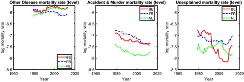
Figure C.2. International Comparison: Cancer and Vascular Mortality Changes. Note: For DM and AMM, the mortality changes of Belgium, France, and The Netherlands are converging to a similar value, which is fluctuating around zero. This is consistent with Figure C.1. The figure again implies a potential international coherence. For UEM, the results are unclear.

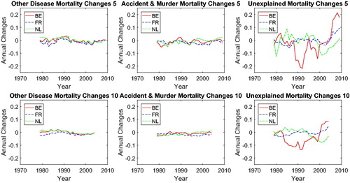
Figure C.3. International Comparison: β_slope and β_trend for DM, AMM, and UEM. Note: The left panels of the figure show that β_level of DM, AMM, and UEM is negative for all rolling window choices. The right panels show that β_trend for DM and AMM is negative for all rolling window choices, whereas that for UEM is negative for most of the rolling window choices.

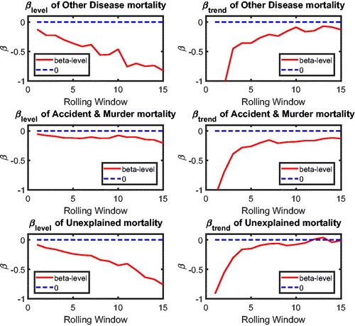
Figure C.4. International Comparison: p Value of β_slope and β_trend of DM, AMM, and UEM. Note: Combining the left panels of Figure C.3 and the left panels of this figure, we discover that the β_level for DM, AMM, and UEM is negative at the 5% significance level. With the right panels of Figure C.3 and this figure, the β_trend for DM, AMM turns out to be significantly negative for most rolling windows, whereas that for AMM turns out to be significantly negative for some rolling windows.

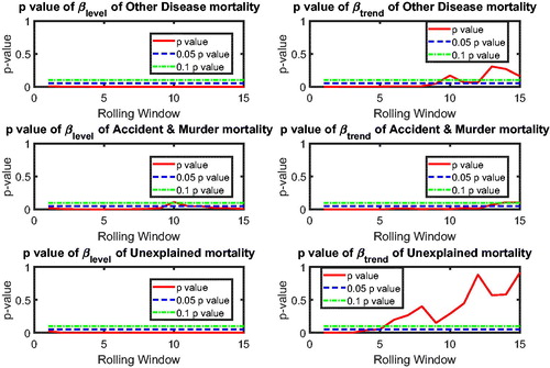
Figure C.5. Cancer-Vascular Coherence. Note: The left panels of this figure indicate that $H_0:{\beta }_{\text{level}}=0$ cannot be rejected at a significance level of 5% for all rolling window choices, meaning no sign of convergence or divergence in mortality levels of cancer (CM) and vascular mortality (VM). The right panels suggest a significant negative β_trend for most of the rolling window choices, presenting a strong evidence of cancer—vascular disease coherence.

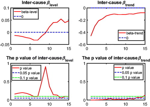
Figure C.6. No Cancer–Other Diseases Coherence. Note: The left panels of this figure indicate that $H_0:{\beta }_{\text{level}}=0$ cannot be rejected at a significance level of 5% for all rolling window choices, meaning no sign of convergence or divergence in mortality levels of cancer (CM) and other diseases (DM). The right panels suggest an insignificant β_trend at the 5% level (dotted line) for most of the rolling window choices, presenting no evidence of CM-DM coherence.

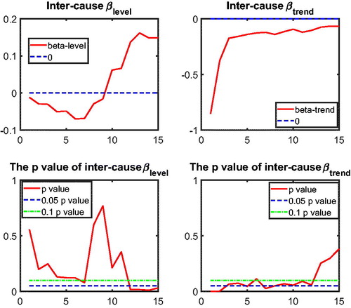
Figure C.7. No Cancer–Accidents and Murders Coherence. Note: The left panels of this figure indicate that $H_0:{\beta }_{\text{level}}=0$ cannot be rejected at a significance level of 5% for all rolling window choices, meaning no sign of convergence or divergence in mortality levels of cancer (CM) and accidents and murders (AMM). The right panels suggest an insignificant β_trend at the 5% level (dotted line) for most of the rolling window choices, presenting no evidence of CM-AMM coherence.

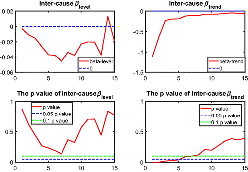
Figure C.8. No Cancer–Unexplained Coherence. Note: The left panels of this figure indicate that $H_0:{\beta }_{\text{level}}=0$ cannot be rejected at a significance level of 5% for most rolling window choices, meaning a weak sign of convergence or divergence in mortality levels of cancer (CM) and the unexplained (UEM). The right panels suggest an insignificant β_trend at 5% level (dotted line) for most of the rolling window choices, presenting no evidence of CM-UEM coherence.

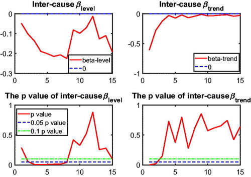
Figure C.9. No Vascular Disease–Other Disease Coherence. Note: The left panels of this figure indicate that $H_0:{\beta }_{\text{level}}=0$ cannot be rejected at a significance level of 5% for the rolling window choices with a negative β_level, meaning no sign of convergence or divergence in mortality levels of vascular (VM) and other diseases (DM). But for the rolling window choices with positive β_level, it shows a sign of significance in β_level, meaning potential divergence. The right panels suggest an insignificant β_trend at the 5% level (dotted line) for most of the rolling window choices. To sum up, it presents evidence of divergence for some rolling window choices but no evidence of VM-DM coherence.

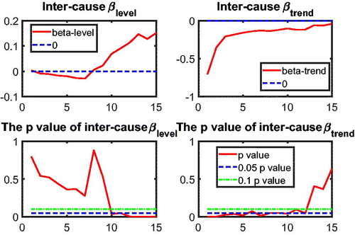
Figure C.10. No Vascular Disease–Accident and Murder Coherence. Note: The left panels of this figure indicate that $H_0:{\beta }_{\text{level}}=0$ cannot be rejected at a significance level of 5% for most rolling window choices, meaning a weak sign of convergence or divergence in mortality levels of vascular disease (VM) and accidents and murder (AMM). The right panels suggest an insignificant β_trend at the 5% level (dotted line) for most of the rolling window choices, presenting no evidence of VM-AMM coherence.

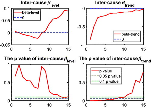
Figure C.11. No Vascular Disease–Unexplained Coherence. Note: The left panels of this figure indicate that $H_0:{\beta }_{\text{level}}=0$ cannot be rejected at a significance level of 5% for most rolling window choices, meaning a weak sign of convergence or divergence in mortality levels of vascular disease (VM) and the unexplained (UEM). The right panels suggest an insignificant β_trend at the 5% level (dotted line) for most of the rolling window choices, presenting no evidence of VM-UEM coherence.

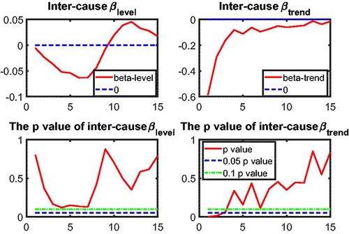
Figure C.12. Other Disease–Accident and Murder Coherence. Note: The left panels of this figure indicate that $H_0:{\beta }_{\text{level}}=0$ cannot be rejected at a significance level of 5% for most rolling window choices, meaning a weak sign of convergence or divergence in mortality levels of other diseases (DM) and accidents and murders (AMM). The right panels suggest a significant negative β_trend at the 5% level (dotted line) for most of the rolling window choices, presenting evidence of DM-AMM coherence.

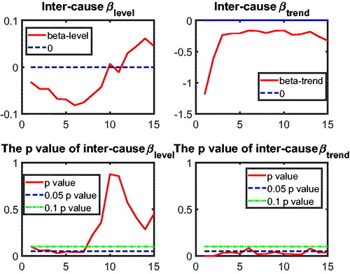
Figure C.13. No Other Disease–Unexplained Coherence. Note: The left panels of this figure indicate that $H_0:{\beta }_{\text{level}}=0$ cannot be rejected at a significance level of 5% for most rolling window choices, meaning a weak sign of convergence or divergence in mortality levels of other diseases (DM) and the unexplained (UEM). The right panels suggest an insignificant β_trend at the 5% level (dotted line) for most of the rolling window choices, presenting no evidence of DM-UEM coherence.

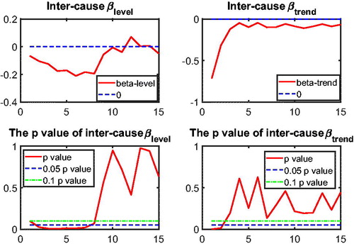
Figure C.14. Accident and Murders–Unexplained. Note: The left panels of this figure indicate that $H_0:{\beta }_{\text{level}}=0$ cannot be rejected at a significance level of 5% for most rolling window choices, meaning a weak sign of convergence or divergence in mortality levels of accidents and murders (AMM) and the unexplained (UEM). The right panels suggest an insignificant β_trend at the 5% level (dotted line) for most of the rolling window choices, presenting no evidence of AMM-UEM coherence.

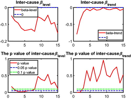
Figure C.15. Observed, Fitted, and Forecasted Cause-Specific Mortality, Males in Belgium.

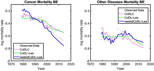
Figure C.16. Observed, Fitted, and Forecasted Cause-Specific Mortality, Males in France.

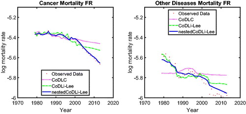
Figure C.17. Observed, Fitted, and Forecasted All-Cause Mortality, Males in Belgium. Note: For the case of Belgium, all models perform similarly, but the nestedCoDLi-Lee model produces the all-cause mortality projections that are closest to the observed data.

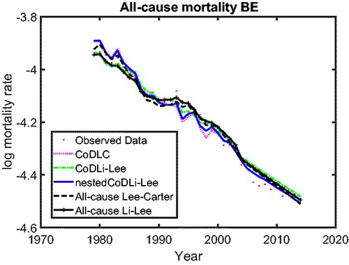
Figure C.18. Observed, Fitted, and Forecasted All-Cause Mortality, Males in France. Note: For the case of France, the models that do not account for the intercause coherence produce the closest projections to the observed data. This might result from the fact that the vascular mortality in France (blue dashed line) is improving at the slowest pace across the three countries; see Figure 3. Inter-cause coherence between cancer and vascular mortality drags the mortality changes for France slower. In addition, this outcome might result from the mortality histories that are chosen to estimate the nestedCoDLi-Lee model. Changing the estimation period might help to improve the out-of-sample performance of the nestedCoDLi-Lee model, as shown in Figure 13.

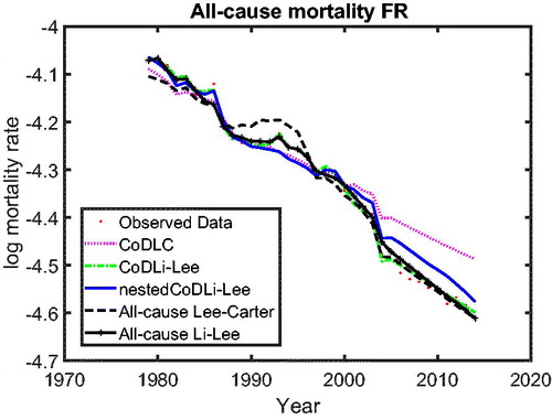
Figure C.19. Observed and Forecasted 67-Year-Old Male Remaining Life Expectancy, Males in Belgium. Note: For the case of Belgium, the remaining life expectancy of a 67-years-old male from the nestedCoDLi-Lee model is similar to that from the all-cause mortality model.

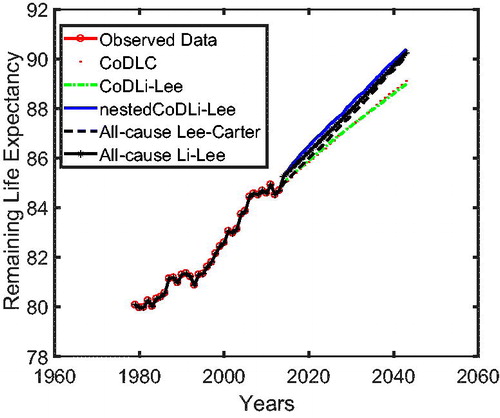
Figure C.20. Observed and Forecasted 67-Year-Old Male Remaining Life Expectancy, Males in France. Note: For the case of France, the remaining life expectancy of a 67-year-old male from the nestedCoDLi-Lee model is approximately 1 year less than that from the all-cause Li-Lee model. This is due to the international coherence that the mortality level of France could not be forever lower than that of Belgium or The Netherlands.

REFERENCES

- Adam, K., T. Jappelli, A. Menichini, M. Padula, and M. Pagano. 2002. Analyse, compare, and apply alternative indicators and monitoring methodologies to measure the evolution of capital market integration in the European Union. Centre for Studies in Economics and Finance, Department of Economics and Statistics, University of Salerno.
- Alai, D. H., S. Arnold, and M. Sherris. 2015. Modelling cause-of-death mortality and the impact of cause-elimination. Annals of Actuarial Science 9:167–86. doi:10.1017/S174849951400027X
- Arnold, S., and M. Sherris. 2013. Forecasting mortality trends allowing for cause-of-death mortality dependence. North American Actuarial Journal 17:273–82. doi:10.1080/10920277.2013.838141
- Barro, R. J. 1991. Economic growth in a cross section of countries. The Quarterly Journal of Economics, 106:407–43. doi:10.2307/2937943
- Bongaarts, J. 2014. Trends in causes of death in low-mortality countries: implications for mortality projections. Population and Development Review 40:189–212. doi:10.1111/j.1728-4457.2014.00670.x
- Booth, H., R. Hyndman, L. Tickle, and P. De Jong. 2006. Lee-carter mortality forecasting: a multi-country comparison of variants and extensions. Demographic Research 15:289–310. doi:10.4054/DemRes.2006.15.9
- Booth, H. and L. Tickle. 2008. Mortality modelling and forecasting: A review of methods. Annals of Actuarial Science 3:3–43. doi:10.1017/S1748499500000440
- Boumezoued, A., H. L. Hardy, N. El Karoui, and S. Arnold. 2018. Cause-of-death mortality: What can be learned from population dynamics? Insurance: Mathematics and Economics 78:301–15.
- Bremberg, S. G. 2017. Mortality rates in OECD countries converged during the period 1990–2010. Scandinavian Journal of Public Health 45:436–43. doi:10.1177/1403494816685529
- Cairns, A. J. G., D. Blake, and K. Dowd. 2006. A two-factor model for stochastic mortality with parameter uncertainty: Theory and calibration. Journal of Risk and Insurance 73:687–718. doi:10.1111/j.1539-6975.2006.00195.x
- Carrat, F., A. Flahault, E. Boussard, N. Farran, L. Dangoumau, and A.-J. Valleron. 1998. Surveillance of influenza-like illness in France. The example of the 1995/1996 epidemic. Journal of Epidemiology & Community Health 52:32S–38S.
- Carriere, J. F. 1994. Dependent decrement theory. Transactions of the Society of Actuaries, 46:45–74.
- Carrière, J. F. 1995. Removing cancer when it is correlated with other causes of death. Biometrical Journal 37:339–50. doi:10.1002/bimj.4710370308
- Caselli, G., J. Vallin, and M. Marsili. 2019. How useful are the causes of death when extrapolating mortality trends: An update. In Old and new perspectives on mortality forecasting, 237–259. Springer.
- d’Albis, H., L. J. Esso, and H. Pifarré i Arolas. 2012. Mortality convergence across high-income countries: An econometric approach. Working Papers of the Center of Economics of the Sorbonne 2012.76 - ISSN: 1955-611X. https://halshs.archives-ouvertes.fr/halshs-00755682.
- Dimitrova, D. S., S. Haberman, and V. K. Kaishev. 2013. Dependent competing risks: Cause elimination and its impact on survival. Insurance: Mathematics and Economics, 53:464–77. doi:10.1016/j.insmatheco.2013.07.008
- Gaille, S., and M. Sherris. 2011. Modelling mortality with common stochastic long-run trends. The Geneva Papers on Risk and Insurance Issues and Practice. 36:595–621. doi:10.1057/gpp.2011.19
- Gutterman, S., and I. T. Vanderhoof. 1998. Forecasting changes in mortality: a search for a law of causes and effects. North American Actuarial Journal 2:135–38. doi:10.1080/10920277.1998.10595759
- Hatzopoulos, P., and S. Haberman. 2013. Common mortality modeling and coherent forecasts. An empirical analysis of worldwide mortality data. Insurance: Mathematics and Economics 52:320–37. doi:10.1016/j.insmatheco.2012.12.009
- Honoré, B. E., and A. Lleras-Muney. 2006. Bounds in competing risks models and the war on cancer. Econometrica 74:1675–98. doi:10.1111/j.1468-0262.2006.00722.x
- Janssen, F. 2005. Cohort patterns in mortality trends among the elderly in seven european countries, 1950–99. International Journal of Epidemiology 34:1149–59. doi:10.1093/ije/dyi123
- Jemal, A., M. M. Center, C. DeSantis, and E. M. Ward. 2010. Global patterns of cancer incidence and mortality rates and trends. Cancer Epidemiology and Prevention Biomarkers 19:1893–1907. doi:10.1158/1055-9965.EPI-10-0437
- Kaishev, V. K., D. S. Dimitrova, and S. Haberman. 2007. Modelling the joint distribution of competing risks survival times using copula functions. Insurance: Mathematics and Economics 41:339–61. doi:10.1016/j.insmatheco.2006.11.006
- Koene, R. J., A. E. Prizment, A. Blaes, and S. H. Konety. 2016. Shared risk factors in cardiovascular disease and cancer. Circulation 133:1104–14. doi:10.1161/CIRCULATIONAHA.115.020406
- Lee, R. D., and L. R. Carter. 1992. Modeling and forecasting us mortality. Journal of the American Statistical Association 87:659–71. doi:10.2307/2290201
- Lee, R. D., and T. Miller. 2001. Evaluating the performance of the Lee-Carter method for forecasting mortality. Demography 38:537–49. doi:10.2307/3088317
- Li, H. and Y. Lu. 2019. Modeling cause-of-death mortality using hierarchical Archimedean copula. Scandinavian Actuarial Journal 2019 (3):247–272.
- Li, N., and R. Lee. 2005. Coherent mortality forecasts for a group of populations: An extension of the Lee-Carter method. Demography 42:575–94. doi:10.1353/dem.2005.0021
- Mathers, C. D., T. Boerma, and D. Ma Fat. 2009. Global and regional causes of death. British Medical Bulletin. 92 (1):7–32 doi:10.1093/bmb/ldp028
- Millossovich, P., S. Haberman, V. K. Kaishev, S. Baxter, A. Gaches, S. Gunnlaugsson, and M. Sison. 2014. Longevity basis risk a methodology for assessing basis risk. Institute and Faculty of Actuaries (IFA), Life and Longevity Markets.
- Oeppen, J. 2008. Coherent forecasting of multiple-decrement life tables: A test using japanese cause of death data. Max Planck Institute for Demographic Research Working Paper.
- Omran, A. R. 1998. The epidemiologic transition theory revisited thirty years later. World Health Statistics Quarterly 51:99–119.
- Putter, H., M. Fiocco, and R. B. Geskus. 2007. Tutorial in biostatistics: Competing risks and multi-state models. Statistics in Medicine, 26:2389–2430. doi:10.1002/sim.2712
- Renshaw, A. E., and S. Haberman. 2006. A cohort-based extension to the lee–carter model for mortality reduction factors. Insurance: Mathematics and Economics 38:556–70. doi:10.1016/j.insmatheco.2005.12.001
- Tabeau, E., P. Ekamper, C. Huisman, and A. Bosch. 1999. Improving overall mortality forecasts by analysing cause-of-death, period and cohort effects in trends. European Journal of Population/Revue Européenne de Démographie 15:153–83.
- Tabeau, E., A. van den Berg Jeths, and C. Heathcote. 2001. Forecasting mortality in developed countries: Insights from a statistical, demographic and epidemiological perspective, vol. 9. The Netherlands: Springer Science & Business Media.
- Tsiatis, A. 1975. A nonidentifiability aspect of the problem of competing risks. Proceedings of the National Academy of Sciences 72:20–22. doi:10.1073/pnas.72.1.20
- Tuljapurkar, S., N. Li, and C. Boe. 2000. A universal pattern of mortality decline in the g7 countries. Nature 405:789–92. doi:10.1038/35015561
- Vallin, J. and F. Meslé. 2004. Convergences and divergences in mortality: A new approach of health transition. Demographic Research 2:11–44. doi:10.4054/DemRes.2004.S2.2
- White, K. M. 2002. Longevity advances in high-income countries, 1955–96. Population and Development Review 28:59–76. doi:10.1111/j.1728-4457.2002.00059.x
- Wilmoth, J. R. 1995. Are mortality projections always more pessimistic when disaggregated by cause of death? Mathematical Population Studies 5:293–319. doi:10.1080/08898489509525409
- Wilmoth, J. R. 1996. Mortality projections for Japan: A comparison of four methods. In Health and mortality among elderly populations, ed. G. Caselli and A. Lopez, 266–287. Oxford: Clarendon Press.
- Wilmoth, J. R. 1998. Is the pace of japanese mortality decline converging toward international trends? Population and Development Review 24 (3):593–600. doi:10.2307/2808156
- Wilson, C. 2001. On the scale of global demographic convergence 1950–2000. Population and Development Review 27:155–71. doi:10.1111/j.1728-4457.2001.00155.x
- World Health Organisation. 2018a. International classification of diseases (ICD). http://www.who.int/classifications/icd/en/
- World Health Organisation. 2018b. WHO Mortality Database. https://www.who.int/healthinfo/mortality_data/en/
- Zheng, M., and J. P. Klein. 1995. Estimates of marginal survival for dependent competing risks based on an assumed copula. Biometrika 82:127–38. doi:10.2307/2337633