Assessment of risks to listed species from the use of atrazine in the USA: a perspective

ABSTRACT

Atrazine is a triazine herbicide used predominantly on corn, sorghum, and sugarcane in the US. Its use potentially overlaps with the ranges of listed (threatened and endangered) species. In response to registration review in the context of the Endangered Species Act, we evaluated potential direct and indirect impacts of atrazine on listed species and designated critical habitats. Atrazine has been widely studied, extensive environmental monitoring and toxicity data sets are available, and the spatial and temporal uses on major crops are well characterized. Ranges of listed species are less well-defined, resulting in overly conservative designations of “May Effect”. Preferences for habitat and food sources serve to limit exposure among many listed animal species and animals are relatively insensitive. Atrazine does not bioaccumulate, further diminishing exposures among consumers and predators. Because of incomplete exposure pathways, many species can be eliminated from consideration for direct effects. It is toxic to plants, but even sensitive plants tolerate episodic exposures, such as those occurring in flowing waters. Empirical data from long-term monitoring programs and realistic field data on off-target deposition of drift indicate that many other listed species can be removed from consideration because exposures are below conservative toxicity thresholds for direct and indirect effects. Combined with recent mitigation actions by the registrant, this review serves to refine and focus forthcoming listed species assessment efforts for atrazine.

Abbreviations: a.i. = Active ingredient (of a pesticide product). AEMP = Atrazine Ecological Monitoring Program. AIMS = Avian Incident Monitoring SystemArach. = Arachnid (spiders and mites). AUC = Area Under the Curve. BE = Biological Evaluation (of potential effects on listed species). BO = Biological Opinion (conclusion of the consultation between USEPA and the Services with respect to potential effects in listed species). CASM = Comprehensive Aquatic System Model. CDL = Crop Data LayerCN = field Curve Number. CRP = Conservation Reserve Program (lands). CTA = Conditioned Taste Avoidance. DAC = Diaminochlorotriazine (a metabolite of atrazine, also known by the acronym DACT). DER = Data Evaluation Record. EC25 = Concentration causing a specified effect in 25% of the tested organisms. EC50 = Concentration causing a specified effect in 50% of the tested organisms. EC50_RGR = Concentration causing a 50% reduction in relative growth rate. ECOS = Environmental Conservation Online System. EDD = Estimated Daily Dose. EEC = Expected Environmental Concentration. EFED = Environmental Fate and Effects Division (of the USEPA). EFSA = European Food Safety Agency. EIIS = Ecological Incident Information System. ERA = Environmental Risk Assessment. ESA = Endangered Species Act. ESU = Evolutionarily Significant UnitsFAR = Field Application RateFIFRA = Federal Insecticide, Fungicide, and Rodenticide Act. FOIA = Freedom of Information Act (request). GSD = Genus Sensitivity Distribution. HC5 = Hazardous Concentration for ≤ 5% of species. HUC = Hydrologic Unit Code. IBM = Individual-Based Model. IDS = Incident Data System. K_OC = Partition coefficient between water and organic matter in soil or sediment. K_OW = Octanol-Water partition coefficient. LC50 = Concentration lethal to 50% of the tested organisms. LC-MS-MS = Liquid Chromatograph with Tandem Mass Spectrometry. LD50 = Dose lethal to 50% of the tested organisms. LAA = Likely to Adversely Affect. LOAEC = Lowest-Observed-Adverse-Effect Concentration. LOC = Level of Concern. MA = May Affect. MATC = Maximum Acceptable Toxicant Concentration. NAS = National Academy of Sciences. NCWQR = National Center of Water Quality Research. NE = No Effect. NLAA = Not Likely to Adversely Affect. NMFS = National Marine Fisheries Service. NOAA = National Oceanic and Atmospheric Administration. NOAEC = No-Observed-Adverse-Effect Concentration. NOAEL = No-Observed-Adverse-Effect Dose-Level. OECD = Organization of Economic Cooperation and Development. PNSP = Pesticide National Synthesis Project. PQ = Plastoquinone. PRZM = Pesticide Root Zone Model. PWC = Pesticide in Water Calculator. QWoE = Quantitative Weight of Evidence. RGR = Relative growth rate (of plants). RQ = Risk Quotient. RUD = Residue Unit Doses. SAP = Science Advisory Panel (of the USEPA). SGR = Specific Growth Rate. SI = Supplemental Information. SSD = Species Sensitivity Distribution. SURLAG = Surface Runoff Lag Coefficient. SWAT = Soil & Water Assessment Tool. SWCC = Surface Water Concentration Calculator. UDL = Use Data Layer (for pesticides). USDA = United States Department of Agriculture. USEPA = United States Environmental Protection Agency. USFWS = United States Fish and Wildlife Service. USGS = United States Geological Survey. WARP = Watershed Regressions for Pesticides.

KEYWORDS:

• atrazine
• endangered species
• risk assessment
• environmental exposures
• direct effects
• indirect effects

1 Introduction

This paper was framed as a perspective to address and highlight key points about assessing risks of potential adverse effects on listed species that might result from the use of atrazine as an herbicide in the USA. This document was prepared at the request of Syngenta Crop Protection and is based on studies published in the open literature as well as those conducted by the registrant and submitted to the U.S. Environmental Protection Agency (USEPA).

1.1 Background and history

Atrazine (CAS # 1912–24-9) is a triazine herbicide that was first registered in the USA for use on corn in 1958 and has been primarily used in this crop as well as in sorghum and sugarcane since that time. In response to regulatory requirements, atrazine has been subjected to several re-registration and special reviews by the USEPA and has been the topic of 13 USEPA Science Advisory Panels, five of which were related to ecological effects. Atrazine is currently undergoing another reevaluation decision initiated in 2013 and is subject to a national endangered species assessment (referred to as a Biological Evaluation; BE) a draft of which was published in November 2020 (USEPA 2020b). Several reviews and assessments on the potential effects and risks of this chemical to aquatic organisms have been published in the scientific literature (Giddings et al. 2005; Rohr and McCoy 2010; Solomon et al. 1996, 2008). Because of its intensive properties,¹ most of the concerns regarding the potential non-target effects of atrazine have focused on residues in surface waters and risks to organisms therein. Earlier assessments (Giddings et al. 2005; Solomon et al. 1996) made use of probabilistic approaches to assess risks to aquatic organisms while later assessments (Hanson et al. 2019b; Van Der Kraak et al. 2014) utilized a Quantitative Weight of Evidence (QWoE) framework that integrated the quality of studies and relevance of any effects observed on aquatic animals in the context of potential effects at environmentally realistic exposures.

Although several of the ecological risk assessments (ERAs) for atrazine and aquatic organisms considered risks to all species through the probabilistic framework, they did not explicitly consider direct and/or indirect risks to listed (threatened and endangered) species in terrestrial and aquatic environments. However, the information on exposures and sensitivity of various species of plants and animals to atrazine is relevant to risk assessment for listed species, which, as discussed in this perspective, are generally not more sensitive to atrazine or other chemicals present in the environment. In keeping with the ESA, we have included consideration of potential indirect effects in listed species.

1.2 Risk assessment for threatened and endangered (“listed”) species

The need for a framework to address risks to listed species from use of pesticides has been highlighted (National Academy of Sciences 2013), to quote;

“The US Fish and Wildlife Service (FWS) and the National Marine Fisheries Service (NMFS)—herein called the Services—are responsible for protecting species that are listed as endangered or threatened under the Endangered Species Act (ESA) and for protecting habitats that are critical for their survival. The US Environmental Protection Agency (EPA) is responsible for registering or reregistering pesticides under the Federal Insecticide, Fungicide, and Rodenticide Act (FIFRA) and must ensure that pesticide use does not cause any unreasonable adverse effects on the environment,² which is interpreted to include listed species and their critical habitats.”

When considering potential risk resulting from exposure to pesticides, the approaches to risk assessment for listed species used by the Services are not the same as those used by the USEPA. The major difference is in the level of protection. The ESA precludes any risks that result in the loss of even a single individual of an endangered species, whereas FIFRA is a statute where risks and benefits are considered². Because of differences in legal mandate and approach, the Services, the US Department of Agriculture, and the USEPA requested the National Research Council (NRC) of the National Academy of Sciences (NAS) to examine scientific and technical issues related to determining risks posed to listed species by pesticides.

“Specifically, the NRC was asked to evaluate methods for identifying the best scientific data available; to evaluate approaches for developing modeling assumptions; to identify authoritative geospatial information that might be used in risk assessments; to review approaches for characterizing sublethal, indirect, and cumulative effects; to assess the scientific information available for estimating effects of mixtures and inert ingredients; and to consider the use of uncertainty factors to account for gaps in data.” (page 3 of National Academy of Sciences 2013).

The framework for assessing risks of pesticides to listed species as suggested by the NAS (2013) is an expansion of the traditional approach to ecological risk assessment (ERA) (USEPA 1992) and (USEPA 1998) but differs in that it includes consultation with the Services. Further guidance and interpretation of the process was outlined in an interim report from the USEPA (2015a), some of which was incorporated in a preliminary risk assessment of atrazine conducted in 2016 (USEPA 2016). More recently, the USEPA has published a newly revised method for a national-level endangered species risk assessment process for biological evaluations of pesticides (USEPA 2020e).

1.3 Previous risk assessments for listed species

Several risk assessments for atrazine and other pesticides have been conducted that include consideration of the ESA and FIFRA and risks to listed species. In 2006 and 2007, the USEPA published several risk assessments of listed species potentially exposed to atrazine. These are discussed in more detail in Section 5 and included the Barton Springs salamander which inhabits the Barton Springs complex in Texas (USEPA 2006c); five listed vertebrate species in the Chesapeake Bay watershed (the short nose sturgeon, loggerhead sea turtle, leatherback sea turtle, Kemp’s Ridley sea turtle, and green sea turtle (USEPA 2006a); the Alabama sturgeon, (USEPA 2006b); the pallid sturgeon; several species of mussels (USEPA 2007d, 2007e; 2007f); and the Topeka shiner (USEPA 2007d). In 2009, the USEPA conducted a risk assessment for atrazine in relation to the listed California red-legged frog (Rana draytonii) and Delta smelt (Hypomesus transpacificus) (2009). The risks to the Topeka shiner (Notropis topeka) from agricultural activity and habitat alteration included a mention of the use of atrazine (Panella 2012) but no detailed analysis. These assessments were conducted before guidance was published by the National Academy of Sciences (2013) and these assessments were not conducted in cooperation with the services. There are some more recent examples of risk assessments for listed species in the literature, but they were conducted for the organophosphorus insecticide malathion in the California red-legged frog, Delta smelt, as well as the California tiger salamander (Ambystoma californiense) (Clemow et al. 2018). These recent assessments more closely followed the guidance from the NAS (2013) and provide examples of the use of geospatial data, modeling of fate, and probabilistic assessment of risks to address risks of insecticides to listed species but not for an herbicide such as atrazine. Very recently, the USEPA published a draft BE of the risks of atrazine to listed aquatic and terrestrial species (USEPA 2020b)

1.4 EPA’s framework for assessing risks to listed species

The USEPA updated their draft guidance for assessment of risk to listed species in the publication “Revised Method for National Level Listed Species Biological Evaluations of Conventional Pesticides” (USEPA 2020e). This document provides a detailed description of the framework. The flow-chart for the assessment of risks to listed species from use of conventional pesticides is a stepwise process illustrated in Figure 1. The following is a brief overview of the process and some of the terminology.

Figure 1. Flow chart indicating the three steps in the EPA’s process for assessing risks to listed species (redrawn from (USEPA 2020e)). NE = no effect; MA = May Affect; LAA = Likely to Adversely Affect; NLAA = not likely to adversely affect; BE = biological evaluation; BO = biological opinion

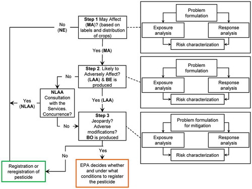
Each of the three steps in the framework (Figure 1) includes a risk characterization that has a problem formulation and analyses of exposure and response. However, the amount of data and the precision and accuracy needed increases with each step. For example, the exposure analysis in Step 1 is based on coarse information and no analysis of responses is carried out. Step 1 does not involve consultation with the Services but Steps 2 and 3 may involve informal or formal consultation with the Services.

Step 1 uses information on all designated uses (the action areas, which include the area of application and potential off-target movement of the pesticide) from the label of the pesticide and the species range or critical habitat of each listed species (see Figure 2 in USEPA 2020e). If these do not overlap or effects on single individual of the listed species are not anticipated and effects on prey, pollination, habitat, and/or dispersal are not anticipated, the species will be classified as No Effect (NE). In this case the particular registered use of the pesticide is passed through to registration. If the action area and the species range do overlap or effects on single individual of the listed species are anticipated and effects on prey, pollination, habitat, and/or dispersal are anticipated, the species will be classified as May Affect (MA). In this case, the particular registered use(s) of the pesticide advance to further assessment in Steps 2 and 3.

Figure 2. Graphical illustration of the scheme used in this assessment of risks to listed species resulting from the use of atrazine

Exposure and response information is analyzed in Steps 2 and 3. For exposures, several routes are considered, and the guidance suggests several models that can be used to estimate exposures and their consequences for Step 2 and 3 (USEPA 2020c). However, the guidance is silent on the use of measured exposures in various environmental compartments.

For Steps 1 and 2, toxicity information used for assessing potential effects on listed species considers, acute, and chronic effects on apical endpoints or responses that can be strongly linked to apical endpoints. Apical endpoints include mortality, growth, and reproduction (see Table 3 in USEPA 2020e). When sufficient toxicity data are available, the guidance suggests that probabilistic approaches such as species sensitivity distributions (SSDs) can be used. Here, the estimated 5th centile response or, if too few data are available for a SSD, that for the most sensitive species in the taxon is extrapolated to estimate adverse effects in a small proportion of the individuals. The actual slope of the exposure-effect relationship or, if the slope is unknow, a default slope of 4.5 is used.

Table 1. Best available ecotoxicology endpoints for use in ecological risk assessment of atrazine

Taxon, test endpoint, and units	Common name and species	Effect measure	Reference	USEPA MRID Number^a
Avian acute LD50 (mg/kg bw)	Bobwhite quail, Colinus virginianus	783	(Fink 1976)	00024721
Avian subacute dietary LC50 (mg/kg diet)	Mallard duck, Anas platyrhynchos	>5000	(Hill et al. 1975)	00022923
Avian chronic NOAEC (mg/kg diet)	Mallard duck, A. platyrhynchos	225	(Ciba Geigy Corp 1992)	42547101
Mammalian acute LD50 (mg/kg bw)	Rat, Rattus norvegicus	1869	(Sachsse and Bathe 1975)	00024706
Mammalian chronic NOAEL (mg/kg diet)	Rat, R. norvegicus	50	(Mainiero, et al. 1987)	40431303
Honeybee acute contact LD50 (μg/bee)	Honeybee, Apis mellifera	>97.1	(Atkins, Greywood, and Macdonald. 1975)	00036935
Honeybee acute oral LD50 (μg/bee)	Honeybee, A. mellifera	>97.1	(Atkins, Greywood, and Macdonald. 1975)	00036935
Seedling emergence EC25 (g ai/ha)	Monocot, oats, Avena sativa,	44	(Brain and Hoberg 2016)	49639102
Seedling emergence NOEC (g ai/ha)	Monocot, oats, A. sativa	28	(Brain and Hoberg 2016)	49639102
Seedling emergence EC25 (g ai/ha)	Dicot, cabbage, Brassica oleracea	11	(Brain and Hoberg 2016)	49639102
Seedling emergence NOEC (g ai/ha)	Dicot, cabbage, B. oleracea	28	(Brain and Hoberg 2016)	49639102
Vegetative vigor EC25 (g ai/ha)	Monocot, oats, A. sativa	110	(Brain and Hoberg 2016)	49639101
Vegetative vigor NOEC (g ai/ha)	Monocot, onion, Allium cepa	1.8	(Brain and Hoberg 2016)	49639101
Vegetative vigor EC25 (g ai/ha)	Dicot, cucumber, Cucumis sativa	61	(Brain and Hoberg 2016)	49639101
Vegetative vigor NOEC (g ai/ha)	Dicot, cucumber, C. sativa	5.6	(Brain and Hoberg 2016)	49639101
Freshwater fish acute LC50 (µg a.i./L)	Rainbow trout, Oncorhynchus mykiss	4500	(Beliles and Scott 1965)	00024716
Freshwater fish chronic NOEC (µg a.i./L)	Brook trout, Salvelinus fontinalis	65	(Macek et al. 1976)	00024377
Amphibian acute LC50 (µg a.i./L)	American toad, Bufo americanus late larval stage	10,700	(Howe, Gillis, and Mowbray 1998)	NA
Amphibian chronic NOEC (µg a.i./L)	Xenopus laevis	100	(Kloas et al. 2009)	47153501
Estuarine/marine fish acute LC50 (µg a.i./L)	Sheepshead minnow, Cyprinodon variegatus, adult	13,000	(Ciba Geigy Corp. 1994b)	43344901
Estuarine/marine fish chronic NOEC (µg a.i./L)	Sheepshead minnow, C. variegatus, early life stage	1100	(Syngenta 2006)	46952603
FW Invertebrate acute EC50 (µg a.i./L)	Gammarus fasciatus	720	(Macek et al. 1976)	00024377
FW Invertebrate chronic NOEC (µg a.i./L)	Daphnia magna	60	(Macek et al. 1976)	00024377
Estuarine/marine invertebrate acute EC50 (µg a.i./L)	Mysidopsis bahia	5400	(Ciba Geigy Corp. 1994a)	43344902
Estuarine/marine invertebrate acute EC50 (µg a.i./L)	Oyster, Crassostrea virginica	>17,000	(Syngenta 2005)	46648201
Green alga EC50 (µg a.i./L)	Raphidocelis subcapitata	43	(Brain et al. 2012a)	48936715
Diatom EC50 (µg a.i./L)	Navicula pelliculosa	>237	(Brain et al. 2012a)	48936714
Diatom EC50 (µg a.i./L)	Skeletonema costatum	55	(Brain et al. 2012a)	43074801
Blue-green alga EC50 (µg a.i./L)	Anabaena flos-aquae	56	(Brain et al. 2012a)	48936716
Vascular aquatic plant EC50 (µg a.i./L)	Lemna gibba	57	(Brain et al. 2012c)	46150901

^aMRID numbers are provided to facilitate access to the reference.

Table 2. Summary of atrazine chemical-physical properties and key environmental fate parameters used in Tier 3 PRZM-EXAMS modeling

Parameter	Value	Comment
Molecular weight (g/mol)	215.7	Calculated
Water solubility (mg/L at 22°C and pH 7)	33	Measured
Vapor pressure (Torr, at 25°C)	2.89 × 10^−7	Measured
Hydrolysis half-life (day)	Stable	Measured
Aqueous photolysis half-life (day)	335	Measured at pH 7, and under natural light
Aerobic soil metabolism half-life (day)	61	Calculated from 10 measured values per USEPA model input guidance
Organic carbon partition Coefficient (KOC) (mL/g)	171	Mean for 49 soils
Aerobic aqueous half-life (day)	201	Calculated from six measured values as per USEPA model input guidance
Aqueous sediment half-life (day)	311	Calculated from eight measured values as per USEPA model input guidance

Data abstracted from (Giddings et al. 2005).

Table 3. USEPA estimated values compared to model inputs (PWC, previously PWCC) of environmental fate parameters and chemical-physical properties for atrazine

Parameter	Estimated Value (EV) (EFED)^a	EFED modeling value^a
Aerobic soil metabolism (days)	139	417 (3 x EV)
KOC (ml/g)	36.94–155.34	75 (mean of 4 values)
Aerobic aqueous half-life (day)	155 and 39	277 (90% CB) Average = 96.5 SD = 82 t90,n-1 = 3.078 n = 2
Anaerobic aqueous half-life (day)	101, 49, and 608	588 (90% CB) Average = 252.6 SD = 82 t90,n-1 = 1.866 n = 3
Aqueous photolysis half-life (day)	168	168
Hydrolysis half-life (day)	Stable	Stable
Molecular weight (g/mol)	215.7	215.7
Water solubility @ 25°C (mg/L)	33	33
Vapor pressure (torr)	2.98 x × 10^−7	3.00 × 10^−7

^aData from (USEPA 2016)

Step 2 refines the assessment and characterizes individual listed species or critical habitats with greater precision to determine of the action area and the overlap with species range or critical habitat (see page 11 of USEPA 2020e). In Step 2, there are a number of conditions that are may result in a determination of Not Likely to Adversely Affect (NLAA) or Likely to Adversely Affect (LAA) for the particular use (label information) or usage (e.g., rate, number, methods, and timing of applications) and the process advances to Step 3. These are illustrated in (Figure 4 of USEPA 2020e). To summarize, a determination of NLAA will result if the any of the following are true:

• The exposure pathway is incomplete.

• The species is most likely extinct.

• The overlap of species range/critical habitat with the action area is <1%

• Based on conservative assumptions, <1 individual is exposed.

• Based on conservative assumptions, survival, growth, or reproduction will be impacted in <1 individual.

• When considering alternative assumptions for pesticide usage, weight of evidence suggests that survival, growth, or reproduction will be impacted in <1 individual.

• When considering alternative assumptions for species (e.g., population size, toxicity surrogacy, habitat, migration), the weight of evidence suggests that survival, growth, or reproduction will be impacted in <1 individual.

If none of these are true, the determination is LAA

Other criteria are used in cases where listed species are determined to be NLAA, but they have obligate relationships (e.g., they cannot survive and/or complete their life-cycle without the obligate species). Here, the obligate species is treated as if it was listed and more conservative thresholds are used to determine an “indirect” LAA for the listed species (see Table 3 and page 51 in USEPA 2020e).

The Academy (2013) and USEPA (2020e) provided generic guidance for assessing risks to listed species under FIFRA and the ESA, but no specific advice has been provided for assessing risks for any pesticides. Atrazine is an herbicide and has intensive properties such as volatility, adsorption, solubility, reactivity, persistence, and binding to the target site in the photosynthetic mechanism in plants that are different from most other pesticides. Since these properties are integral to interactions with biota, they are specific to atrazine and thus require special considerations when characterizing toxicity and potential for exposure in non-target organisms in general, and particularly in listed species. These properties were used to formulate and refine the suggestions for risk assessment in this perspective. With respect to Location-data for crops (Crop Data Layer; CDL) and use of pesticides (Use Data Layer; UDL) are well developed, especially for major crops in the conterminous US. However, this is not the case for Hawaii, the Territories, and Alaska. California and Arizona collect data on pesticide use by applicators but only that from California is available to the public.

Very recently, the USEPA published a draft BE of the risks of atrazine to listed aquatic and terrestrial species (USEPA 2020b). This perspective is not a critique of the BE; it is a perspective that highlights key information and data that is relevant to the risk assessment and should be considered when assessing the potential risks.

2. Overall problem formulation

In ERA, problem formulation is an initial and important stage in the process in that it narrows the focus and scope of the risk assessment to critical questions and risk hypotheses that are testable in the scientific sense (Suter et al. 2007). Thus, problem formulation sets the stage for the analysis plan and the amount and type of data needed. Several previous ERAs for atrazine (Giddings et al. 2005; Solomon et al. 1996; Van Der Kraak et al. 2014) have extensive problem formulations and these are not repeated here in detail; rather, the key points relevant to listed species are highlighted. The reader is referred to these earlier papers upon which this paper builds. Key properties of atrazine are highlighted in the following Sections.

2.1 Scope of this perspective

This perspective is directed to the potential effects of atrazine on listed species in the conterminous United States. Atrazine has never been labeled for use in Alaska and recent approved changes in label rescinded uses in Hawaii, and the U.S. territories (Puerto Rico, Guam, American Samoa, the U.S. Virgin Islands, and the North Mariana Islands). Roadside use is approved for removal from the label as have uses on Conservation Reserve Program (CRP) lands and forestry (see SI Section 1). Use on corn, sorghum, and sugarcane, some ornamental turf, and some fruit-trees has been retained. In addition, mitigation measures have been proposed to minimize spray drift and runoff (see Section 8 below). These label changes are in response to diminishing need for use in Hawaiian sugarcane, decreased use in roadsides, the CRP lands, and forestry. These changes in labeled uses will result in reduction in the number of listed species potentially exposed to atrazine.

Geographically, California was not included as part of the potential action area as the primary registrant (Syngenta) has no active registrations for atrazine in this state and does not intend to pursue registered uses in California in the future. Historically up to 60 products containing atrazine were registered in California but, excluding canceled products, only five products remain registered in Californa as of December 2020 (CDPR 2020). Federally, there are 454 atrazine products currently registered (USEPA 2020a), for which California represents ≈1% of those active registrations. Although atrazine has been classified as “Not Likely to be Carcinogenic to Humans” by the EPA (USEPA 2018) and the Joint FAO/WHO Meeting on Pesticide Residues (WHO 2011) concluded that atrazine is not likely to pose a carcinogenic risk to humans, it was listed on Proposition 65 (Safe Drinking Water and Toxic Enforcement Act of 1986) in California in July of 2016. Consequently, registrations and uses in CA are being phased-out. Evaluation of the California Pesticide Use Reporting (PUR) database (CDPR-PUR 2020) indicates that annual use of atrazine in CA was ≈9072 kg (20,000 lbs) between 2017 and 2019. This amount is <0.03% of the amount annually applied nationally. Moreover, the majority of recent uses in California (91%) were in Imperial County (CDPR-PUR 2020) and are expected to decrease as existing stocks decline. Consequently, it is anticipated that there will be no new registrations of atrazine in CA and current uses will decrease and eventually be phased out.

2.2 Physical, chemical, and biological properties

The physical, chemical, and biological properties of atrazine are well known and have been presented and discussed in detail in previous reviews and risk assessments of atrazine (Giddings et al. 2005; Solomon et al. 1996). Physical and chemical data that are key to characterizing environmental fate and exposures in various environmental compartments are discussed in more detail in Section 3.2.1 below. Some potential pathways of exposure can be excluded from consideration because of the physical and chemical properties of atrazine. Based on a K_OW of 501, atrazine would not be expected to bioaccumulate. Lack of bioaccumulation was confirmed in laboratory and field measurements in frogs (Edginton and Rouleau 2005) and in fish in the laboratory (Ciba Geigy Corp 1986) and in the field (Reindl, Falkowska, and Grajewska 2015). Previous reviews have concluded that atrazine does not biomagnify in the food chain (Giddings et al. 2005; Solomon et al. 1996). Thus, the key route of exposure is directly from the matrix, primarily water, but also from treated soils and plants growing therein, and direct contact with species in the action area during spraying or consumption of sprayed food items in an action area. Consequentially, biomagnification as a source of exposures in organisms in higher trophic levels is not relevant and was excluded from consideration. Lack of exposure through the food chain provides an argument for exclusion of listed species that are carnivores, invertivores, or fungivores and is applied in the assessment of terrestrial animals but does not exclude risk from direct exposures or consumption of food items (see Section 7.1.2).

2.3 Mechanism of action

The mechanism of action of atrazine is well understood and is shared with other triazines. Atrazine is a reversible inhibitor of photosynthesis (Trebst 2008) where it blocks photosynthetic transport of electrons by competitively displacing plastoquinone from a structurally specific-binding site on the D1 protein subunit of photosystem II, located in the thylakoid membrane of the chloroplast. These biochemical pathways are specific to plants and some photosynthetic bacteria and are not expressed in animals, making the triazines very selective toward plants. Toxic effects observed in animals exposed to very high doses of atrazine are mediated via other nonspecific mechanisms, such as baseline toxicity or narcosis (Barron et al. 1997). K_OW is well recognized as a driver of narcosis and atrazine has a K_OW of only 501 (see Section 3.2.1), which is consistent with the lack of sensitivity to atrazine observed in animals.

2.4 Recovery from effects

Recovery from the effects of atrazine in plants is an important consideration for risk assessment. As binding to the D1 protein subunit of photosystem II is reversible, plants have the potential to recover if the duration of exposures is not so long that energy reserves are depleted. The literature around this point is strong and consistent for freshwater macrophytes, algae, periphyton, and even terrestrial plants. Since exposures in the tissues of aquatic plants closely follow exposures in the water, aquatic macrophytes can recover from pulses of exposure (King et al. 2016; Laviale, Morin, and Creach 2011; Vallotton et al. 2008). Recovery effectively reduces risks of adverse effects on plants and related photosynthetic organisms in flowing waters, which is particularly important for characterizing indirect effects via provision of food and/or habitat to listed and non-listed species. Studies on duckweed have shown that recovery is relatively rapid and consistent, with plants exposed to concentrations of 5–80 µg/L for 1–4 days exhibiting full recovery within 7 days for growth-related endpoints (Brain, Hosmer, et al. 2012b). A study with three species of phytoplankton (Raphidocelis subcapitata, Anabaena flos-aquae, and Navicula pelliculosa) reported rapid reductions in the rate of quantum yield of photosystem II upon exposure to atrazine at 232, 887, and 237 μg/L (Brain et al. 2012a). Within 48 h of transfer to clean media, the growth-rate of these species returned to control levels at all concentrations tested. For periphyton, Prosser et al. (2013; 2015) examined the inhibition of photosystem II in field-derived communities to 24-h exposures to atrazine at concentrations from 10 to 320 µg/L. As with phytoplankton, recovery was rapid upon transfer to clean media, with exposed communities returning to within 10% of control levels within ≤ 24 h. These data show that, should exposure occur at a level where an effect is measurable, it is likely to be temporary, and not adverse in terms of continued growth and development following cessation of exposure. Thus, adverse effects are not expected unless exposures are above a biologically relevant concentration for a long enough duration to have an irreversible effect. Because of the evolutionary conservation of the photosynthetic mechanism in plants and most algae, these arguments apply to listed and non-listed plants.

2.5 Quality of data

As was pointed out in the guidance from the NAS (2013), data used in ERAs, whether for toxicity to listed or non-listed species or for exposures must be of the highest quality. This advice pertains to the sources of information (databases), the relevance of the data, and the quality of the studies (adequacy of the design, execution of data collection, the analyses that are used to characterize the data, and the reporting of the data). NAS also points out that the evaluation of data must be done in a consistent and transparent manner, regardless of source. Fortunately, atrazine has been subjected to a Quantitative Weight of Evidence (QWoE) analysis and, for aquatic animals and aquatic primary producers and communities. A large number of published studies as well as several studies submitted to regulatory agencies have been evaluated for quality and relevance (Giddings et al. 2018; Hanson et al. 2019b; Van Der Kraak et al. 2014). Data in these QWoE assessments include acute toxicity measured in the laboratory as well as data from field and semi-field studies that encompass longer-term measurements on apical endpoints such as growth, development, and reproduction in individual species and effects on entire communities of organisms tested in environmental enclosures (cosms).

2.6 Exposure

Accurate and precise knowledge of the use patterns, routes and amounts of exposure to the pesticide in question is essential to a robust and reliable ERA. Within a geospatial framework, this information is even more important for listed species than species with a more cosmopolitan distribution. While all ERAs consider the broader regions of use of the pesticide in question, this information must be known with higher resolution for listed species, the habitats of which are usually geographically confined because of specialization of ecological niches. This also means that the species-range of distribution of listed species must be known at the same spatial resolution as the exposures. These species ranges must also consider organisms, such as insects, that have different ecological niches at different stages of development. If there is no overlap of the range of listed species with a pesticide use pattern, the risk is essentially zero. This is the first step in EPA’s guidance (USEPA 2020e) and, because of this, was the first step addressed in characterizing exposures in this perspective and is based on all potential labeled uses of formulated products. This provides information on allowed normal and maximum rates of application, frequency of use, crop-types, and regional restrictions. These data for atrazine marketed by Syngenta are provided in SI Section 2, SI Table S1, which also reflects the approved removal of certain uses from the labels.

Characterization of exposure can be based on measured and/or modeled values and a knowledge of the drivers of movement and fate of the chemical in various environments. Duration and frequency of exposures of organisms are important in the assessment of potential effects of atrazine on listed species. Exposure to atrazine is dependent on the rate of transformation to metabolites and environmental degradates and, specific to flowing waters, on the hydrology of the system. Because atrazine is relatively soluble in water (33 mg/L) and has a small K_OW (log K_OW = 2.68), equilibrium between the body dose and matrix is rapidly achieved in aquatic animals such as frogs (Edginton and Rouleau 2005) and plants (Vallotton et al. 2008). Duration and frequency of exposure to atrazine were considered in the exposure (Section 3) and in characterizing risks to aquatic and terrestrial organisms in this perspective.

Timing of exposure is also important in that applications of atrazine in the USA are in the spring and early summer when it is applied pre- and early post-plant for weed control. As a result, presence in the environment is seasonal (Giddings et al. 2005; Solomon et al. 1996). Unlike insecticides and fungicides, it is only applied once or sometimes twice a year on row crops such as corn, sorghum, and sugar cane, which represented most of the use since the early 2000s (98.7% Table 3–2 in Giddings et al. 2005). With recently approved changes to the labels (see Section 2.1), use on corn, sorghum, and sugar cane will represent nearly 100% of future labeled uses in the USA (see SI Section 2) with ensuing effects on seasonality of exposures.

2.7 Effects

The influence of duration of exposure on responses is discussed above in relation to environmental exposures (Section 2.4). Risks from short exposures (≤96 h) that are infrequent are best assessed by comparison to acute toxicity values while longer exposures (weeks) are best assessed by comparison to chronic toxicity values. Atrazine is one of the best-studied agrochemicals and there is a wealth of acute and chronic toxicity data and these have been evaluated for quality.

In the context of the above discussion of responses to acute and chronic exposures, responses observed in toxicity tests do not necessarily carry equal weight in terms of their relevance to apical endpoints and sustainability of populations. All organisms respond to exposures to natural and anthropogenic chemicals in a predictable sequence related to exposure or dose. At small exposures, there might be no observable effects, but at somewhat larger exposures, homeostatic or adaptive biochemical and physiological processes, such as increased activity of detoxification enzymes, increases in stress hormones, or changes in behavior might be observed. While these changes might be statistically significant, they may not translate into biologically relevant changes in apical endpoints. They might be mere biomarkers of exposures and an entirely normal response to a stressor. Therefore, unless these responses can be causally and strongly linked to apical endpoints, they should either not be used or given proportionately less weight in risk assessment.

2.7.1 Indirect effects

As is pointed out in the NAS report (2013) and EPA’s guidance (USEPA 2020e), risk assessment of listed species must also consider indirect effects through alteration of physical habitat and via the food-web. These are best characterized by population modeling or in experimental systems such as aquatic and terrestrial cosms. However, because of resiliency and redundancy in herbivores and carnivores, small changes in populations or biomass of some food organisms do not necessarily translate into adverse effects at higher trophic levels and this needs to be factored into characterizing relevance of response.

2.7.2. Formulants

Formulated pesticides used in the environment usually contain one (or more) active ingredient(s) plus additional compounds (formulants or “inerts”) that do not have pesticidal activity but facilitate the application of the pesticide and/or increase efficacy by enhancing penetration into the target organisms. These formulants are regulated generically and lists of approved formulants are available (USEPA 2019b). If the non-target organisms have similar biochemistry and physiology to the target organism(s), these formulants might enhance uptake, and hence toxicity, in the non-target species. Formulated pesticides are not subjected to the same regimen of toxicity testing as active ingredients. Thus, adverse effects resulting from interactions between the active ingredient and the formulant(s) might not be identified except in the case of mammals, where the formulated product is subjected to acute toxicity testing in rats and rabbits. Formulated products are also used in testing for effects in non-target terrestrial plants. The formulants commonly used in end-use products containing atrazine include surfactants, anti-freeze agents, thickeners, antifoams, preservatives, and water. These formulants are only relevant in certain scenarios, such as direct deposition of the diluted formulated product on the non-target organism, e.g., because of spray drift. As has been pointed out (NAS 2013), formulants usually have physical properties that are different from the active ingredient(s) and would therefore have different fates in the environment and not co-occur in non-depositional scenarios. For this reason, assessment of risks is based on the active ingredient.

2.7.3 Mixtures

Organisms in the environment are often exposed to mixtures of pesticides rather than just a single chemical. These mixtures are of two kinds, those that result from direct application of two or more active ingredients in an application (spray) or where different chemicals, entering the matrix (e.g., flowing water) from different sources, form a mixture in the matrix. In the former case, the components and amounts in the mixture are known and, because these are assessed during the regulatory process, potential interactions have been considered and these can be applied in assessing risks in the action area. In the latter case, because these mixtures result from different uses of different chemicals at different times, it is not possible to easily regulate these under single-product regulations, such as FIFRA. As noted in the National Academy of Sciences report (2013), pesticides such as atrazine are sold as mixtures with other active ingredients or might be mixed in the spray tank and applied together by an applicator to save on costs. While these mixtures would result in simultaneous exposure to more than one chemical in organisms sprayed directly, the chemicals would have different physical, chemical, and biological properties, which would not change when mixed. Thus, they would likely not partition, degrade or, dissipate in the environment in the same way or at the same rate. Except for direct deposition on the non-target organism or deposition of drifted spray on soil or foliage, these substances will likely not be present as mixtures (in their original form) either contemporaneously or spatially in off-target areas. Moreover, the incidence of observed “synergy” (or greater than additive effects; GTA) is rare (Belden, Gilliom, and Lydy 2007; Belden et al. 2018; Cedergreen 2014), and the USEPA has issued draft guidance for evaluating pesticide mixtures (USEPA 2019c). A proposed framework for evaluation and incorporation into the ERA process was also described in Belden and Brain (2018) using a model-deviation ratio (MDR) approach. Generally, for pesticides, a single component typically dominates toxicity, suggesting that ERAs for formulations will not be meaningfully different than if based solely on the most toxic active ingredient (Belden et al. 2018).

2.8 Analysis plan

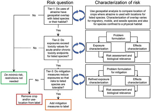
In this perspective, we have used a tiered approach based on the NAS Report (2013) and EPA’s revised guidance (USEPA 2020e) with modifications for practicality and because of the use-pattern and properties of atrazine. The tiered approach that we have used (Figure 2) is designed such that the first tier excludes situations where there is no co-occurrence of use of atrazine with listed species and is designed to minimize type-II errors. Species that are retained pass to upper tiers (if necessary) for more refined assessment. We have not consulted with the Services but have tested the risk hypotheses that would be integral to this type of Section 7 “consultation”.

2.8.1 Tier-1

This tier is a protective screening tier and is used to eliminate use patterns that have de minimis risk to listed species and approximates Step 1 in the revised guidance provided by the USEPA (2019d). There are several other criteria that USEPA suggests in its Step-1; these relate to incomplete exposure pathways (such as via bioaccumulation in the food chain as discussed above), the possibility that the listed species is extinct, and restriction of the range of the species in question to federal lands only that allows it to be excluded from further assessment.

In Tier-1 of the assessment of atrazine, geospatial data were used to test the null hypothesis that the probability of overlap between the action area for use of atrazine and the species-range for each listed species in the conterminous USA is <1% (we have used 0.95% to reduce type-2 errors). In practice, failure to reject the null hypothesis means de minimis risk of exposure for listed species in its species-range. Examples of these potential overlaps are provided in SI Section 3.

There are several additional considerations that are required for risk assessment of listed species. As noted by the USEPA (USEPA 2020e), we considered that, for some species that are migratory organisms, temporal co-occurrence would need to be addressed differently as they might not be present at all during the period of use and thus experience no exposure and no direct effects. Similarly, USEPA has recognized that dormant stages of organisms might also be protected from exposures and guidance is provided on how to incorporate this in the ERA (USEPA 2020e).

Following the suggestion of USEPA (USEPA 2020e), for terrestrial mammals, birds, reptiles, amphibians, and invertebrates, overlap was taken to mean that >0.95% of the species-range of the listed species in question overlaps temporally and spatially with the action area for use of atrazine. Given biological and environmental variability, responses to this or smaller risks of exposure would neither be observable nor testable in field studies and are essentially a de minimis risk (termed as “insignificant,” or “discountable,” by USEPA (2019d)).

Overlapping use patterns of atrazine and listed species that fail this initial screen are passed on the upper tiers for more detailed assessment. Those that pass this overlap criterion are set aside until such time as use-patterns change or the species-range of the listed species changes significantly, such as in response to climate change.

2.8.2 Tier-2

Tier-2 is used to assess the risk of potential harm to listed species where there is potential overlap of the use of atrazine and the range of listed species (Figure 2). Unlike Tier-1, there is a probability of exposure of listed species, but the amount of exposure is not known a priori and the sensitivity of the listed species in question is also not known because of the difficulty of obtaining these species for tests. The USEPA (2020e) appropriately suggested that approaches for risk assessment for various animals and plants are different. For this reason, a single method for assessing potential exposure is not provided here in the analysis plan, but rather in Section 3 below. However, there are several overarching points to be considered.

2.8.2.1 Exposures of listed species to atrazine

Although the EPA guidance (USEPA 2020e) provides suggestions modeling of exposures to pesticides, little is said about measured values and how these and modeled values can be characterized in terms of frequency of events and probability of exceedance. Knowledge of the frequency of exposures above a biologically-relevant threshold can provide useful information when characterized in relation to the time required for recovery of the affected individuals from the effect or the recovery of an affected population via propagules, resting stages, and migration (Andrus et al. 2013, 2015).

Probabilistic analysis of toxicity values is recommended as an integral component of risk assessment for listed species by the NAS report (2013) and in the guidance from USEPA (USEPA 2020e) but there is little mention of the use of probabilistic approaches for characterizing exposures. The probabilistic analysis of modeled or measured data on exposures allows it to be integrated with toxicity data to provide a joint probability of exposure and potential adverse effects in listed species such as was done in the ERA for malathion in the California red-legged frog, Delta smelt, and California tiger salamander (Clemow et al. 2018). The area under the curve (AUC) of the joint probability distribution is mathematically equivalent to the mean risk (Aldenberg, Jaworska, and Traas 2002). The AUC can be used for objective ranking of risk scenarios where data are available from multiple sites or different periods of exposure (Giddings et al. 2005) and also is useful for prioritizing areas for mitigation. The AUC has also been suggested as a criterion that can be used to classify risks, such as de minimis, intermediate, and high (Moore et al. 2014). As yet, the AUC has not been adopted as an input for regulatory decision-making.

2.8.2.2 Direct effects of atrazine on listed species

There are several important factors that need to be considered when characterizing the direct toxicity of atrazine to organisms in the environment. The most important of these relates to the mechanism of action in target organisms (usually the most sensitive) and its reversibility; the other is use of measures of effect to apical endpoints or directly relatable to these.

In discussing endpoints for assessing potential effects on listed species, USEPA guidance (USEPA 2020e) suggested that, where robust data sets of toxicity for animals or plants are available, the 5th centile of a Species Sensitivity Distribution (SSD) could be used as a point of departure for extrapolation of data on LD50s or LC50s to very small levels of mortality or inhibition of growth. The use of a 5th centile species from a SSD is a reasonable worst case for a sensitive species but there are no data indicating that listed species are inherently more sensitive to a chemical than other species; in fact the opposite has been shown to be true for plants (Christl et al. 2018). Other approaches to ERA have used the surrogate 5th centile species and generated concentration- or dose-response curves based on an average slope for the curve to extrapolate to untested species (Aldenberg, Jaworska, and Traas 2002; Clemow et al. 2018; Luttik and Aldenberg 1997; Moore et al. 2014). When there are not enough data for an SSD, USEPA (USEPA 2020e) has recommended that the toxicity value for the most sensitive species be used as a criterion for assessment. If only a few species have been tested, this might introduce uncertainty and result in an ERA that is not protective enough. While it is tempting to apply a large uncertainty factor or extrapolate the dose-response or concentration-response relationship into a realm of statistical uncertainty, this ignores common knowledge that all chemicals have thresholds below which they have no effect. This also ignores the fact that, at small doses or exposures, many substances have stimulatory or “wholly beneficial” effects (as described in USEPA 2020e) through the phenomenon of hormesis (Calabrese 2010). For these reasons, extrapolation beyond the no-observed-adverse-effect concentration (NOAEC) or dose-level, NOAEL) or the Maximum Acceptable Toxicant Concentration (MATC; where this has been estimated from the geometric mean of the NOAEC and LOAEC) is inappropriate.

Based on reviews and assessments of the toxicity data for atrazine, we considered the need for toxicity values for atrazine for use in risk assessment. Table 1 lists toxicity test endpoints that were judged to be the most suitable (best available) for use in ecological risk assessment of atrazine. Because listed species are not more sensitive to atrazine than non-listed species, these are applicable to listed and non-listed species.

2.8.2.3 Indirect effects on listed species through obligate relationships

In its guidance, USEPA (USEPA 2020e) suggests several procedures for characterizing indirect effects on listed species via direct lethal or sublethal effects on prey or food species. For added conservatism, species upon which listed species have obligate dependencies are considered as if they were listed species. A well-known biological example of obligate dependency is that between the listed black-footed ferret which is nearly completely dependent (90% of diet) on availability of prairie dogs (Cynomys spp.) The criteria for obligate animal prey are set out by USEPA (USEPA 2020e). For habitat, host, or prey species, USEPA assumes that the species-range of the listed species and the obligate species overlap. The draft BE (Attachment 4.1 in USEPA 2020b) lists a large number of obligate relationships for listed species, but clear descriptions of the nature of the relationship and whether it relates to obligate prey or host at the level of the species or a taxon is not clear. In this perspective, direct and indirect effects in general are different for target and non-target organisms and between phyla and are detailed in Sections 4 to 7. In addition, the nature of the adverse outcome pathways for the obligate hosts for some listed species are not necessarily clear (see SI Section 3.6.1 for a brief discussion of the Karner Blue butterfly). Assessment of this species is further complicated by the fact that the larval and adult stages occupy different ecological niches and likely species ranges. The adults are mobile and are generalist nectar feeders. The larval stage is an obligate feeder on the wild blue lupine.

2.8.3 Tier-3

Tier-3 assessment (Figure 2) is needed when the pesticide is determined to LAA a listed species. As the only way to reduce risk is to reduce exposure, practical and feasible measures for mitigation are considered and tested, either empirically or by modeling to determine if the proposed measures can allow the chemical, in this case atrazine, to be used without unacceptable risk to listed species. Mitigation measures may already be in place and, if they are appropriate, these would be identified in Tier-2 and a Tier-3 assessment would not be needed.

Options for mitigation can be general or specific to a species or scenario of exposure. With a wide range of potential technological and regulatory options available, we have not itemized them in this perspective but, where appropriate, this is discussed in the following Sections and in the overall recommendations in Section 8 below.

3 Uses of atrazine and exposures in the environment

3.1 Introduction

Non-target organisms can be exposed directly to pesticides during application or inadvertently via spray drift, through exposure to treated soil, or water contaminated from precipitation-induced runoff from fields treated with the chemical. When chemicals are transported from the site of application to an aquatic system, the levels found in water will be a function of a series of factors related to the both the environment as well as the properties of the chemical. Such factors include, but are not limited to, the rate of application, how frequently the runoff events occur, the magnitude of the runoff events, the timing of the runoff events relative to the time of application and the persistence of the chemical in soil and water, properties of the soil and adsorption to the constituents of the soil. Exposure-concentrations can be measured directly through analyzing water, soil, and sediment samples for chemical residues; however, for residues in water, these methods are plagued by questions of whether the highest concentrations were truly measured and if peak concentrations were missed as samples were not taken at the instant of peak concentrations in the water-body (USEPA 2016). Additionally, the costs of measuring concentrations can be prohibitively expensive for temporal sampling at multiple sites. However, a well-designed monitoring investigation with appropriate sampling intervals and reliable analysis backed up by a rigorous quality assurance plan to ensure accuracy of the data undoubtedly will yield the most useful information on exposure for purposes of risk assessment.

In the absence of extensive monitoring data sets, computer simulations of movement of the pesticide offsite can be used to estimate exposures in aquatic and terrestrial systems. There are a variety of models that can be used to predict potential exposure to aquatic and terrestrial organisms³ and these are discussed in the guidance (USEPA 2020e). However, these models do make several assumptions regarding use of the chemical, its persistence and fate, and environmental conditions. By design, these scenarios tend toward conservatism and will generally overestimate concentrations in water bodies and their variability over time. Monitoring data subjected to rigorous quality assurance and specific to locations of concern, with the appropriate level of resolution will be superior to model estimates and should be used in preference to modeling estimates. In these cases, modeling can be used in conjunction with monitoring data, where modeling assists in site selection and fills data gaps in the monitoring program. Such a synthesis of modeling and monitoring data can be used to characterize exposures that are more environmentally realistic and more useful for ecological risk assessment. As expanded upon below, the herbicide atrazine provides such an example of how an extensive historical national monitoring program can be used in conjunction with modeling to characterize potential exposures that might be experienced by listed species in the USA.

3.2 Problem formulation

3.2.1 Summary of the key properties that determine the fate of atrazine in the environment

Much of the behavior of atrazine in the environment is governed by its physical and chemical properties. There is an extensive literature database illustrating its properties, and these have been summarized previously (Giddings et al. 2005; USEPA 2016) and the most appropriate values are listed in Table 2. Overall, atrazine is hydrolytically stable under most environmentally relevant conditions as well as recalcitrant to most other abiotic degradation processes. Its primary fate pathways are microbially driven, through degradation of the alkyl side chains by N-dealkylation to deethylatrazine (DEA) and deisopropylatrazine (DIA) as well as oxidative dechlorination to hydroxyatrazine (HA). Subsequent degradation results in further n-delakylation of both alkyl sidechains to diaminochlorotriazine (DAC in Figure 2 but the other acronym, DACT, is also use in the literature), as well as the formation of desethylaminohydroxyatrazine (DEHA) and desisopropylhydroxyatrazine (DIHA). The structures of atrazine and its degradation products are shown in Figure 3.

Figure 3. Chemical structures of atrazine and its primary degradation products

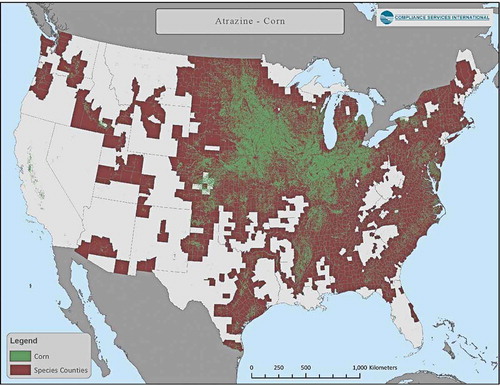
Figure 4. Distribution of corn land-use (aggregated 2010 to 2018 CDL corn data) and counties that overlap >0.95% with area of species-range for one or more listed species

Atrazine is moderately persistent under aerobic soil conditions and in aerobic aquatic conditions (Giddings et al. 2005). Atrazine is classified as moderately mobile, with K_OC values ranging from 40 to 394 based upon varying soil characteristics over a series of 49 soils (Giddings et al. 2005), and sorption is influenced by soil mineral content, pH, and organic matter content. These values, based upon laboratory measurements, make it potentially susceptible to runoff from field sites. Additionally, with low measured vapor pressure (2.89 x 10⁻⁷ torr), moderate aqueous solubility of 33 mg/L and a low Henry’s Law constant (2.6 x 10⁻⁹ atm m³ mol⁻¹), atrazine is not expected to be volatile from water or soil. Key chemical-physical properties and environmental fate parameters of atrazine are summarized in Table 2. Detailed parameter calculations for the PRZM-EXAMS model inputs were provided in Giddings et al. (2005)

Within the framework of an ecological risk assessment, choice of the appropriate environmental fate values to use will be crucial to obtaining the most representative assessment of exposure. Tables 2 and 3 summarize values for key environmental fate parameters, including aerobic soil metabolism and the soil partitioning coefficient corrected for organic matter content used in modeling exercises by the USEPA (2016) as well as in Giddings et al. (2005). Guidance from USEPA suggests using a value of 3-X the aerobic soil half-life as a conservative measure of persistence. It is interesting to note that the choices USEPA used for aerobic soil half-lives in their exposure assessment differ from those used by Giddings et al. (2005). In USEPA’s assessment, an aerobic soil metabolism average estimated half-life of 139 days was taken from three studies submitted by the registrant, and then multiplied by a 3-X factor generating a value of 417 days that was used for modeling estimates. A value of 417 days effectively renders atrazine stable to degradation by this mechanism. They further state that the value of 90th centile confidence bound half-life of 417 days is bracketed by known values in the open literature; however, the literature sources they cite are only two studies, one from 1967 (Armstrong, Chesters, and Harris 1967) and a second from 1981 (Walker and Zimdahl 1981). The expected environmental concentrations (EECs) do not significantly change when half-lives are greater than 100 days. It does not appear that shorter half-lives that are more realistic to the degradation of atrazine (30–60 days) were evaluated or that enhanced degradation of atrazine (with an average half-lives of 2.3 days) in soils from corn-growing areas in the USA have been considered (Mueller et al. 2017). Effectively, this means that USEPA (2016) significantly overestimated the persistence of atrazine. Large differences between other environmental fate parameters used in the EPA assessments and those from Giddings et al. (2005) are also observed by comparing Tables 2 and 3 with those used by USEPA. For example, Giddings et al. (2005) used the average K_OC value of 171 ml/g for 49 soils, while USEPA used a K_OC of 75 ml/g (an average of only 4 soils from a registrant-submitted study).

Giddings et al. (2005) cited half-life values from more recent studies (six papers from 1990 to 1996) ranging from 20 days to 146 days with a mean of 44 days, a value more consistent with the mean of 41 days from three other studies also cited by USEPA. The values in these studies were also representative of the reported half-lives in field soil dissipation studies submitted by Syngenta to support the registration of atrazine. At the highest tiered exposure assessment, values for these parameters were chosen based on soil characteristics specific to modeled locations (Giddings et al. 2005).

As microbial degradation is the principal route of degradation of atrazine in soil, using the proper numerical value representative of the fate of a pesticide in the field to estimate runoff is critical, especially when there are adequate amounts of monitoring data for comparison against modeled data. Where extensive monitoring data exist, it makes most sense to use actual half-lives to calibrate against modeling estimates, and the most representative degradation rates for the chemical of interest should be used in these model estimates.

3.2.2 Summary of the use of atrazine in relation to ranges of listed species

Use of atrazine has been summarized in Giddings et al. (2005), and most recently by USEPA (2016). Almost 100% of uses occur in the upper Midwest on field corn and sweet corn as well as sorghum and sugarcane, turf, and macadamia and guava in Florida. Crop distribution maps for corn, sorghum and sugarcane in relation to counties with overlap of listed species-ranges are presented in Figure 4 through Figure 6. Assessments for minor uses can easily be carried out; appropriate models are available, although species ranges would need to be defined with greater resolution.

The labeled uses of atrazine are provided in SI Section 2, SI Table S1, which reflects the approved off-labeling (SI Section 1). USEPA’s ecological risk assessment focused on these major crops as well as various turf uses, macadamia nuts, guava, roadside applications, CRP lands, and conifer use patterns. The timing of these applications is not year-round, but typically from the mid-spring to early summer for the heaviest use patterns. However, there are some uses for fallow weed control for corn, sorghum, and wheat.

There are small acreages in Florida where guava and macadamia are grown. According to the US Department of Agriculture (USDA), in 2017, total area in Florida planted with guava was 282 ha (678 A) and for macadamia nuts was 44 ha (109 A) (USDA 2019). The maximum use rate of atrazine in these tree crops is a total of 8.9 kg/ha (8 lb./A) per year for a maximum total in the two crops of 2856 kg (6296 lb.) if all crop areas were treated. Use of atrazine on macadamia and guava is not representative of typical atrazine uses across the conterminous States; it represents 0.009% of the use on corn. Assessing risks to listed species from these small uses would require more details of locations and species-ranges that are not available at this time.

Depending upon crop and formulation, atrazine can be applied by a variety of methods including aerial application, ground-boom sprayer, and tractor-drawn spreaders. When evaluating usage of atrazine, one should focus on data collected after 2003. Label usage rates were considerably higher prior to 1996. These were revised in 1996 and again in 2003. Thus, usage and monitoring data collected after this time are most representative of contemporary and future uses and hence exposures.

A caveat to the maps used in the geospatial analysis is that, for the purposes of risk assessment, these distributions only represent a snapshot in time, and specific conclusions should not be drawn solely from them. Maps of endangered species-ranges are continuously updated and cropping patterns can also change on a year-to-year basis. The guidance from USEPA (2020e) recommends the use of 5-year averages. Specific details are provided in SI Section 3.

It is important to note that the identified potential ranges at the county level for listed species are not necessarily populated by these species. In addition, counties identified as species-ranges based upon overlays of spatial data files from the US Fish and Wildlife Service (USFWS) Environmental Conservation Online System (ECOS) database with country boundary layers from the US Census Bureau can result in the assignment of the presence of a listed species to a county where it is not actually present. This error generates “false positive” results from differences in spatial processing and is described in SI Section 3.8.

An example of false-positive assignment is shown for the decurrent false aster (Boltonia decurrens, a listed terrestrial plant). A more accurate reflection of species-range is obtained by comparing the spatial overlay with current range data from the USFWS to remove counties that are artifacts of spatial data processing. Figure 7 provides a visual example of the result of this exercise that reduced an initial count of counties that included the decurrent false aster from 86 to 29.

As local crop advisors can provide specific information on treated acreage in specific locations, local ecologists could provide such information on the likely presence of protected species within habitats. While an initial highly conservative exposure assessment assumes 100% of the crop grown in a region will be treated and 100% of habitat of a protected species will contain that species, probabilistic approaches identifying the likelihood of species presence in a habitat as well as the likelihood of percent treatment of crops within an area will yield the most useful information for assessing exposure.

Likewise, all areas where crops are grown that are labeled for atrazine use will not necessarily be treated with atrazine. In each case, there is a probability that a habitat suited to an endangered species will contain that species and a probability that a region where a crop is grown will be treated with atrazine. In the latter case, local extension agents and crop advisors could provide the most reliable information of likely percent treated area based upon local knowledge of weed pressures and application practices. In the recent BE (USEPA 2020b), the USEPA estimated that from 2013 to 2017) an annual average of 32.7 × 10⁶ kg a.i. (72 × 10⁶ lbs) of atrazine were applied to an average of 30.6 × 10⁶ ha (75 × 10⁶ A) of agricultural crops. Of this, 87% was applied to corn. Use on sorghum was estimated at ca 2.9 × 10⁶ kg a.i. (ca 6.4 × 10⁶ lbs) and sugarcane ca was 0.77 × 10⁶ kg a.i. (1.7 × 10⁶ lbs). USEPA reports that only about a third of Louisiana sugarcane is treated with atrazine while virtually 100% of sugarcane in Florida is treated (USEPA 2019e).

An example of a probabilistic approach using species distribution modeling to provide a more realistic picture of species co-occurrence with crop location is provided in SI Section 3.8. After removing false positives (as above), probabilistic distribution modeling based upon locations with suitable habitat conditions further refined the area where the plant would be likely to occur (Figures 8 and 9).

3.3 Characterization of exposure

3.3.1 Routes of exposure

Pesticides applied to crops can enter both terrestrial and aquatic ecosystems from a variety of sources. Once in these systems, the chemical may reside in any number of repositories. Organisms residing in these repositories (aquatic or terrestrial receptors) can then be exposed to the chemical as can wildlife (wildlife receptors) that feed on these organisms. These pathways for exposure are depicted in Figures 10 and 11 below for aquatic and terrestrial ecosystems.

For atrazine in aquatic systems Figure 10, the principal route of exposure would be through runoff from treated fields to surface water. Some losses could occur through erosion of field soil and redeposition in surface sediment; however, given the relatively low K_OC (Table 3) and moderate water solubility, most of the atrazine transported offsite would be expected to reside in the surface water fraction as opposed to sediment. Organisms residing in surface water would be those most likely exposed to atrazine rather than benthic dwelling organisms whose major exposure would be through sediments or sediment pore water. The principal route of exposure to wildlife would be those feeding on aquatic invertebrates or aquatic plants; however, this pathway is expected to be minor as atrazine does not bioaccumulate (Giddings et al. 2005; USEPA 2016).

In terrestrial systems, principal routes of exposure are through plants and crops in the field at the point of application, as well as in surface soil or riparian areas receiving runoff from treated fields. Atrazine is taken up mostly through the roots of plants, so most exposures of non-target organisms would be expected through consumption of plants/crops either directly sprayed with atrazine or taken up by plants in soils/wetlands receiving atrazine via runoff. This is depicted in Figure 11. Atrazine has a relatively low K_OW value (USEPA 2016) and, as mentioned above, has not been shown to bioaccumulate thus exposure of wildlife through the food chain would be very unlikely.

3.3.2 Spray drift and volatilization/redeposition

Non-target organisms can be exposed to pesticides through air via spray drift or through volatilization from the point of application and redeposition through rainfall or fog. As discussed above (Section 3.2.1), atrazine has a low vapor pressure (3.0 × 10⁻⁷ torr) and moderate aqueous solubility of 33 mg/L, resulting in a low Henry’s Law constant (2.6 × 10⁻⁹ atm m³ mol⁻¹). Thus, atrazine would not be expected to be volatile from water or the surface of soil and offsite transport via volatilization and redeposition via rainfall or fog would be minimal. While some investigations have detected atrazine in trace quantities in rainfall in regions near the highest use sites (Alonso et al. 2018; USEPA 2001), this transport pathway is expected to be insignificant relative to runoff and leaching as an exposure mechanism (USEPA 2020b).

Most attempts to characterize effects of spray drift into off-field, or edge-of-field plant communities misrepresent the true way off-field exposure occurs, and subsequently overestimate risk. In agricultural settings, non-target, off-field plant communities are not typically exposed to the same rate of herbicide, or in the same manner as are in-field target plants (weeds). Edge of field deposition results primarily from interception of spray moving horizontally downwind from the sprayed crop (Figure 12). Spray drift is initially attenuated by deposition on soil between the crop and the vegetation in the field-margin and then by deposition on any vegetation present in the field-margin. Upon reaching the marginal vegetation, maximum deposition will occur in the leading edge of the vegetation and there will be rapid attenuation of deposition further into the margin, depending on the density of the plants. Vertical objects, such as plants in the field margin, are known to be more efficient collectors of airborne droplets than horizontal surfaces such as soil (Hewitt 2001) and this attenuation will protect plants deeper into the margin.

This type of exposure is not properly mimicked when potential effects of spray drift are characterized by spraying test plots from above with fractions of the field application rate (FAR, Figure 13). In this case, the horizontal extent of non-target effects is exaggerated by the even deposition across the width of the boom.

This issue has recently been addressed in a study designed to measure real-world drift of herbicide resulting from field-scale application of atrazine in order to assess in-situ, off-field non-target plant exposure and responses (Brain et al. 2019). The study combined physical deposition collectors for residue analysis with a field-based bioassay that characterized off-field effects using vegetative vigor of sensitive standard non-target terrestrial plants (cucumber and lettuce) following down-wind drift exposure from in-field atrazine application of 2.24 kg a.i./ha (2 lb. a.i./A) occurring under worst-case drift potential conditions (bare soil and wind speeds >16 km/h (>10 mph)). Note that the primary registrant of atrazine (Syngenta) has voluntarily proposed an average windspeed cap of 16 km/h (10 mph) for ground applications (see Syngenta 2020). Figure 14 shows a diagram of the layout of the study. Deposition measured on stainless steel disks decreased logarithmically with distance downwind and deposition was below background beyond 200 ft (61 m). The lowest-observed-effect-distance (LOED) was determined to be 1.5 m (5 ft) for the most sensitive plant, cucumber, and the no-observed-effect-distance (NOED) was 4.6 m (15 ft).

These empirically derived drift values contrast with those presented in the ERA conducted by USEPA (2016): “for sensitive taxa, distances extend to between 300 and 600 ft. for the coarsest droplet spectra with a low boom release height.” Since possible occurrence of drift-related effects on off-field, non-target terrestrial plants may result in implementation of impractical in-field buffer-based mitigation strategies, use of appropriate and realistic drift risk estimates is necessary. Further, effects of potential drift on terrestrial non-target plants ultimately correlate with potential risk to invertebrates, birds, and mammals present in edge-of-field habitats. TerrPlant,⁴ EPAs screening model for estimating exposure of non-target plants via drift of spray relies on endpoints derived under the presumption of direct overhead application. The fundamental issue with this approach is that it presumes non-target plants are exposed analogous to in-field target weeds (i.e., via a direct overhead spray), which is not the case (Brain et al. 2019, 2017). The guideline assays for assessing effects of pesticides on vegetative vigor⁵ and seedling emergence⁶ studies are designed to simulate a worst-case exposure by effectively saturating the foliage from a direct overhead track-sprayer, analogous to an in-field weed exposed to the maximum rate spray application. Non-target plants are off-field, and this is not how these plants are exposed. Off-field, plants are exposed to airborne drift moving laterally away from the spray swath in a path that is determined by speed and direction of the prevailing wind and receive a fraction of the applied rate that depends on the rate of sedimentation of the droplets. This phenomenon is illustrated in Figure 12, has been characterized and quantified in multiple field studies (Brain et al. 2019, 2017; De Jong and Udo De Haes 2001; Marrs and Frost 1997; Marrs, Frost, and Plant 1991a, 1991b; Marrs et al. 1989), and is illustrated in a video available for public viewing⁷

To better evaluate predicted versus actual spray drift deposition for atrazine the standard AgDRIFT® model (version 2.1.1, USEPA 2020d) was used to generate predicted spray drift deposition using EPA default assumptions as well as refined assumptions (see SI Section 4 for details of the analysis). The AgDRIFT scenarios evaluated were based on a rate of application of 2.24 kg/ha (2 lb. a.i./A) with 2 swaths. Three scenarios were modeled:

1. Tier-I EPA Default: Assumptions include high boom (50” boom height), very fine to fine droplet size distribution (DSD), 90th centile windspeed dataset

2. Tier-I EPA Refined: Assumptions include low boom (20” boom height), fine to medium/coarse DSD, 90th centile windspeed dataset

3. Tier-I EPA Refined: Assumptions include low boom (20” boom height), fine to medium/coarse DSD, 50th centile windspeed dataset

Results of this modeling (Figure 15) confirm that the Tier-1 USEPA Default model (USEPA 2016) overestimated deposition by 20- to 70-fold when compared to the measured values also shown in the figure obtained from the field measurements from Brain et al. (2019). For example, at 100 ft (30 m) from the boom, the AgDRIFT® default value for deposition was 70 times greater than the measured value (see SI Section 4, SI Table S4–1 for other values). This overestimation markedly influenced considerations of direct effects of atrazine on plants as well as indirect effects on terrestrial invertebrates, birds, and mammals in the USEPA (2016) assessment.

3.3.3 Runoff from treated fields

Atrazine is moderately water soluble with an intermediate K_OC value (Table 3), making it susceptible to storm-induced runoff from treated fields in sheet-water flow or transported on soil particles in a runoff event. This is the primary offsite transport mechanism and pathway for exposure aquatic organisms and terrestrial non-target organisms other than those located at the point of application in the field (Figures 10 and 11, above). The amount of atrazine transported in runoff will be a function of the amount of chemical applied, elapsed time from application to the rainfall event, amount and intensity of the rainfall, slope, presence, or absence of impervious layers in the soil, and properties of the soil.

While exposure models can provide estimates of concentrations of atrazine that may be present in surface waters, ultimately the best measure of exposure is from monitoring data collected from sites that will be most susceptible to runoff. These data will be most reliable and realistic for estimating exposure when collected from well-characterized watersheds with monitoring at intervals (e.g., daily) that allow estimation of peak concentrations over the course of runoff events. In addition, samples should be collected and analyzed following strict quality assurance and quality control procedures underlain by a rigorous quality management system.

3.3.3.1 Concentrations of atrazine in surface waters

The Atrazine Ecological Monitoring Program (AEMP) was developed in 2003 to meet targeted monitoring of atrazine in the most vulnerable, small headwater streams in the most vulnerable watersheds. All sites selected for the AEMP fall within the top 20% of vulnerability estimated by Watershed Regressions for Pesticides (WARP), with the vast majority of these falling within the top 10% of Hydrologic Unit Code-12 watersheds. From 2004 to 2018, this program generated 27,739 water samples representing 312 site years from 74 watersheds (80 unique sampling sites) in 13 southern and mid-western states (USEPA 2019a). Given the extent and frequency of monitoring, it is the most robust dataset for determining loadings of atrazine to small watersheds and the resulting concentrations of atrazine in surface water within these watersheds. Given that the AEMP monitoring locations are in small headwater watersheds within locations with high atrazine usage and that have characteristics making them most vulnerable to receiving runoff, this dataset reflects daily or near-daily monitoring of surface water representing the ≥80th centile of vulnerability to runoff, so it is representative of worst-case scenarios. Reanalysis of the AEMP dataset showed that the 99th centile rolling average daily, 4-d, 21-d, and 60-d concentrations of atrazine were 53, 24, 20, and 18 µg/L, respectively. From a toxicological point of view, the 4-d rolling average concentration is most appropriate for assessing the worst-case relevance of values from acute toxicology studies, whereas the 21-d and 60-d rolling averages are more appropriate to assessing chronic toxicity studies. Data from other watersheds that are less vulnerable to runoff will have smaller rolling averages and therefore are representative of less risk.

From the perspective of the ESA, species most likely to be exposed will be those in the aquatic systems receiving runoff from treated fields. Such species could include fish (e.g., Topeka shiner), amphibians, and aquatic invertebrates as well as aquatic and wetland plants. Given the mode of action of atrazine, organisms of most concern for exposure would be aquatic plants. None of the listed aquatic plant species are located within watersheds in areas of highest atrazine use as illustrated in SI Section 3, Figure 3–9 and further discussed in detail in Section 5 of this perspective.

Figure 5. Distribution of sorghum land-use (aggregated 2010 to 2018 CDL data for sorghum) and counties that overlap >0.95% with area of species-range for one or more listed species

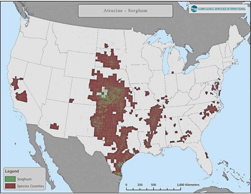
Figure 6. Distribution of sugarcane land-use (aggregated 2010 to 2018 CDL data for sugarcane) and counties that overlap >0.95% with area of species-range for one or more listed species

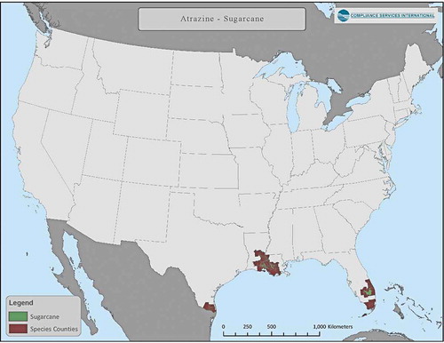
Figure 7. Distribution of counties with species-range of decurrent false aster overlapping by >0.95% with corn land-use (blue), showing counties that are false-positives (brown)

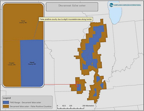
Figure 8. Results of species distribution modeling for decurrent false aster (from an unpublished report from NatureServe and Syngenta Crop Protection)

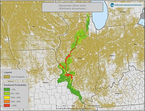
Figure 9. Results of species distribution modeling for decurrent false aster with probability >50% (red; from unpublished report from NatureServe and Syngenta Crop Protection) and the decurrent false aster range map from FWS (blue)

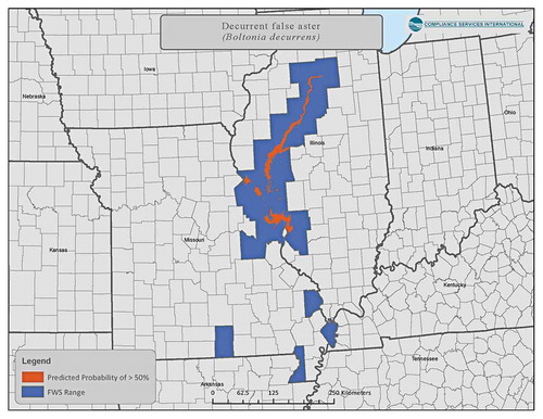
Figure 10. Pathways of exposure for aquatic and wildlife receptors in aquatic ecosystems. Arrows represent potential pathways of exposure for atrazine and the weight of the arrow indicates relative importance (see legend)

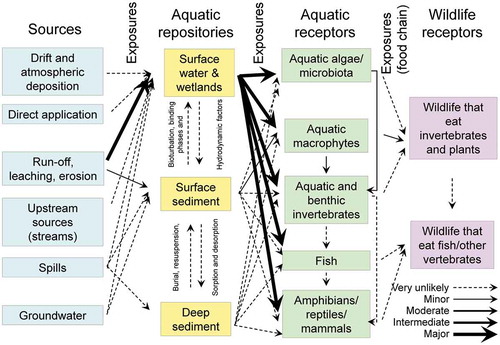
Figure 11. Pathways of exposure for terrestrial and wildlife receptors in terrestrial ecosystems. Arrows represent potential pathways of exposure for atrazine and the weight of the arrow indicates relative importance (see legend)

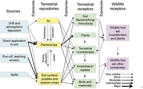
Figure 12. Diagram showing how the field margin is exposed to herbicides through spray drift from the application of herbicides to the cropped area. This scenario results in a decrease in exposure to the field margin with distance from the edge of the field (figure modified from Prosser et al. 2016)

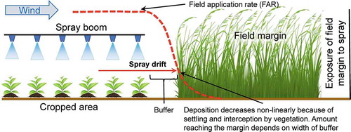
Figure 13. Field margin is exposed to herbicides through direct overspray. This scenario results in an unrealistic uniform exposure of the field margin (figure modified from Prosser et al. 2016)

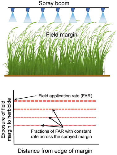
Figure 14. Diagram of the layout of the spray-drift study reported in Brain et al. (2019)

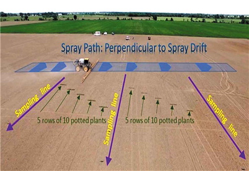
Figure 15. Comparison of measured drift deposition data from Brain et al. (2019) relative to modeled deposition using AgDRIFT® with default and refined inputs. Comparisons were made at specific distances of 12.5, 25, 50, 75, 100, 150, 200, 250, 325, and 400 ft, corresponding to the measured deposition distances defined in Brain et al. (2019). Deposition equations were used to generate the deposition curves. The vertical arrow indicates the no observed effect deposition dose for the most sensitive plant, cucumber

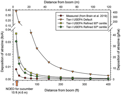
3.3.3.2 Concentrations of atrazine measured in marine waters

There is a paucity of literature reporting detections of atrazine in coastal estuarine and marine ecosystems but, given that the concentrations of atrazine found in larger watersheds are low, levels in marine systems would also be expected to be less than those in freshwater drainages in areas where atrazine is used. Hall and colleagues (1997) monitored atrazine and metabolites in the Chesapeake Bay and reported no detections above 0.22 µg/L. With a detection limit of 0.01 µg/L, the only concentration measured was in one of 20 samples taken from its main tributary, the Susquehanna River. Significantly higher concentrations were measured in smaller agriculturally influenced tributaries further up the watershed. Studies in Europe have reported concentrations of atrazine in the Mediterranean that ranged from non-detects to 0.03 µg/L with a median of 0.007 µg/L (Nödler, Licha, and Voutsa 2013) but no values above the limit of detection (0.001 µg/L) in the Baltic Sea (Nödler, Voutsa, and Licha 2014). A more recent paper using LC-MS-MS with lower limits of detection reported more frequent detections in the Yellow Sea off China (Xie et al. 2019); however, the maximum and median concentrations were small; 0.064 and 0.018 µg/L, respectively. While not directly relevant to the USA, these data from China indicate that, even in marine systems close to areas of intensive agricultural production, concentrations of atrazine in marine systems are small and that atrazine presents de minimis risk to organisms in these environments.

3.3.4 Modeling contributions of atrazine from runoff

In its Biological Evaluation for Atrazine, the USEPA (2016, 2020b) used the Pesticide Root Zone Model (PRZM5) coupled to the Variable Volume Water Model (VVWM) in the Pesticides in Water Calculator (PWC previously PWCC) as a component of the screening-level MAGTool (Magnitude of Effect Tool) to model one in fifteen-year predicted daily average expected environmental concentrations (EECs). These EECs ranged from 2.8 to 96 µg/L for Hydrologic Unit Code (HUC) 10b (Bins 6 and 7) and 81 to 5117 µg/L (HUC 11b; Bins 2 and 5).⁸ Similarly, high values were modeled previously for peak daily, 21-day, and 60-day averages (USEPA 2016). This approach used highly conservative model input parameters (e.g., entire watershed treated at the maximum application rate on the same day, unrealistically long degradation half-lives, etc.). This resulted in values inconsistent with monitoring results collected from the most highly vulnerable watersheds to runoff through the USEPA-mandated AEMP or the Heidelberg University National Center of Water Quality Research (NCWQR) program (see Figures 16 and 17). A higher tiered approach by EPA (2016) using the USGS’s WARP geospatial monitoring data-based model along with more realistic application patterns generally reduced values estimated by the SWCC between one to two orders of magnitude and estimated greater exposures for the mid-west corn belt. Unsurprisingly, this area corresponded to the major areas of use of atrazine (Syngenta 2016a).

Figure 16. Comparison of the distribution of maximum annual 60-day rolling average estimates from AEMP and NCWQR monitoring data and standard USEPA SWCC scenario exposure estimate distributions. The data from the AEMP and NCWQR are from (Syngenta 2016a)

Figure 17. Distribution of full individual/daily AEMP and NCWQR monitoring data compared to the full distribution of SWCC modeled exposure estimates from Florida sweetcorn and Midwest corn standard USEPA SWCC estimates. The data from the AEMP and NCWQR are from (Syngenta 2016a)

3.3.5 Refining monitoring data with modeling

Scenario-based modeling may use highly detailed and mechanistically constructed environmental fate models, such as the PWC, on a field scale. The exposure estimate from the PWC is essentially a high-level coarse screening only valid under hypothesized worst-case conditions (i.e., most vulnerable soil and hydrological settings, maximum product use rate, and repeated treatment of 100% of the area of the catchment, etc.). Scenario-based exposure modeling can be a useful tool to evaluate potential areas and use patterns that warrant further, higher-tiered modeling, and assessment. It should not be used to definitively describe ecological exposure and risk, especially when higher-tier targeted monitoring data are available. Higher-tier monitoring data can and should be quantitatively evaluated in an ecological risk assessment (USEPA 2014), when quality criteria are met, summarized as:

•Monitoring data should reflect areas that have a likelihood of pesticide occurrence in water, based on pesticide use as well as local runoff or leaching vulnerability

•Sampling should occur during a time frame in which pesticides are expected to be used

•Sampling frequency should be often enough to estimate exposure for endpoints of concern

•Statistical methods can be developed to address uncertainty in monitoring data and still be used quantitatively in an ecological risk assessment

•Adequate ancillary data and study design/objectives to target particular use patterns, incorporating elements of spatial and temporal patterns of exposure

When monitoring data meet criteria listed above, the data may be used in lieu of, or in addition to modeling estimates. In accordance with a quantitative evaluation of ecological risk, monitoring data can be quantitatively used as a direct measure of exposure (USEPA 2014).

An important use of monitoring data is to inform modeling to ensure that the exposure model or models are parameterized correctly and are representative of the real-world watershed characteristics and agricultural practices. One way of doing this is through model calibration where key parameters of watershed hydrology, soil properties, and use patterns are either from watershed-specific data or adjusted based on measured stream concentrations (Syngenta 2016a). In this work, a high-tier, process-based modeling approach combining the field scale Pesticide Root Zone Model (PRZM) with the watershed scale Soil & Water Assessment Tool (SWAT) model was used to predict measured stream concentrations on a daily time step. The calibrated model was then used to characterize exposure spatially and temporally to atrazine for different sizes of watersheds with a varied degree of available monitoring and environmental data. This approach offers higher certainty around less-frequent monitoring sampling designs, reducing the need for user input, and thus avoiding errors. An example of the calibrated PRZM-SWAT model for the AEMP watershed MO-2 is shown in Figures 18 and 19. This illustrates the utility of the calibrated model in characterizing flow rates and concentrations of atrazine.

Figure 18. A map of the AEMP (MO-02) Goodwater Creek watershed (drainage area = 72.5 km² (28 mile²)

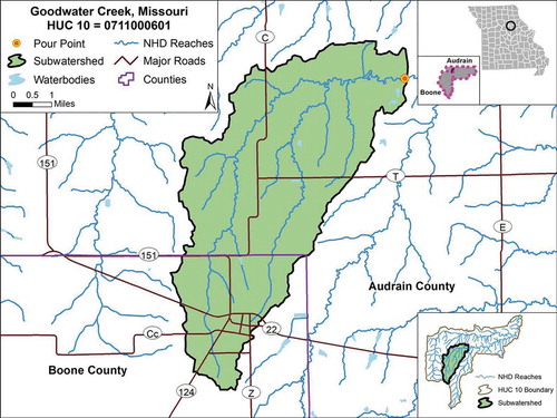
Figure 19. Measured and PRZM-SWAT model-calibrated atrazine concentrations in the stream of the AEMP (MO-02) watershed

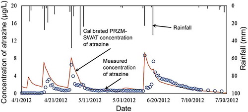
The model calibration was conducted only on the watershed hydrology parameters that determine field runoff and stream flow in the SWAT model (Syngenta 2016b). The atrazine environmental fate parameters were not calibrated, i.e., the two key parameters K_OC = 171 ml/g, and aerobic soil degradation half-life of 61 days were held constant (Table 2). Watershed hydrology calibration in SWAT was conducted using the measured stream flow at the watershed outlet between 2010 and 2014 and validated using independent flow data between 2005 and 2009 on a daily time step from the AEMP monitoring. The key hydrology parameters included SURLAG (Surface Runoff Lag Coefficient) and CN (field Curve Number). Rates of use of atrazine in watershed were estimated from the National Water-Quality Assessment Program’s (NAWQA) Pesticide National Synthesis Project (PNSP) which generates annual county-level agricultural pesticide use estimates, including atrazine, for the conterminous U.S. The county atrazine use rates were then calculated by dividing the PNSP use estimates by the total area of corn-sorghum within each county in the watershed based on the USDA Cropping Data Layer (CDL). Detailed data processing and modeling steps are described in and unpublished report (Syngenta 2016b). For the example of Figures 18 and 19, the specific atrazine use rate in 2012 was estimated at 2.121 kg/ha (1.78 lbs/A) for corn-sorghum.

Results of this modeling exercise illustrate the utility of the calibrated model in characterizing flow rates and concentrations of atrazine in small vulnerable headwater watersheds. For example, the calibrated model can be used to extend predictions for potential long-term exposure such as over 30 years required by regulatory assessments to account for temporal variability. We recognize that small headwater watersheds in AEMP may not represent all aquatic environments such as the relatively static systems (low flow dynamics) of ponds/lakes/reservoirs where listed species may use for habitats. A recent large compilation of all historical atrazine ecological water monitoring data by Syngenta (Syngenta 2017a) has more than 40,000 measured samples taken from these static aquatic systems (ponds/lakes/reservoirs) between 1996 and 2015 in the USA. The 90th centile concentration of atrazine from this comprehensive database was <6 µg/L, much lower than the 90th centile value (<12 µg/L) in the corresponding flowing systems (streams/rivers). Since all AEMP watersheds were selected by design in the highest runoff-vulnerable areas with major atrazine use, monitoring data from these streams represent the highest likely exposure among aquatic systems that are susceptible to off-target movement of atrazine. The AEMP monitoring data and its calibrated models therefore can be used as a realistic worst case for the relevant listed species assessments. We believe that these measured stream values would still be more realistic than the farm pond-based standard scenario model predictions.

Another effective way of integrating monitoring and modeling data is through a universal kriging approach (Mosquin, Aldworth, and Chen 2018; Mosquin, Whitmore, and Chen 2012) and/or SEAWAVE-QEX (Vecchia 2018) (see example in Figure 20). In these approaches, process-based models are not calibrated. Rather, model predictions can be used as covariates in a time-series regression to aid estimating concentrations for the days without sampling in a monitoring program. The advantage of this approach is that it eliminates the subjectivity that may exist in a model calibration process. An example of its use is shown in Figure 20. Note that some of the concentrations of atrazine shown in Figure 20 were measured prior to changes in rates of application in the late 1990s and that this likely explains the general decline in concentrations from 1998 onwards.

Figure 20. Observed atrazine concentrations, simulated conditional trace of daily concentrations, and estimated annual maximum daily concentrations for little buck creek near Indianapolis, Indiana (U.S. geological survey station number 03353637) for 1993–2002, from (Vecchia 2018)

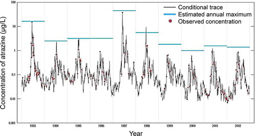
3.4 Strengths and uncertainties

The environmental fate of atrazine is well-known and is characterized with an extensive literature dataset of its partitioning and degradation in many soil types. This large data set is based upon both submitted registrant studies and published literature and yields high confidence in these parameters and allows their direct use in estimating exposure. Similarly, atrazine has the largest and highest quality water monitoring dataset for any pesticide in existence derived from watersheds located in areas with the highest intensive use. While some uncertainties exist concerning whether peak concentrations are captured, the AEMP datasets are of the highest resolution such that peaks were measured in daily sampling or can be estimated with a high degree of certainty from near-daily sampling. Thus, these monitoring values should be used instead of modeling estimates for the purposes of assessing risks.

Additionally, robust empirical field data pertaining to spray drift have been generated for atrazine, including chemical and environmental measurements along with biomonitoring of vegetative vigor, which allow direct comparisons to model simulations of drift for estimating buffers. Specific distributions of crop growing areas in geographical vicinities and percentage of treated crop are less certain. Even less certain are actual distributions of listed species within areas of atrazine use. This complicates the georeferencing of species-ranges, their overlap with crop use, and estimates of potential exposure of listed species. More accurate, refined data of actual locations of listed species will greatly reduce these uncertainties.

4 Effects of atrazine in listed aquatic plants

4.1 Problem formulation

Studies on the effects of atrazine on the few listed species of aquatic plants in the U.S. have not been published in the literature. Because of a lack of specific data for listed species, we used the large amount of information on other aquatic plants and extrapolated these findings to listed species. Atrazine could pose a risk to non-target aquatic primary producers (e.g., macrophytes, algae, periphyton), typically via reduced growth rates or, should exposures be substantial and sustained, via changes in community structure and function (Giddings et al. 2005; Moore et al. 2017; Solomon et al. 1996; Stay et al. 1989). Atrazine does not cause mortality (e.g., the complete loss of all viability with no potential for recovery) in aquatic primary producers at environmentally relevant or considerably greater concentrations under laboratory or field conditions and for realistic exposure durations (see Section 2.4).

As noted in Section 2, there is no evidence of atrazine bioaccumulating in algae or plants beyond general uptake as would be expected for an herbicide with its specific physicochemical properties. This means that concentrations in primary producers would be expected to decline rapidly upon the cessation of exposure. Experimentally, it has been shown that, upon the termination of exposure to atrazine the inhibition of photosystem II ceases with recovery (e.g., a return to control level rates of photosynthesis) observed on the order of hours to days (see Section 2.4 above). As exposures, especially in lotic systems, are typically pulsed in nature, there is a significant window for recovery to occur, should there be any impairment of growth (King et al. 2016).

Exposures to aquatic and riparian habitats, marine and freshwater, are typically driven by run-off from the site of application following significant rainfall events (see Section 3.3) as opposed to spray drift. In lotic systems, these tend to be pulsed, with a peak of exposure followed by a decline. In lentic systems, such as farm ponds with no outflow, exposures tend to be more chronic, due to the relatively long half-life of atrazine (see Section 3.2.1). Exposure concentrations in worst-case scenarios in lotic systems (i.e., those watersheds identified under the AEMP) upper 90th centiles of exposure concentrations are in the 10s of µg/L range (see Section 3.3.3.1). As the movement of atrazine into aquatic ecosystems is primarily via run-off, other material is often associated with exposure to atrazine. This includes sediments (e.g., organic matter, clay, and sand) and nutrients, which, in turn, can result in increased turbidity and eutrophication, respectively (Andrus et al. 2013, 2015; Dalton, Boutin, and Pick 2015), contributing to impaired water quality that can impact aquatic plants. In marine ecosystems, exposure to atrazine is typically in the very low (ng/L) range, and inputs are predominately via riverine inputs to nearshore environments (see Section 3.3.3.2).

4.2 Listed species at risk

Currently (as of 2019) in the conterminous USA, there are seven aquatic plants listed as endangered.⁹ In addition, there are several listed species of wetland plants, such as the decurrent false aster (Boltonia decurrens), that might be exposed to atrazine via surface waters; these are discussed in Sections 3.2.2 and 6. There are no algal species (marine or freshwater), or any other fully aquatic primary producers listed under the ESA in the conterminous USA. Listed species are the freshwater dicots Amphianthus pusillus (Little amphianthus) and Nasturtium gambelii (Gambel’s watercress); freshwater monocots Potamogeton clystocarpus (Little Aguja pondweed) and Sagittaria secundifolia (Kral’s water-plantain); the freshwater pteridophytes Isoetes melanospora (black-spored quillwort) and Isoetes tegetiformans (mat-forming quillwort); and the marine dicot Halophila johnsonii (Johnson’s seagrass). The perennial herb Nasturtium gambelii (Gambel’s watercress) is also listed but is only found in California, where Syngenta has no active registration for atrazine. Therefore, it was excluded from this assessment of risks. Locations of the remaining six species are described below.

The annual herb Amphianthus pusillus (little amphianthus) is found in fewer than 100 locations in Alabama, South Carolina, and predominantly Georgia⁹ in shallow pools on granite outcrops. There is a very low likelihood of corn production on rock outcrops; however, there is an overlap of the species-range for little amphianthus and the crop coverage that is between 1 and 2% (Figure 21 and SI Section 3, SI Table S3–3).

Figure 21. Map showing county-level distribution of the listed aquatic plant species except for Gambel’s watercress found in the Davis mountains, Jeff Davis county, Texas

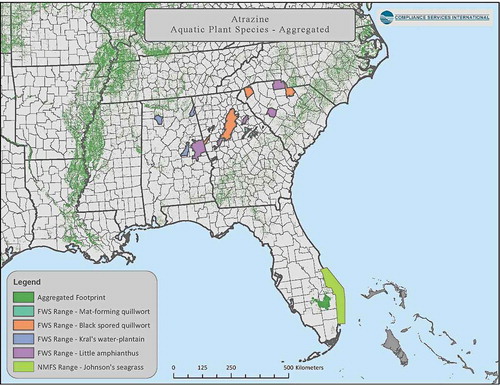
The perennial Potamogeton clystocarpus (Little Aguja pondweed) is found in fewer than 25 sites in a canyon located in the Davis Mountains, Jeff Davis County, Texas⁹. From the distribution of corn acreage in this county, there is a very low likelihood of use of atrazine and therefore exposure in these specific habitats (see SI Section 3.5.1, SI Figures 3–9).

The primarily asexual and perennial herb Sagittaria secundifolia (Kral’s water-plantain) is found in less than four sites in Georgia and predominantly Alabama⁹. There is an overlap of the species-range for Kral’s water-plantain and the crop coverage that is >0.95% (Figure 21 and SI Section 3.5.2, SI Table S3–3).

The seedless, non-flowering perennial herbs Isoetes melanospora (black-spored quillwort) and Isoetes tegetiformans (Mat-forming quillwort) are currently known from 12 or less locations each on rock outcroppings in Georgia, like Amphianthus pusillus⁹. There is a very low likelihood of corn production on rocky outcrops but there is an overlap of the species-range for Mat-forming quillwort and the crop coverage that = 1% (Figure 21 and SI Section 3.5.2, SI Table S3–3).

The asexual seagrass Halophila johnsonii is found in intertidal lagoon-waters along approximately 200 km of coastline in southeastern Florida⁹ (Figure 21 and SI Section 3.5.2, SI Table S3–3). Concentrations of atrazine in marine and estuarine systems are very small (less than 1 µg/L; see Section 3.3.3.2 above) so risks to plants in these systems are very small. Below we summarize the available literature, laboratory, and field, as it relates to the possible risk posed to these species.

4.3 Studies on effects of atrazine on aquatic plants

The effects of atrazine on non-target aquatic plants (including algae) have been studied extensively, with a large set of available data from which to interpret the risk posed to endangered species. Many of these studies have been carried out in the laboratory while others have been conducted in the field, mainly in cosms.

4.3.1 Laboratory studies

A review evaluated the available studies for their strength of methods (Hanson et al. 2019a). Most of these studies measured effects on typical apical endpoints for plants such as growth, biomass, reproduction, and population such as number of cells, etc. Acceptable studies were used to construct species sensitivity distributions (SSDs) for freshwater macrophytes, phytoplankton, and periphyton laboratory data using Caddis Volume 4.¹⁰ In total, seven data-points were plotted for acute exposure responses (taken from Table 10 in Hanson et al. 2019a). This analysis returned an HC5 of 9.6 µg/L for an SSD constructed of EC50s. Moreover, Moore et al. (2017), utilized a dataset generated by USEPA (2012d) based on specific-growth rate (for studies reporting endpoints at multiple time points) to generate a genus sensitivity distribution (GSD). As stated by USEPA (2012d), specific growth rate (SGR) has several advantages, specifically that it is independent of exposure duration, and thus provides a “common currency” across studies. Thus, SGR is directly applicable to addressing effects of time-variable exposures. Based on this dataset (USEPA 2012d), which included EC50s for 21 genera (ranging from 15 to 494 µg/L), Moore et al. (2017) calculated GSD HC5 of 52 µg/L.

Table 4. Highest-ranking peer-reviewed cosm studies with atrazine (overall evaluation score ≥70%)

Reference	Cosm description	Communities monitored	Concentration range^a	Evaluation score
				Relevance	Reliability	Overall^b
(King et al. 2016)	Outdoor streams 20 m long (riffles, glides, pools)	Periphyton	50–150 µg/L (3 pulses)	100%	92%	95%
(Baxter et al. 2011)	Outdoor 12-m^3 ponds	Phytoplankton, periphyton, macrophytes	1–100 µg/L (single addition)	88%	83%	85%
(Knauert et al. 2008; Knauert et al. 2009; Knauert et al. 2010)	Outdoor 10-m^3 ponds	Phytoplankton, macrophytes	70 µg/L (constant)	63%	83%	75%
(McGregor, Solomon, and Hanson 2008)	Outdoor 12-m^3 ponds	Macrophytes	25–250 µg/L (single addition)	63%	83%	75%
(Diana et al. 2000)	Outdoor 90-L pools	Phytoplankton, macrophytes	20–200 µg/L (single addition)	50%	92%	75%
(Hamilton et al. 1987; Hamilton et al. 1988; Herman, Kaushik, and Solomon 1986)	Lake enclosures (limnocorrals), 125 m^3	Phytoplankton, periphyton	80–140 µg/L (2 pulses)	88%	58%	70%
(DeNoyelles, Kettle, and Sinn 1982; DeNoyelles et al. 1989)	0.045-ha (900 m^3) ponds	Phytoplankton	20–500 µg/L (single addition)	88%	58%	70%
(Stay et al. 1985)	4-L jars in incubator; artificial assemblage	Phytoplankton	53–430 µg/L (single addition)	38%	92%	70%

^a“Single addition” means atrazine was applied once and dissipated at a system-specific rate; “pulses” are multiple applications of atrazine separated by intervals of lower exposure; “constant” means atrazine was added as needed to maintain a target concentration.

^bOverall evaluation scores for 108 data points from 39 studies ranged from 25% to 95%. Data abstracted from (Giddings et al. 2018).

Table 5. Risk assessment determination for several listed aquatic vertebrates

Species and reference	Assessment endpoint	Response Determination	Explanation (from the reports cited in column 1)
Barton Springs Salamander (USEPA 2006c).	Survival, growth, and reproduction via direct effects	No effect.	No acute and chronic LOCs are exceeded.
	Indirect effects via reduction of prey (i.e., freshwater invertebrates).	May affect, but not likely to adversely affect.	Acute LOCs are exceeded based on the most sensitive ecotoxicity value for the midge; however, RQs for other dietary items (amphipods, leeches, snails) are less than LOCs. Based on the nonselective nature of feeding behavior in the Barton Springs salamander and low magnitude of anticipated individual effects to all evaluated prey species, atrazine is not likely to indirectly affect the Barton Springs salamander via a reduction in freshwater invertebrate food items. This finding is based on insignificance of effects (i.e., effects to freshwater invertebrates are not likely to result in “take” of a single Barton Springs salamander) and discountability (i.e., the effect to freshwater invertebrates is extremely unlikely to occur given the estimated individual event probability of 1 in 45.5 million).
	Indirect effects via reduction of habitat and/or primary productivity (i.e., aquatic plants).	May affect, but not likely to adversely affect.	Although atrazine use may directly affect individual vascular and non-vascular aquatic plants in Barton Springs, its use within the action area is not likely to adversely affect the Barton Springs salamander via indirect community-level effects to aquatic vegetation. Predicted 14-, 30-, 60-, and 90-day EECs for all modeled atrazine use scenarios within the action area are well below the threshold concentrations representing community-level effects. This finding is based on insignificance of effects (i.e., community-level effects to aquatic plants are not likely to result in “take” of a single Barton Springs salamander).
Shortnose sturgeon, loggerhead turtle; Kemp’s Ridley turtle; green turtle; leatherback turtle (USEPA 2006a).	Survival, growth, and reproduction via direct effects	No effect.	No acute or chronic LOCs for endangered species are exceeded.
	Indirect effects to listed species via reduction of aquatic animals as food supply.	Not likely to adversely affect.	Acute LOCs are exceeded for some animals that are food items of the assessed species. However, the low magnitude of potential effects on any one species, the low number of dietary species potentially affected (indicated by LOC exceedances) relative to the number potentially consumed by the assessed species, and the conservative nature of the EECs used to derive RQs for organisms in flowing water systems suggests that the potential effects to the food supply of the assessed species constitutes an insignificant effect.
	Indirect effects to listed species via reduction of aquatic plants as food items or primary productivity.	Not likely to adversely affect.	No known obligate relationship between the assessed species and any single aquatic plant species exists, and short-term and long-term atrazine concentrations were estimated to be lower than established thresholds for community-level effects to aquatic vegetation.
	Indirect effects to listed species via direct effects on riparian areas required to maintain acceptable water quality and spawning habitat.	Not likely to adversely affect.	Acreage of riparian habitat expected to be sensitive to atrazine is sufficiently low in the Chesapeake Bay watershed such that potential impacts of atrazine to sensitive riparian buffers are not expected to result in a measurable effect to the assessed species that reside in the main stem of the Chesapeake Bay and the Major river systems. Therefore, potential effects to riparian areas from use of atrazine are expected to constitute an insignificant effect .
Alabama Sturgeon (USEPA 2006b).	Survival, growth, and reproduction via direct effects	No effects.	No acute and chronic LOCs are exceeded.
	Indirect effects via reduction of prey (i.e., freshwater invertebrates).	May affect, but not likely to adversely affect.	Individual aquatic plant species within the Alabama River may be affected. However, refined 14-, 30-, 60-, and 90-day EECs, which consider the impact of flow, are well below the threshold concentrations representing community-level effects. In addition, the available monitoring data for the Alabama River show that all detected concentrations are <1 μg/L. This finding is based on insignificance of effects (i.e., community-level effects to aquatic plants are not likely to result in “take” of a single Alabama sturgeon).
	Indirect effects to the Alabama sturgeon via reduction of terrestrial vegetation (i.e., riparian habitat) required to maintain acceptable water quality and spawning habitat.	May affect, but not likely to adversely affect.	Riparian vegetation may be affected because terrestrial plant RQs are above LOCs. However, most of the riparian area adjacent to the current range of the Alabama sturgeon in the Lower Alabama River watershed is forested vegetation, which is not associated with forestry plantation operations. Woody plants are generally not sensitive to environmentally relevant concentrations of atrazine; therefore, effects on shading, streambank stabilization, and structural diversity of riparian areas in the action area are not expected. Although grassy and herbaceous riparian habitat is expected to be sensitive to atrazine effects, the presence of herbaceous riparian areas in the Lower Alabama River watershed is minimal. Therefore, atrazine-related impacts to riparian habitat are expected to have minimal impact on overall sediment loads in the Lower Alabama River watershed, based on surrounding land use and other sources of sedimentation including forestry management practices and annual dredging of navigational channels. This finding is based on insignificance of effects (i.e., atrazine effects to riparian vegetation in the Lower Alabama River cannot be meaningfully measured, detected, or evaluated in the context of a level of effect where “take” of a single Alabama sturgeon would occur).
Pallid sturgeon (USEPA 2007e)	Survival, growth, and reproduction via direct effects.	May affect, but not likely to adversely affect.	Acute and chronic LOCs are exceeded based on screening-level EECs from the non-flowing standard water body. However, flow-adjusted EECs and detected concentrations of atrazine in available monitoring data are less than those shown to cause adverse acute and chronic effects in freshwater fish.
	Indirect effects via reduction of prey (i.e., freshwater fish and invertebrates).	May affect, but not likely to adversely affect.	Chronic LOCs are exceeded based on screening-level EECs, refined measures of exposure (i.e., 21-day flow adjusted EECs and available monitoring data) are well below levels that result in chronic effects for the most sensitive freshwater invertebrate species.
	Indirect effects via reduction of habitat and/or primary productivity (i.e., aquatic plants).	May affect, but not likely to adversely affect.	Individual aquatic plant species within the Missouri, Mississippi, and Atchafalaya Rivers may be affected. However, 14-, 30-, 60-, and 90-day EECs, are well below the threshold concentrations representing community-level effects. The available monitoring data for large rivers where the sturgeon occurs indicate that peak detected concentrations are less than the 14-day threshold concentration representing aquatic community-level impacts.
	Indirect effects via reduction of terrestrial vegetation (i.e., riparian habitat) required to maintain acceptable water quality.	Direct effects to forested riparian vegetation: May affect, but not likely to adversely affect Direct effects to grassy/herbaceous riparian. vegetation: Likely to adversely affect	Riparian vegetation may be affected because terrestrial plant RQs are above LOCs. However, woody plants are generally not sensitive to environmentally relevant concentrations of atrazine; therefore, effects on shading, streambank stabilization, and structural diversity of riparian areas are not expected. There is potential for atrazine to affect the spawning habitat via impacts on riparian vegetation depends primarily on the extent of potentially sensitive (herbaceous and grassy) riparian areas and their impact on water quality in the rivers where the sturgeon is known to occur. Because woody plants are generally not sensitive to atrazine at expected exposure concentrations, riparian areas which have predominantly forested vegetation containing woody shrubs and trees are not likely to be impacted by atrazine use.
Topeka Shiner USEPA (2009b)	Survival, growth, and reproduction via direct effects.	Acute effects -No effect.	No acute LOCs exceeded based on LC50 for the most sensitive freshwater fish.
		Chronic effects -Likely to adversely affect.	RQs were up to 1.3 to 1.6 based on maximum labeled application rates.
	Indirect effects via potential effects on aquatic plants.	Likely to adversely affect.	Community level effects are exceeded based on PRZM/EXAAMS based on labeled application rates for corn and fallow and forestry uses.
	Indirect effects via direct effects to aquatic and terrestrial invertebrates as food items.	Not likely to adversely affect.	Effects on aquatic and terrestrial invertebrate food items is low.
	Indirect effects via direct effects to other fish needed for spawning habitat and diet.	Not likely to adversely affect.	The potential magnitude of effect to fish is expected to be low.
	Indirect effects via direct effects to individuals via reduction of terrestrial vegetation to maintain acceptable water quality.	Likely to adversely affect due to direct effects on riparian vegetation.	Grassy and herbaceous vegetation may be sensitive to atrazine. Assumed this may be potentially adverse to the Topeka shiner.

Table 6. Endpoints characterized in the quantitative weight of evidence assessment of the effects of atrazine on aquatic vertebrates

Apical Endpoint	Response	Relevance^a	Quality of Methods^a
Development	Hatching of eggs in fish and amphibians.	0.14 ± SE 0.10	2.24 ± SE 0.11
	Time to hatching in amphibians	0.00 ± SE .00	2.13 ± SE 0.66
	Time to, or age at metamorphosis in amphibians.	0.12 ± SE .08	1.72 ± SE 0.12
Survival	Survival of fish and amphibians after short-term exposures to atrazine.	0.04 ± SE .02	1.65 ± SE 0.06
	Survival of fish and amphibians after long-term exposures to atrazine.	0.15 ± SE .1	2.00 ± SE 0.13
	Successful development in fish and metamorphosis in amphibians.	0.12 ± SE .07	1.86 ± SE 0.11
Growth	Weight and/or size of fish, amphibians.	0.1 ± SE .03	1.74 ± SE 0.08
	Deformities in fish and amphibians	0.01 ± SE .01	1.86 ± SE 0.09
Reproduction	Sex ratios in fish and amphibians	0.06 ± SE .04	1.96 ± SE 0.12
	Gonad-somatic index in fish and amphibians.	0.11 ± SE .06	2.33 ± SE 0.12
	Production of eggs in fish.	0.06 ± SE .03	2.62 ± SE 0.16

^aScores based on assessments in (Van Der Kraak et al. 2014) and (Hanson et al. 2019b).

Table 7. No observed effects concentrations for atrazine in chronic studies on reproduction in fish

Study design	Species	NOAEC (µg/L)	Reference	Score for QoM^a
Fish Full Lifecycle	Brook Trout (Salvelinus frontinalis)	65	(Macek et al. 1976)	2.2
	Bluegill sunfish (Lepomis macrochirus)	95	(Macek et al. 1976)	2.8
	Fathead minnow (Pimephales promelas)	213	(Macek et al. 1976)	2.6
	Fathead minnow (P. promelas)	250	(Dionne 1992)	3.2
Fish Short-Term Reproduction Assay	Japanese medaka (O. latipes)	0.5	(Papoulias et al. 2014)	2.4
	Fathead minnow (P. promelas)	0.5	(Tillitt et al. 2010)	2.4
	Fathead minnow (P. promelas)	105	(Syngenta 2017b)	3.8
	Fathead minnow (P. promelas)	223.7	(USEPA 2005)	2.8
	Japanese medaka (Oryzias latipes)	244	(Syngenta 2017 c)	3.6
	Japanese medaka (O. latipes)	>53	(Syngenta 2015)	3.4
	Fathead minnow (P. promelas)	>50	(Bringolf, Belden, and Summerfelt 2004)	2.2

^aQoM = quality of methods from the QWoE assessments in (Hanson et al. 2019b; Van Der Kraak et al. 2014). Because multiple different responses were measured in these studies, it is not possible provide a mean score for relevance; however, these individual scores are provided in the supplemental information (SI) of the QWoE assessments referenced above.

Table 8. Occurrence of listed terrestrial invertebrates and designated critical habitat in counties with more than 0.95% overlap between species-range and acreage of corn, sorghum, and sugarcane

Species name	Common name	Taxon	Habitat^a	Feeding guild	Exposure via diet	Critical habitat
Anaea troglodyta floridalis	Florida leafwing butterfly	Insect	T	Coprophagous, frugivore, nectarivore, herbivore	Possibly
Batrisodes texanus	Coffin Cave mold beetle	Insect	TC	Fungivore	None
Batrisodes venyivi	Helotes mold beetle	Insect	T	Fungivore	None
Cicurina baronia	Robber Baron Cave meshweaver	Arach.	TC	Invertivore	None
Cicurina madla	Madla Cave meshweaver	Arach.	TC	Invertivore	None
Cicurina venii	Braken Bat Cave meshweaver	Arach.	TC	Invertivore	None
Cicurina vespera	Government Canyon Bat Cave meshweaver	Arach.	TC	Invertivore	None
Hesperia dacotae	Dakota skipper	Insect	T	Nectivore, herbivore	Possibly
Heterelmis comalensis	Comal Springs riffle beetle	Insect	A	Invertivore?	Unknown
Icaricia icarioides fender	Fender’s blue butterfly	Insect	T	Nectivore, herbivore	Possibly
Microhexura montivaga	Spruce-fir moss spider	Arach.	T	Invertivore	None
Neoleptoneta microps	Government Canyon Bat Cave spider	Arach.	T	Invertivore	None
Neoleptoneta myopica	Tooth Cave spider	Arach.	T	Invertivore	None
Nicrophorus americanus	American burying beetle	Insect	T	Carrion	None
Rhadine exilis	[no common name] cave dwelling beetle	Insect	TC	Fungivore	None
Rhadine infernalis	[no common name] cave dwelling beetle	Insect	TC	Fungivore	None
Somatochlora hineana	Hine’s emerald dragonfly	Insect	T & A	Invertivore	None	✓
Strymon acis bartrami	Bartram’s hairstreak butterfly	Insect	T	Nectivore, herbivore	Possibly
Stygoparnus comalensis	Comal Springs dryopid beetle	Insect	S & A	Fungivore?	None
Tartarocreagris texana	Tooth Cave pseudoscorpion	Arach.	TC	Invertivore	None
Texella cokendolpheri	Cokendolpher Cave harvestman	Arach.	TC	Invertivore	None
Texella reddelli	Bee Creek Cave harvestman	Arach.	TC	Invertivore	None
Texella reyesi	Bone Cave harvestman	Arach.	TC	Invertivore	None

^aT = terrestrial, A = aquatic, S = subterranean, TC = terrestrial cave dweller

Data from https://www.fws.gov/, http://explorer.natureserve.org & https://ecos.fws.gov/ipac/

Table 9. Occurrence of listed mammals and associated designated critical habitat in counties with more than 0.95% overlap between species-range and acreage of corn, sorghum, and sugarcane

Species name	Common name	Habitat^a	Feeding guild	Exposure via diet	Critical habitat
Antilocapra americana sonoriensis	Sonoran pronghorn	T	Herbivore	Possibly
Brachylagus idahoensis	Columbia Basin pygmy rabbit	T	Herbivore	Possibly
Canis lupus	Gray wolf	T	Carnivore	None	✓
Canis rufus	Red wolf	T	Carnivore	None
Corynorhinus townsendii ingens	Ozark big-eared bat	TC	Invertivore	None
Corynorhinus townsendii virginianus	Virginia big-eared bat	TC	Invertivore	None
Cynomys parvidens	Utah prairie dog	T	Herbivore	Possibly
Eumops floridanus	Florida bonneted bat	TC	Invertivore	None
Glaucomys sabrinus coloratus	Carolina northern flying squirrel	T	Frugivore, granivore, invertivore	Possibly
Gulo gulo luscus	North American wolverine	T	Carnivore	None
Herpailurus yagouaroundi cacomitli	Gulf Coast jaguarundi	T	Carnivore	None
Leopardus pardalis	Ocelot	T	Carnivore	None
Lynx canadensis	Canada lynx	T	Carnivore, carrion	None	✓
Microtus pennsylvanicus dukecampbelli	Florida salt marsh vole	T	Herbivore	Possibly
Mustela nigripes	Black-footed ferret	T	Carnivore	None
Myotis grisescens	Gray bat	TC	Invertivore	None
Myotis septentrionalis	Northern long-eared bat	TC	Invertivore	None
Myotis sodalis	Indiana bat	TC	Invertivore	None	✓
Odocoileus virginianus leucurus	Columbian white-tailed deer	T	Herbivore	Possibly
Panthera onca	Jaguar	T	Carnivore	None
Peromyscus polionotus allophrys	Choctawhatchee beach mouse	T	Granivore, invertivore	Possibly
Peromyscus polionotus ammobates	Alabama beach mouse	T	Granivore, invertivore	Unlikely	✓
Peromyscus polionotus niveiventris	Southeastern beach mouse	T	Frugivore, granivore, invertivore	Possibly
Peromyscus polionotus phasma	Anastasia Island beach mouse	T	Granivore, invertivore	Unlikely
Puma (=Felis) concolor coryi	Florida panther	T	Carnivore	None
Thomomys mazama pugetensis	Olympia pocket gopher	T	Granivore, invertivore	Possibly
Thomomys mazama tumuli	Tenino pocket gopher	T	Granivore, invertivore	Possibly
Thomomys mazama yelmensis	Yelm pocket gopher	T	Granivore, invertivore	Possibly
Trichechus manatus	West Indian manatee	A	Herbivore	None
Zapus hudsonius preblei	Preble’s meadow jumping mouse	T	Frugivore, granivore, invertivore	Possibly	✓

^aT = terrestrial, A = aquatic, S = subterranean, TC = terrestrial cave dweller

Data from https://www.fws.gov/, http://explorer.natureserve.org & https://ecos.fws.gov/ipac/

Table 10. Occurrence of listed birds and associated designated critical habitat in counties with more than 0.95% overlap between species-range and acreage of corn, sorghum, and sugarcane

Species name	Common name	Habitat^a	Feeding guild	Exposure via diet	Critical habitat
Ammodramus maritimus mirabilis	Cape Sable seaside sparrow	T	Granivore, invertivore	Possibly
Ammodramus savannarum floridanus	Florida grasshopper sparrow	T	Granivore, invertivore	Possibly
Aphelocoma coerulescens	Florida scrub-jay	T	Carnivore, Granivore, Invertivore	Possibly
Brachyramphus marmoratus	Marbled murrelet	T & A	Piscivore	None
Calidris canutus rufa	Red knot	T	Granivore, invertivore	Possibly
Campephilus principalis, possibly extinct	Ivory-billed woodpecker	T	Invertivore	None
Centrocercus minimus	Gunnison sage-grouse	T	Herbivore, invertivore	Possibly	✓
Charadrius melodus	Piping plover	T & A	Invertivore	None	✓
Charadrius nivosus nivosus	Western snowy plover	T & A	Invertivore	None
Coccyzus americanus	Yellow-billed cuckoo	T	Invertivore	None	✓
Dendroica chrysoparia	Golden-cheeked warbler	T	Invertivore	None
Empidonax traillii extimus	Southwestern willow flycatcher	T	Invertivore	None
Eremophila alpestris strigata	Streaked horned lark	T	Granivore, invertivore	Possibly
Falco femoralis septentrionalis	Northern Aplomado falcon	T	Carnivore, invertivore	None
Grus americana	Whooping crane	T & A	Carnivore, frugivore, granivore, invertivore, piscivore	Possibly
Grus canadensis pulla	Mississippi sandhill crane	T & A	Carnivore, granivore, herbivore, invertivore	Possibly
Gymnogyps californianus	California condor	T	Carnivore, carrion	None
Laterallus jamaicensis ssp. jamaicensis	Eastern black rail	T	Granivore, invertivore	Possibly
Mycteria americana	Wood stork	T & A	Piscivore	None
Numenius borealis, presumed extirpated	Eskimo curlew	T & A	Frugivore, invertivore	Possibly
Picoides borealis	Red-cockaded woodpecker	T	Invertivore	None
Polyborus plancus audubonii	Audubon’s crested caracara	T	Carnivore, invertivore	None
Pterodroma hasitata	Black-capped petrel	T	Invertivore	None
Rallus longirostris yumanensis	Yuma clapper rail	T & A	Invertivore, piscivore	None
Rostrhamus sociabilis plumbeus	Everglade snail kite	T	Invertivore	None
Sterna antillarum	Least tern	T & A	Piscivore	None
Sterna antillarum browni	California least tern	T & A	Invertivore, piscivore	None
Sterna dougallii dougallii	Roseate tern	T & A	Piscivore	None
Strix occidentalis caurina	Northern spotted owl	T	Carnivore	None
Strix occidentalis lucida	Mexican spotted owl	T	Carnivore	None	✓
Tympanuchus cupido attwateri	Attwater’s greater prairie-chicken	T	Frugivore, granivore, herbivore, invertivore	Possibly	✓
Vermivora bachmanii	Bachman’s warbler	T	Invertivore	None

^aT = terrestrial, A = aquatic, S = subterranean, TC = terrestrial cave dweller

Data from https://www.fws.gov/, http://explorer.natureserve.org & https://ecos.fws.gov/ipac/

For estuarine/marine species, exposures, and consequent risks, are generally lower relative to freshwater environments. For estuarine/marine environments mean atrazine concentrations were found to be highest at primary (i.e., agricultural drainage ditch) sites, which were ~9 times higher (8.52 ± 1.79 μg/L) than at bay sites (0.92 ± 0.19 μg/L) along the mid-Texas coast (Pennington et al. 2001). Additionally, as part of the Chesapeake Bay Program (CBP), the highest peak concentration of atrazine detected (30 µg/L) was found in a tributary on the Eastern Shore, while the 99th, 95th, 90th, 75th, and 50th centile values were 2.5, 0.5, 0.28, 0.1, and 0.05 µg/L, respectively (USEPA 2006a). Thus, potential exposures for estuarine/marine organisms to atrazine are considerably lower than corresponding freshwater counterparts. This indicates that the risk posed to listed species of aquatic plants based on current exposure would be negligible with no anticipated direct and therefore no expected indirect effects (as discussed below).

No study, to our knowledge, has examined the effects of atrazine to listed species. There has been some work with related marine seagrasses (Zostera muelleri, Zostera marina, Halophila ovalis, and Halodule uninervis) that could be considered a surrogate for Halophila johnsonii. As reported by Hanson et al. (2019a), many of the available studies on marine macrophytes were methodologically weak (and not considered suitable for ERA). For apical responses, reported LOECs ranged from 100 to 1900 µg/L, while concentrations causing inhibition of photosystem II (the site of action of atrazine and a biomarker response), ranged from 2 to 10 μg/L. Finally, the laboratory evidence that aquatic primary producers can recover from pulsed or transient exposures in the field, which are common in lotic systems (see Section 3.3.3.1 above), is also extensive (see Section 2.4).

4.3.2 Field and semi-field studies

4.3.2.1 Scope and history of the atrazine cosm database

Atrazine has been studied extensively in cosms (model aquatic ecosystems–microcosms and mesocosms) to obtain data on responses of populations, communities, and ecosystems under quasi-natural conditions. More than 40 cosm studies on atrazine have been reported in the peer-reviewed literature. Experimental systems have ranged in size and complexity from benchtop flasks with species introduced from laboratory cultures to full-scale farm ponds and lake enclosures. The body of evidence from cosm studies with atrazine has been used to provide insights into its ecological effects (Giddings et al. 2005; Solomon et al. 1996) and as the basis for regulatory safety criteria (USEPA 2007c, 2016). Here we summarize those findings and their relevance to listed species.

Giddings et al. (2018) summarized the history and scope of the atrazine cosm-database from its origins during FIFRA Reregistration (USEPA 2003b) through its most recent implementation in FIFRA Registration Review (USEPA 2016). Moore et al. (2017) and Giddings et al. (2018) conducted independent data quality reviews of the atrazine cosm studies and reached similar conclusions about which studies are most relevant and reliable for risk assessment. No study explicitly examined the response of listed species, but many of the studies provided knowledge about ecological responses to atrazine that are relevant to the assessment of listed species. The studies ranked highest by Giddings et al. (2018), which were the source of 35 data points out of 108 in the database, are summarized in Table 4 (a data point is defined as the response of phytoplankton, periphyton, or macrophytes to a single experimental treatment in a single study). The findings from these high-quality studies are described below and their implications for listed species discussed.

4.3.2.2 Observed direct effects on phytoplankton and periphyton

Data from the highest quality cosm studies show that atrazine has little or no effect on phytoplankton and periphyton at concentrations as great as 150 µg/L. Exposure to atrazine concentrations from 50 to 150 µg/L (treatment repeated three times) had no effect on phytoplankton biomass or community structure and no effect on community structure of periphyton, while periphyton biomass was briefly reduced but recovered to control values after the last treatment (King et al. 2016). Concentrations from 1 to 100 µg atrazine/L had no effect on ash-free dry weight of phytoplankton or periphyton (Baxter et al. 2011). Concentration of chlorophyll in phytoplankton did not change at 20 µg/L but increased at 200 and 2000 µg/L (Diana et al. 2000); this was interpreted as a response to nutrients and light made available by decay and removal of macrophytes at these high concentrations.

Knauert et al. (2008) measured the inhibition of photosystem II directly in communities of phytoplankton in cosms using quantum yield and reported approximately 50% reduction within 2 days at 70 µg/L, with the effect continuing throughout a 34-d constant exposure period. Total abundance of phytoplankton in treatments declined but recovered to control levels after day-40 (Knauert et al. 2009). Atrazine affected phytoplankton succession; diversity in treated cosms exceeded controls during the treatment period and was similar to controls for 5 months post-treatment (Knauert et al. 2009).

In earlier studies in lake enclosures (Hamilton et al. 1987, 1988; Herman, Kaushik, and Solomon 1986), effects on periphyton and phytoplankton biomass and decreases in abundance of some algal populations were observed at concentrations from 80 to 140 µg/L. Productivity was also measured by fixation of ¹⁴CO₂. In one experiment the enclosures were treated twice with 100 µg/L atrazine (Herman, Kaushik, and Solomon 1986). Treatments were 6 weeks apart and, after both treatments, compensatory responses were observed. Numbers of some species of Chloraphyta decreased while others increased. Bacillariophyceae dominated the algal biomass in the treated cosms after the second application but overall biomass was not adversely affected.

The experimental systems at the University of Kansas (DeNoyelles et al. 1989; DeNoyelles, Kettle, and Sinn 1982) were realistic constructed ponds that became the prototypes for the FIFRA cosm guideline (USEPA 1996). As the series of exploratory studies proceeded over several years, experimental designs and techniques evolved. While the systems were rated high for realism, the results were often inconsistent or obscured by complicating factors and were generally rated low for reliability (quality) (Giddings et al. 2018). However, two of the eight data points from these studies received overall quality ratings of 70%. These were for phytoplankton photosynthesis (measured by fixation of ¹⁴CO₂) and biomass at 20 µg atrazine/L and 500 µg atrazine/L in the first study year (DeNoyelles, Kettle, and Sinn 1982). The response observed at 500 µg/L was a clear effect but results at 20 µg/L were inconsistent and a phytoplankton bloom that occurred in one of the two control replicates complicated interpretation. These results were discussed in detail by Solomon et al. (1996) and Giddings et al. (2005), who concluded that the 20 µg/L data point is properly scored “no effect,” an opinion supported by the SAP (USEPA 2012b) but not implemented in EPA’s latest analysis (USEPA 2020b).

Stay et al. (1985) measured the effect of a wide range of atrazine concentrations (53 to 5000 µg/L) on phytoplankton communities in small, highly artificial cosms (4-L flasks containing artificial medium and algal inocula from single-species cultures). The study made up in quality what it lacked in relevance and thus achieved an overall score of 70%. Chlorophyll, fixation of ¹⁴CO₂, and production and respiration (by dissolved oxygen, corrected for diffusion) were monitored. Fixation of ¹⁴CO₂ was reduced at all concentrations from the first measurement (4 days after treatment with atrazine). An immediate response of algal photosynthesis to atrazine exposure is consistent with atrazine’s mode of action. A consistent concentration–response relationship was observed.

Overall, in the high-quality cosm studies, atrazine concentrations up to 30 µg/L, and in some cases as great as 200 µg/L, had no effect on phytoplankton or periphyton. Effects were observed at concentrations of 50 µg/L and greater in most cases. Recovery of phytoplankton and periphyton communities in atrazine cosms is discussed below. Based on these results, we would anticipate no risk of adverse effects on phytoplankton and periphyton except under extremely rare exposure conditions (see Section 3.3.3.1) and indirect effects would not be expected. By analogy, this conclusion is applicable to listed species.

4.3.2.3 Observed direct effects on macrophytes

The highest quality study that included measurement of the effects of atrazine on macrophytes (Baxter et al. 2011) showed that growth of potted macrophytes (Myriophyllum spicatum and Elodea canadensis) was reduced at 100 µg/L atrazine but unaffected at 1 to 30 µg/L. McGregor, Solomon, and Hanson (2008) conducted what was essentially a large outdoor toxicity test in systems similar to Baxter’s, with results presented as EC10, EC25, and EC50 values for growth of M. spicatum and E. canadensis–data that are difficult to compare with other cosm results. McGregor, Solomon, and Hanson (2008) also measured productivity of macrophytes (based on dissolved oxygen) and reported effects at 100 and 250 µg/L but not at 25 and 50 µg/L. In a similar study in much smaller (90-L) cosms, Diana et al. (2000) found no effect of atrazine on biomass of macrophytes at 20 µg/L but a significant reduction in biomass and mortality at 200 and 2000 µg/L. Knauert et al. (2010) measured the effect of 70 µg atrazine/L on photosynthetic efficiency in macrophytes and observed reductions 2 days after treatment with recovery by day 12 and no effect on growth rate (the response was scored as No Effect by Giddings et al. (2005; 2018)). Thus, the high-quality cosm studies showed no effects of atrazine on macrophytes at concentrations up to 70 µg/L, and effects at 100 to 250 µg/L.

Effects of atrazine on macrophytes were also measured in some of the studies in Kansas cosms. However, responses of macrophytes in these studies were particularly difficult to interpret due to factors such as declining water levels and the introduction of herbivorous fish, as well as the difficulty of nondestructive monitoring and the high spatial heterogeneity of macrophyte growth and abundance in the field (Giddings et al. 2005). Effects were reported at 100 to 500 µg/L. Responses of macrophytes at 20 µg/L were ambiguous. None of the data for macrophytes from the Kansas studies (DeNoyelles et al. 1989; DeNoyelles, Kettle, and Sinn 1982) met the 70% overall quality criterion for inclusion in this discussion. Based on these results, we anticipate no risk of adverse effects of atrazine on listed aquatic plant species, except under extremely rare exposure conditions (see Section 3.3.3.1 above).

4.3.2.4 Recovery of plant populations and communities

Most of the high-quality studies measured plant community metabolism (e.g., photosynthesis), either directly (using fixation of ¹⁴CO₂), as fluorescence quantum yield, or inferred from dynamics of dissolved oxygen. A common observation was that these parameters responded quickly to exposure, usually in a clear concentration-response manner, and that they recovered almost immediately when concentrations of atrazine declined (Diana et al. 2000; King et al. 2016; McGregor, Solomon, and Hanson 2008; Stay et al. 1985). Structural parameters such as biomass (or a surrogate such as concentration of chlorophyll) and community-composition tend to respond more slowly, and these ecological effects persisted longer than direct effects on photosynthesis (Knauert et al. 2009).

Conclusions from atrazine cosm studies

USEPA (USEPA 2007c, 2012b, 2016) used the observed relationship between atrazine exposure (time-series chemograph) and ecological response (effect or no effect) for each cosm data point as the basis for derivation of a level of concern (LOC) for protection of aquatic life. The analytical approach evolved over time and was found to be highly sensitive to both the models used and the interpretation of individual data points (Giddings et al. 2005, 2018; Moore et al. 2017). Using USEPA’s methods and versions of the database that accounted for data quality, Moore et al. (2017) and Giddings et al. (2018) derived similar LOCs of approximately 20 µg/L.

However, a more direct approach for deriving a LOC from the cosm data is a “simple and transparent time and concentration-based LOC” as recommended by the 2009 SAP (USEPA 2009a). Throughout many versions of the atrazine cosm databases, effect or no-effect results were arrayed on axes representing initial atrazine concentration and duration of exposure. When the 35 data points from the highest quality studies (i.e., those with overall data quality scores of 70% or greater) are portrayed in this way (Figure 22), it can be seen that atrazine did not affect plant communities when initial concentrations of atrazine were smaller than 50 µg/L, regardless of exposure duration.

Figure 22. Effect scores as a function of initial atrazine concentration and exposure duration, using data with overall evaluation scores of 70% or greater. From Giddings et al. (2018). Dashed vertical line indicates an initial atrazine concentration of 50 µg/L

The cosms provide abundant evidence of the capacity of aquatic plant communities to recover quickly from the temporary effects of atrazine exposure. When atrazine concentrations dissipate, photosynthesis resumes. Plant communities appear to tolerate such temporary reductions in photosynthesis (as would also occur due to natural fluctuations in light via cloud cover, turbidity, and depth of water), and structural parameters (e.g., biomass, species diversity) may be unaffected in the long run.

The body of cosm data for atrazine supports the conclusion that aquatic vascular and non-vascular plants are at negligible risk except at concentrations of 50 µg/L or greater, which rarely occur in the field (see Section 3.3.3.1 above). Photosynthesis, the most sensitive plant endpoint, recovered rapidly after episodic exposure to atrazine. Indirect effects on aquatic animals are unlikely except at atrazine concentrations that cause severe damage to aquatic plants (200 µg/L or greater). In conclusion, the risk of atrazine adversely affecting listed aquatic plants is negligible.

4.4 Population modeling

Population models are a recommended methodology for Step-3 assessments (National Academy of Sciences 2013), as they can integrate information on relevant species and chemical/exposure scenarios for a more comprehensive assessment of risk. To our knowledge, there are currently no existing population models that can be readily used for assessing risks to the listed aquatic macrophytes (Forbes and Galic 2016).

However, there are some important developments in modeling risks to aquatic primary producers for regulatory purposes. The European Food Safety Agency (EFSA) panel on plant production products has recently reviewed several models and published their opinion on their acceptability for use in aquatic risk assessments (EFSA 2018). EFSA’s assessment included models of phytoplankton (Raphidocelis subcapitata and Desmodesmus subspicatus) and macrophyte species (Lemna sp., Myriophyllum sp.). The panel reviewed model structure, quality and adequacy of data used for model calibration and validation and provided recommendations for future experimental needs. The macrophyte models reviewed in the opinion could potentially be modified to represent listed macrophyte species, but the amount of necessary modification would depend on the differences in life-history, physiology, and ecological characteristics between modeled and listed species. The main challenge to this would be gathering additional empirical data for model development and testing due to the regulatory constraints on handling listed species.

Ecosystem modeling has been applied to assess potential risks from exposure to atrazine for non-listed aquatic species. The Comprehensive Aquatic System Model (CASM) represents generic or specific aquatic ecosystems by including relevant physical-chemical factors with relevant ecological interactions, including competition, grazing, and predation (Bartell et al. 2013). The model has been modified to represent a generic lower-order Midwestern stream and was applied to quantify potential effects from exposure to realistic concentrations of atrazine (CASM_ATZ) (Bartell et al. 2013). In this specific study, exposures for atrazine were derived from three vulnerable watersheds which were a part of the AEMP (Prenger et al. 2009). Population- and community-level effects were expressed as changes in biomass and changes in the Steinhaus similarity index (Legendre and Legendre 2012), which tracks differences in relative distributions of biomass among all modeled populations. Simulations of exposure to monitored atrazine exposures in the three vulnerable watersheds (included via chemographs) showed the median community-level maximum 30-d average similarity index to be between 0.09% and 2.52% change from baseline (control) conditions. This study did not specifically model listed species but included several species of aquatic vascular plants including Vallisneria, Myriophyllum, Ceratophyllum, Elodea, Lemna, and Potamogeton as well as five populations of diatoms, seven of chlorophytes, and six of cyanophytes, as well as one euglenoid and one cryptophyte population. Listed and non-listed species of terrestrial plants have been shown not to differ significantly in their demographic traits or their responses to stressors (Christl et al. 2018; Rueda-Cediel et al. 2019), neither were any differences in sensitivity to crop protection products found in crop and wild species of terrestrial plants. We thus assume that the diversity of aquatic plants included in the ecosystem model is representative of the ecology and responses of listed aquatic plant species. These results indicate that exposure to atrazine in aquatic environments poses no discernable risk to the whole ecosystem, which includes multiple species of listed and non-listed aquatic plants.

4.5 Assessment of risks under ESA – direct effects

Of the seven currently listed species of aquatic plants in the United States with a significant water phase as part of their life history, the current data indicate little to no risk posed by atrazine to their ability to survive, grow, or reproduce. The freshwater species are all located in areas isolated from atrazine use and agriculture in general, meaning exposures will be minimal to non-existent.

Of the six listed freshwater species, included in the assessment, two are monocots (Potamogeton clystocarpus and Sagittaria secundifolia), two are dicots (Amphianthus pusillus and Nasturtium gambelii) and two (Isoetes melanospora and Isoetes tegetiformans) are pteridophytes (vascular plants that reproduce via spores). The best available laboratory data for monocots and dicots indicate that significant adverse effects are unlikely at current measured environmental concentrations of atrazine, and that recovery from exposures, should they occur, is rapid. While there are no toxicity data for pteridophytes exposed to atrazine, there is no reason to believe these species would be more sensitive than dicots or monocots, as the mode and site of action is conserved across groups.

The seagrass Halophila johnsonii is a monocot found predominantly in intertidal waters along the coastline of southeastern Florida. The likelihood of exposure is very low (see Section 3.3.3.2 above), and data from closely related seagrass species indicate that effects are highly unlikely, with 72-h EC10, EC20, and EC50 values for inhibition of effective quantum yield of PSII in Zostera muelleri and Halodule uninervis ranging from 13 to 48 μg/L (Jones and Winchell 1984). Similar biochemical responses were reported in Zostera marina, where adenylate energy charge was affected by short (6 h) exposures to 10 and 100 µg atrazine/L but increased with longer (21-day) exposures at the same concentrations. These concentrations are orders of magnitude greater than what was observed in saltwater systems (see Section 3.3.3.2 above) and represent a physiological response at the mode of action, and not an apical response, making these data for effects highly protective. When considering exposure in marine ecosystems, the risk to Halophila johnsonii is de minimis. The lack of high-quality data for marine species that reported ecologically relevant apical responses is a gap that may need to be addressed.

For phytoplankton, periphyton, or macrophyte populations and communities, there is little evidence that exposure to atrazine results in a direct effect on growth and development, abundances, or structure at current environmental concentrations. The cosm database is consistent in showing that environmentally relevant concentrations of atrazine do not have significant adverse effects on aquatic primary producers, and that recovery, when changes are observed, is rapid, in line with laboratory studies.

4.6 Assessment of risks under ESA – plant-related indirect effects

There are three major pathways by which atrazine could mediate indirect ecological effects on listed species in aquatic ecosystems. The first would be for an adverse direct effect on primary producers, which would result in an indirect effect on listed animal or plant species with a significant or obligate relationship with the affected aquatic plants. The second would be for atrazine to significantly modify the community composition of aquatic primary producers (e.g., through a shift from a clear water macrophyte dominated state to a turbid state, dominated by phytoplankton (Jeppesen et al. 2012), such that the listed species would no longer be able to compete or access resources effectively. The third mechanism, that is in part an extension of the second, would be for a significant change on higher-level organisms that feed or access the organism as a resource (e.g., an increase in snails resulting in an increase in grazing pressure or a change in abundance of tadpoles that graze on periphyton as hypothesized by Rohr et al. 2008a) and has been reported in other papers unrelated to atrazine (Burlakova et al. 2009; Kupferberg 1997; Pieczyńska 2003).

As noted above, largely because of lack of exposure, there is de minimis risk of direct effects on listed species of aquatic plants at this time. To our knowledge, there are no listed species of animals with a significant or obligatory relationship with any listed aquatic primary producers. However, indirect effects on listed herbivores could theoretically result from direct effects on aquatic plants that are not listed as endangered (see Section 5.2.3 below).

Atrazine, as an herbicide, has the theoretical potential to shift species dominances in an aquatic ecosystem (e.g., transition from a macrophyte-dominated system to one dominated by phytoplankton, or vice versa, depending on relative sensitivity of organisms). If macrophytes are significantly more sensitive atrazine than phytoplankton and/or periphyton, then the loss of a dominant macrophyte could free up nutrients and other resources for phytoplankton to drive primary production, depending on the duration of the response. This may then result in an environment with lower availability of light, less dissolved nutrients for resumed macrophyte growth upon cessation of exposure to atrazine, and enhanced epiphytic growth, further challenging a vulnerable endangered macrophyte. Currently, there is no strong evidence from laboratory or cosm studies that macrophytes are significantly more sensitive to atrazine than phytoplankton or periphyton, or that exposures exceed the concentration or duration to induce a significant effect (see Section 3.3.3.1 above). Therefore, this mechanism of indirect effects on macrophytes, endangered or otherwise, can be excluded.

The third mechanism by which a pesticide could have an impact on a listed aquatic primary producer is through a shift in higher-level organisms (herbivores) that influence the growth, development, and reproduction of the listed species. This could be through a direct effect on the higher-level organism (e.g., a decrease in their abundance, or a change in their behavior) or via an indirect effect (such as those described above) that results in change. As it relates to the first mechanism, there is no strong evidence of direct effects of atrazine in animals that might feed or otherwise interact adversely with listed species (see Section 5.3.3 below) at environmentally relevant concentrations. This includes organisms that might graze (e.g., snails, amphibian tadpoles). Therefore, this mechanism of indirect effects on macrophytes, endangered or otherwise, can be excluded at this time. The other route by which this mechanism may have an influence is through a change in dominance of primary producers driving a shift in grazers, which in turn could influence the viability of a listed species. This has been proposed as it relates, for example, to snails as a vector of amphibian parasites increasing due to greater growth of periphyton (occurring as a result of direct effects on macrophytes as described above) as a result of exposure to atrazine (Rohr et al. 2008b), and therefore the likelihood of adverse effects on vulnerable frog populations (see Section 5.3.3 below for more details). It is reasonable to assume that an increase in grazers of macrophytes, such as certain snails, could result in a decrease in growth of macrophytes, development, and overall success of macrophytes as a whole, and endangered macrophytes especially (Burlakova et al. 2009; Wong, Kwong, and Qiu 2009). In the study by Baxter et al. (2011), measures were taken of macrophyte, phytoplankton, and periphyton biomass, growth, and fecundity of snails (Physella spp, caged and uncaged) and uncaged pond snails (Stagnicola elodes). Except for declines in biomass of macrophytes at the highest treatment level, no consistent relationships were found between concentrations of atrazine and any measured parameter. Comparison of these results with previous findings highlights the variability of responses to atrazine exposure between similarly constructed freshwater communities, even at concentrations up to 20-times greater than sustained environmental levels. An examination of the cosm literature does not support a shift in dominance of primary production, or evidence of changes in grazer abundances, at environmentally relevant concentrations (see Section 5.3.3). Therefore, this mechanism of indirect effects on macrophytes, endangered or otherwise, can be excluded.

4.7 Strengths and uncertainties

There is a large body of high-quality literature and data (laboratory and field) to draw from to interpret the potential risk posed by atrazine to listed aquatic primary producers. The mechanism of action in aquatic plants and exposures in aquatic ecosystems are also well understood and characterized. This results in a low level of uncertainty and/or data gaps as to the potential risks posed by atrazine overall. Still, for future needs, modeling capabilities should be enhanced. As it relates to modeling, we recommend a better understanding of similarities between listed and non-listed species in terms of their life-history and ecological traits. Quantifying these similarities or differences facilitates identifying data-rich non-listed species which would represent listed species and could be modeled. Given the legal constraints on sampling of listed species, a better leverage of existing data and models is crucial for population modeling of listed, data-poor species.

5 Effects of atrazine in aquatic species including fish and amphibians

5.1 Problem formulation

Since 2003, EPA has held three FIFRA SAPs (USEPA 2003c, 2007a, 2012c) over concerns that atrazine may pose a hazard to aquatic animals through direct or indirect effects on apical endpoints which are critical to ecological risk assessment. The conclusions of these SAPs have illuminated potential effects on aquatic animals that might be relevant to listed species. There are large numbers of listed animals whose distribution overlaps with the major crops (corn, sorghum, and sugar cane) where atrazine might be used (see SI Section 3). In terms of listed aquatic vertebrates, this includes 14 species of reptiles, 17 species of amphibians, 66 species of fish, and one fully aquatic mammal (the West Indian manatee). For listed invertebrates, this includes 92 species of mollusks, ten species of crustaceans and five species of aquatic insects. Given the breadth of listed aquatic species that may be impacted, understanding these risks is important.

5.2 Effects on aquatic vertebrates

5.2.1 Early assessments of effects on and risks to listed aquatic vertebrates

Through the mid 2000’s a series of ecological risk assessments were conducted by the USEPA to consider the possible impacts of atrazine on listed aquatic vertebrate species (Table 5). The assessment approach was based on the determination of risk quotients (RQs) which were derived as quantitative estimates of potential high-end risk. Environmental fate and transport models were used to estimate high-end exposure values expected to occur in the habitat of the listed species as a result of agricultural and nonagricultural use of atrazine in accordance with label directions. Acute and chronic RQs were compared to the Agency’s levels of concern (LOCs) to identify instances where atrazine use within the action area has the potential to adversely affect the listed species via direct toxicity or indirectly based on direct effects to their food supply (i.e., freshwater invertebrates) or habitat (i.e., aquatic plants). In some cases, assessment endpoints included indirect effects to listed species via direct effects on riparian areas required to maintain acceptable water quality and spawning habitat.

In 2003, USEPA released an assessment of the potential effects of atrazine to 26 listed Evolutionarily Significant Units (ESUs) of Pacific salmon (Oncorhynchus tshawytscha) and steelhead (Oncorhynchus mykiss) (USEPA 2003a). That assessment concluded that registered uses of atrazine would have no effect, directly or indirectly to the 26 ESUs nor to designated critical habitat.

Species considered in these assessments included the Barton Springs salamander (Eurycea sosorum) which resides in four spring outlets that comprise the Barton Springs complex (located near downtown Austin, Texas). Based on acute and chronic LOCs, it was concluded that there are no direct toxic effects on the survival, reproduction, and growth of the salamander itself (USEPA 2006c). Nor was there evidence for indirect effects, via reduction of the prey base and/or modification of its habitat. Direct effects to the Barton Springs salamander were based on toxicity information for freshwater vertebrates, including fish, which are generally used as a surrogate for aquatic stages of amphibians, as well as available aquatic-phase amphibian data from the open literature.

Other assessments considered five listed vertebrate species in the Chesapeake Bay watershed: shortnose sturgeon (Acipenser brevirostrum), loggerhead sea turtle (Caretta caretta), leatherback sea turtle (Dermochelys coriacea), Kemp’s Ridley sea turtle (Lepidochelys kempii), and green sea turtle (Chelonia mydas) (USEPA 2006a). It was concluded that there were no direct effects, and in terms of indirect effects, atrazine was not likely to adversely affect (NLAA) the assessed species. In other assessments, USEPA considered the Alabama sturgeon (Scaphirhynchus suttkusi), which is a listed species restricted to a 134-mile reach of the Alabama River. This assessment concluded that atrazine will either have no effect (NE) or is not likely to adversely affect (NLAA) the Alabama sturgeon by direct toxicity or by indirect effects resulting from effects to aquatic plants, aquatic animals, and riparian vegetation (USEPA 2006b). Other assessments considered the possible effects to the pallid sturgeon (Scaphirhynchus albus) which is found in the Mississippi and Missouri Rivers and a few tributaries of these two major rivers (including the Atchafalaya River in Louisiana). The assessment designated the pallid sturgeon as NLAA via direct toxic effects or by indirect effects resulting from effects of atrazine on aquatic plants and aquatic animals. A determination of LAA was reported based on indirect effects on habitat and water quality via direct effects to on herbaceous/grassy riparian vegetation. However, it was concluded that atrazine is not likely to adversely affect (NLAA) the pallid sturgeon in watersheds with predominantly forested riparian areas because woody shrubs and trees are generally not sensitive to environmentally relevant concentrations of atrazine (USEPA 2007e).

Other studies considered the Topeka shiner, a small, endangered minnow that inhabits the upper Great Plains of the USA and its species-range overlaps areas of atrazine use (Figure 23 in USEPA 2007b). This assessment concluded no direct acute effects, and a determination of NE was made for these. However, a NLAA determination was made based on the reduced abundance of invertebrate food source and a reduced abundance of other fish (e.g., sunfish) that provide spawning habitat or that may serve as food for the Topeka shiner. In terms of indirect effects, a determination of LAA was concluded based on indirect effects resulting from potential effects to aquatic plants, and adverse modification to designated critical habitat PCEs associated with water-quality parameters that are linked to abundance of aquatic or terrestrial plants.

Figure 23. Distribution of counties with the species-range for Topeka shiner (Notropis topeka) overlapping by >0.95% with corn land-use

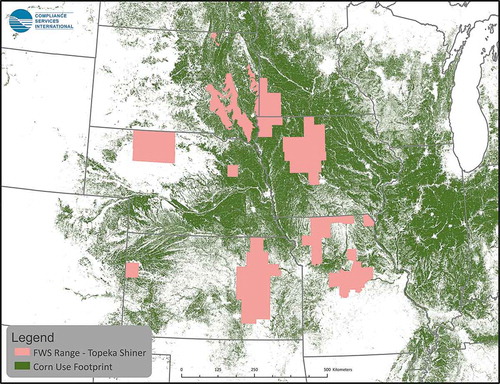
The USEPA (2009b) evaluated the potential direct and indirect effects of atrazine on the federally threatened California red-legged frog (Rana aurora draytonii) and the delta smelt (Hypomesus transpacificus). In addition, this assessment evaluated whether labeled use of atrazine was expected to result in modification of designated critical habitat for these two species. Screening level methods included use of standard models such as PRZM-EXAMS, T-REX, TerrPlant, and AgDRIFT. In addition, T-HERPS was used to refine estimates of exposure and risk to amphibians. The results of the assessment for the aquatic phase of the California red-legged frog (eggs, larvae, and adults) indicated no acute or chronic LOCs were exceeded for aquatic phase amphibians based on available fish and amphibian data (USEPA 2009b). However, the designation of LAA was applied to aquatic phases of the California red-legged frog by virtue of adverse effects on prey and modification of critical habitat. A similar designation was applied to the terrestrial phase of the frog (USEPA 2009b). Similarly, no exceedances of LOCs for Delta smelt were identified but, a designation of LLA was assigned because of indirect effects on habitat and food source (USEPA 2009b).

5.2.2 Weight of evidence and the effects on and risks of atrazine to aquatic vertebrates

Starting around 2000 and continuing until today, there have been many studies conducted which have examined the effects of atrazine on aquatic vertebrates, notably fish and amphibians. Some of these studies were highly publicized in that they made claims that atrazine at low, environmentally relevant, concentrations had the potential to negatively impact growth and development in amphibians, which reflect apical responses critical to ecological risk assessment. This spurred considerable activity within the USEPA and the broader community in understanding potential risks posed by atrazine. There was concern that many of the responses being considered, such as aspects of sexual differentiation, and laryngeal development, were not commonly used in risk assessment. Moreover, there was an increased emphasis on the measurement of responses at the cellular and molecular levels of organization and how these should be integrated in risk assessment was unclear. There was a secondary issue that required consideration and that related to the characterization of environmental exposures owing in part to changes in the application rates being employed for atrazine use. All these features play into the questions of how to assess listed species.

The USEPA has evaluated the potential impact of atrazine on frogs and other amphibians for more than 15 years. Since 2003, the Agency has written numerous white papers, held three FIFRA Scientific Advisory Panels (SAPs) (USEPA 2003c, 2007g, 2012c), required registrants to conduct extensive studies, and exhaustively evaluated all relevant peer-reviewed literature (USEPA 2012c). Several studies published in the early 2000s (e.g., Hayes et al. 2002a, 2002b, 2003, etc.) were considered by the Agency, which concluded that “ … none of the studies fully accounted for environmental and animal husbandry factors capable of influencing endpoints that the studies were attempting to measure … ” (USEPA 2003c). Consequently, as recommended by the 2003 SAP and under the Agency’s direction and supervision, the primary registrant, Syngenta, conducted a definitive amphibian study in 2006/2007 (Kloas et al. 2009). The Agency subsequently concluded in 2007 that “In laboratory studies where environmental and animal husbandry factors were controlled, atrazine exposures (0.01–100 μg/L) did not affect time to or size at metamorphosis, sex ratio, or gonadal development” (USEPA 2007g). This study contributed to the development of the amphibian metamorphoses assay (AMA), as part of the Agency’s endocrine disruption screening program (EDSP). Furthermore, in preparation for the 2012 SAP, the USEPA conducted another comprehensive review and concluded that “EPA does not have additional data on amphibians that is sufficient and robust which alters its quantitative understanding of the potential toxicity of atrazine to this taxon” (USEPA 2012c). However, the 2012 SAP recommended EPA conduct a rigorous weight of evidence analysis that incorporated study quality concerns without overreliance on a single study (USEPA 2012e) resulting in subsequent deference to qualitative approaches (USEPA 2016) rather than systematic quantitative weight of evidence (QWoE) analyses predicated on study quality, relevance, or consistency. Two, published QWoE analyses (Hanson et al. 2019b; Van Der Kraak et al. 2014) applying numerical scores to weigh study strength and relevance to apical endpoints have concluded that there was a lack of compelling evidence for adverse effects of atrazine on fish, amphibians, or reptiles at acute and chronic exposures below 100 µg/L.

To date, well over 200 publications in journals and technical reports have described the direct effects of atrazine exposure on aquatic vertebrates. Making sense of these data has been complicated by the variety of methods employed, the diversity of the species examined and large variations in the concentrations of atrazine tested. In an effort to interpret these data, a quantitative weight of evidence (QWoE) approach was proposed and used to evaluate all of the available data and to establish a consistent, transparent, and defensible set of criteria to evaluate the quality of the methods of the studies and the relevance of the results to apical endpoints (Van Der Kraak et al. 2014). The apical endpoints were survival, growth, development, and reproduction and the assessment of each study followed consistent guidelines and was verified by independent quality assurance. This QWoE was updated to include additional studies up to 2019 (Hanson et al. 2019b), which followed the same framework for assessment. No studies were omitted based on quality, so the process was inclusive and was transparently reported. Together, these QWoEs evaluated 1611 responses in more than 75 species of fish, amphibians, and reptiles.

In conducting this QWoEs analysis, it was necessary to define what would be considered as an ecologically relevant atrazine concentration. It was established that, if the LOEC for a toxicity test was ≥100 µg/L for an exposure period ≥96 h, the response was deemed to occur at an environmentally unrealistic concentration and the result was not considered as being relevant. The cutoff value of 100 µg/L was based on four-day rolling averages determined from measurements in vulnerable watersheds in the USA (see Table 2 in Van Der Kraak et al. 2014). Combining the two probabilities (0.8 and 0.99) discussed in characterization of the AEMP in Section 3.3.3.1 indicates that the value of 53 µg/L represents the 99.8th centile of expected daily concentrations across the USA.

Table 6 summarizes the QWoE analysis of the effects of atrazine on apical responses related to the survival, growth, reproduction, and development in fish, amphibians, and reptiles. The analysis was based on scores from 0 to 4 for both relevance of the response and the quality of the methods. If the mean score for relevance was zero, the null hypothesis of causality (that atrazine, at concentrations commonly found in the environment, does not cause effect “x”) was clearly considered not falsified. When the score for relevance was 3 or greater, the null hypothesis was considered falsified. Consistently the data for the apical endpoints scored less than 0.2 which a strong demonstration that atrazine at environmentally relevant concentrations, is unlikely to have ecologically significant effects in fish, amphibians, or reptiles. The experimental design, appropriateness of the hypotheses, and quality of methods (QoM) were also scored from 0 to 4. A score of 0 was assigned if the design and methods were very weak and a score of 4 assigned if it there were no weaknesses. These scoring approaches were similar to those recommended by the USEPA for assessing studies from the open literature (USEPA 2011; USEPA 2012a).

The weight of evidence assessment (Table 6) showed a lack of sensitivity of apical endpoints (development, survival, growth, and reproduction) for aquatic vertebrates. However, the chronic fish endpoint selected by USEPA in the 2016 ecological risk assessment of atrazine (USEPA 2016) was based on a study with Japanese medaka; Oryzias latipes) (Papoulias et al. 2014) that had several major weaknesses (pointed out in the QWoE analysis Van Der Kraak et al. 2014). Similarly, an earlier study on fathead minnow (Tillitt et al. 2010) suffered from several weaknesses also discussed in (Van Der Kraak et al. 2014). These two studies were not used in the 2020 draft BE (USEPA 2020b). From the responses to atrazine evaluated in the QWoE (Table 7), the most appropriate conservative criterion is the NOAEC of 65 µg atrazine/L from Macek et al. (1976).

The USEPA selected sublethal and chronic responses for fish in its BE (Table 2–4 and 4–1 in USEPA 2020b) that were based on a study by Nieves-Puigdoller, Björnsson, and McCormick (2007) in Atlantic salmon (Salmo salar) exposed to nominal concentration of 10 and 100 µg atrazine/L for 21 days in fresh water (not 30 days as reported in the BE). The responses used by EPA were decreases in food intake, length, weight, and growth rate, which are all correlated to food intake. These decreases were observed at 100 µg/L only and there was recovery after transfer to sea water for 90 days. The Nieves-Puigdoller et al. study had a number of weaknesses (as evaluated in QWoE assessment by Van Der Kraak et al. 2014) and the effects on weight could not be replicated in a stronger study on the same species with more replicates and fish per replicate. (Matsumoto, Hosmer, and Van Der Kraak 2010). Also, in its draft 2020 BE, EPA selected the most sensitive sublethal effect for aquatic stages of amphibians from a study on larvae of Xenopus laevis exposed to atrazine for 90 days (not 30 days as indicated in Table 2–4 in USEPA 2020b). The only two significant responses were decreased weight of liver and testes in frogs exposed to the highest nominal concentration of 100 µg atrazine/L (Sai et al. 2016). This study also had a number of weaknesses (including sourcing the eggs from only one female, lack of a water-only control, use of DMSO as a solvent, infrequent measures of exposure concentrations, and lack of information on water-quality and husbandry) and the results were inconsistent with other studies in the same and other species of frogs (as evaluated in QWoE assessments by Hanson et al. 2019b; Van Der Kraak et al. 2014). Both of these responses are poorly supported lines of evidence that are incongruous with apical effects and other responses in the QWoE assessments.

Overall, the results of QWoE assessments did not identify any adverse direct effects of atrazine on fish and amphibians at concentrations less than 100 µg atrazine/L. There were fewer studies on reptiles, but these did not indicate adverse direct effects either. Lack of relevant effects observed in reptiles is not unexpected given that the pathway of exposure for reptiles is almost totally through residues in dietary items and would be small or incomplete because of lack of bioconcentration and biomagnification of atrazine.

5.2.3 Observed indirect effects on aquatic vertebrates

While the studies discussed above demonstrate that atrazine is not directly harmful to fish and amphibians at environmentally relevant concentrations, it has the potential to negatively impact these species through indirect effects on non-target aquatic plants and invertebrates in areas where there are significant exposures. Investigations of these indirect effects are often conducted in cosms where there is the opportunity to control the species distribution and abundance in order to distinguish the interactions. Indirect effects on aquatic invertebrates have also been studied in cosms.

In the Kansas cosm studies (DeNoyelles et al. 1989; DeNoyelles, Kettle, and Sinn 1982), as described in Section 4.3.2 above, some atrazine treatments (in combination with receding water levels and overgrazing by grass carp) resulted in severe reductions in macrophyte biomass, which, in some cases, resulted in indirect effects on aquatic insects (Dewey 1986) and other aquatic macrophytes (Huggins, Johnson, and deNoyelles 1994), and also caused reductions in bluegill sunfish populations due to loss of macroinvertebrate food supply and loss of cover for juvenile fish (Kettle et al. 1987). In a study using cosms similar to the Kansas ponds, Fairchild, La Point, and Schwartz (1994) observed less severe effects on macrophytes (shifts in species composition without a reduction in total biomass or productivity) at 50 µg/L atrazine, with no indirect effects on zooplankton or fish. In one of the Kansas studies (DeNoyelles, Kettle, and Sinn 1982), the dominant zooplankton species was reduced in ponds treated with 500 µg/L atrazine, an effect attributed to reductions in abundance of phytoplankton; no significant effects on zooplankton were observed in other studies at the Kansas site.

Diana et al. (2000) measured the length and weight of larval gray tree frogs (Hyla versicolor) in 90-L outdoor pools treated with 20, 200, and 2000 µg/L atrazine. As discussed in Section 4.3.2.2 above, concentrations of dissolved oxygen decreased immediately in the cosms treated with 200 and 2000 µg/L. At these concentrations, frogs were 5% shorter and had 10% lower body mass at metamorphosis than in controls and 20 µg/L. The authors suggested that the effects on frogs may have been due to the declines in dissolved oxygen caused by elimination of macrophytes at these higher concentrations.

Rohr et al. (2008b) hypothesized that the direct effects of atrazine on phytoplankton and macrophytes could generate a cascade of indirect effects. Reduced growth of phytoplankton or macrophytes could increase availability of nutrients and light for periphyton, which could result in an increase in periphyton. As a result, numbers of trematodes that use snails as intermediate hosts could increase in response to the increase in populations of snails; and amphibians could be affected by the increase in trematode infections. This hypothesis was based in part on a cosm study rated low for both relevance and quality (Giddings et al. 2018). The same hypothesis was tested in a high-quality cosm study by Baxter et al. (2011), who observed a reduction in macrophyte biomass at 100 µg/L atrazine (approximately the same concentration tested by Rohr et al. 2008b) but no accompanying increase in snail density suggesting no cascading effects on frogs via infections with parasitic trematodes.

Overall, the cosm data support the conclusion that effects of atrazine on aquatic plant communities can, under some circumstances, result in indirect effects on other components of aquatic ecosystems. However, such indirect effects require substantial impacts on the plant community. The high-quality cosm studies reviewed above reported relatively minor indirect effects even at concentrations of ≥200 µg atrazine/L for significant durations of time, concentrations that cause severe effects on plants but are in any case unlikely to occur in the field. We conclude that the risk of indirect effects of atrazine to listed aquatic animal species mediated through direct effects on aquatic plants is negligible. This empirically based conclusion is consistent with population modeling results described in Section 4.4 above.

5.2.4 Recent advances in modeling indirect effects on aquatic vertebrates

Listed species are not available for direct field collection or laboratory studies, thus consideration of the potential effects of pesticides relies on the development and application of innovative ecological modeling approaches. One such modeling approach was used to examine the potential effects of atrazine exposure on the ecological production dynamics of species of aquatic plants, invertebrates, and fish in a generalized Iowa headwater pool and the consequences for Topeka shiner (Notropis topeka) populations (Bartell et al. 2019). The Topeka shiner is a small, endangered minnow that inhabits the upper Great Plains of the USA and its species-range overlaps areas of atrazine use (Figure 23). This analysis included hybrid modeling, an integration of an individual-based model and a food web-ecosystem model (CASM_TS), which provided a food web–ecosystem context to assess the impacts of exposure to atrazine. The CASM_TS, informed by previous Midwestern stream modeling, includes multiple representative populations of aquatic plants and consumers, which represent prey items for Topeka shiners in the individual-based model.

Risks posed by atrazine runoff were assessed for worse-case exposure scenarios based on within-stream monitoring data for selected locations in Nebraska, Missouri, and Iowa that are highly vulnerable to runoff. To further examine the utility of the hybrid model in assessing potential atrazine risks, toxic effects were also simulated for hypothetical exposure scenarios. In the simulation, concentrations were systematically increased by multiplying daily values of the Midwestern monitored exposure concentrations by factors of 2, 4, and 5. Hypothetical scenarios also included constant daily exposure to atrazine at concentrations of 10, 50, 100, or 250 µg/L. The range of exposures was tested to examine the ability of the consequences of these effects on biomass of populations of Topeka shiners. Only indirect effects, via the food web, were evaluated on shiner populations in this study.

The results of the hybrid model suggest that, compared with baseline conditions, atrazine at concentrations reported for representative midwestern streams and for scenarios whereby these concentrations were multiplied by 2, 4, or 5 and for a constant exposure to 10 µg/L had minimal impacts on the biomass organisms that are preyed upon by Topeka shiner. Effects were characterized as differences between values for population biomass of 365‐d baseline and exposure simulations. The results indicated no discernable food web effects for monitored atrazine concentrations or constant exposures of 10 µg/L on Topeka shiner populations for either exposure scenario. Magnified monitored concentrations and higher constant concentrations produced greater modeled indirect effects on Topeka shiners. The results for the constant daily exposures of 250 µg/L in the hybrid model demonstrated the ability of the model to simulate reductions in Topeka shiner biomass when it was assumed that the plant community was composed mainly of sensitive plants. The reductions result from the negative impacts of these exposures on zooplankton. The increased macroinvertebrate biomass obtained for these exposures contributed to increased Topeka shiner population biomass during the fall months. In contrast, the hybrid model using less tolerant algal toxicity benchmarks essentially eliminated biomass of detritus, zooplankton, periphyton, and macroinvertebrates and correspondingly predicted reduced Topeka shiner biomass to 0 by July or September for the constant daily exposure of 100‐ and 250‐µg atrazine/L. The results of this hybrid modeling approach to risk assessment extend the previous assessments of atrazine that focused on alterations in periphyton community structure (Bartell et al. 2013; Nair, Bartell, and Brain 2015). The hybrid model emphasized the potential impacts of atrazine on zooplankton and macroinvertebrates, important prey for the Topeka shiner and predicted no adverse effects on the Topeka shiner at environmentally realistic exposures.

5.3 Effects on aquatic invertebrates

5.3.1.Early assessment of effects on and risks to listed aquatic invertebrate species

Similar to what was done for aquatic vertebrates, USEPA (2007d) conducted assessments that considered the potential direct and indirect effects of the herbicide atrazine on the survival, growth, and reproduction of eight Federally listed species of freshwater mussels: pink mucket pearly mussel (Lampsilis abrupta), rough pigtoe mussel (Pleurobema plenum), shiny pigtoe pearly mussel (Fusconaia edgariana), fine-rayed pigtoe mussel (F. cuneolus), heavy pigtoe mussel (P. taitianum), ovate clubshell mussel (P. perovatum), southern clubshell mussel (P. decisum), stirrup shell mussel (Quadrula stapes), fat pocketbook pearly mussel (Potamilus capax), purple cat’s paw pearly mussel (Epioblasma obliquata obliquata), and the northern riffleshell (Epioblasma torulosa rangiana). These assessments parallel what was done for vertebrates in terms of direct effects on growth reproduction and survival. The assessment of indirect effects is more complicated. This includes indirect effects related to mussel individuals via

• Reduction in food items (i.e., freshwater phytoplankton and zooplankton).

• Reduction in host fish for the glochidia stage of mussels.

• Direct effects to aquatic plants (i.e., reduction of habitat and/or primary productivity).

• Reduction of terrestrial and emergent vegetation (i.e., riparian habitat) required to maintain acceptable water quality and habitat.

In addition, this assessment evaluates the potential for atrazine use to result in the destruction or adverse modification of designated critical habitat for the ovate clubshell and southern clubshell mussels (the only two of the eight listed species for which critical habitat has been designated by the U.S. Fish and Wildlife Service). This assessment was completed in accordance with the U.S. Fish and Wildlife Service (USFWS) and National Marine Fisheries Service (NMFS) Endangered Species Consultation Handbook (USFWS & NWFS 1998) and procedures outlined in the Agency’s Overview Document (FWS & NOAA 2004).

These assessments suggested no direct acute effects whereas the assessment for chronic direct effects was MA, but NLAA. In terms of effects on plankton there was concern that atrazine may affect but was not likely to affect. As zooplankton are not a direct food source for mussels this may be of limited concern. In terms of effects on host fish species there was no evidence of acute direct effects although, for chronic responses, there was some concern as chronic LOCs are exceeded. Even at that, the interpretation was that chronic exposure was not likely to result in “take” of a single mussel via direct effects to host fish in vulnerable watersheds. In terms of indirect effects on either aquatic plants or riparian vegetation there was concern that these may be affected because terrestrial plant RQs are above LOCs. The MA and NLAA determination for listed mussels that are near grassy/herbaceous riparian areas was based on the sensitivity of aquatic plants and herbaceous vegetation to atrazine.

Other studies considered possible effects of atrazine on the dwarf wedgemussel (Alasmidonta heterodon) in the Chesapeake Bay Watershed (USEPA 2006a). There was no evidence of a direct effect of atrazine on this species or of an indirect effect via a reduction of aquatic animals as a food supply. In terms of indirect effects, it was concluded that atrazine exposure was not likely to have an adverse effect by a reduction of aquatic plants as food items or primary productivity or via direct effects on riparian areas required to maintain acceptable water quality and spawning habitat. In part, this was because there is no known obligate relationship between the assessed species and any single aquatic plant species, and short-term and long-term concentrations of atrazine were estimated to be lower than established thresholds for community-level effects to aquatic vegetation.

5.3.2 Direct effects of atrazine on aquatic invertebrates

Compared to vertebrates there are less data available in terms of the possible effects of atrazine on invertebrates. However, the available data indicate invertebrates in general are not highly sensitive to atrazine.

The fifth centile for acute (48–96-h) toxicity in aquatic arthropods was estimated to be 130 µg/L from data in Giddings et al. (2005), when compared to the appropriate 4-d rolling average concentration for atrazine from the AEMP program was greater than the 99th centile concentration of 24 µg/L (see Section 3.3.3 above), suggesting de minimis risk from acute exposures.

There is a paucity of information on the toxicity of atrazine and many other chemicals to mollusks and clams (bivalves) in general. Several studies have assessed effects on mollusks. Based on laboratory toxicity tests with the freshwater snail Biomphalaria alexandrina, the 24-h LC10, 50, and 90 were reported as 330, 1250, and 4750 µg/L, respectively (Barky et al. 2012). Longer exposures (4 weeks) at 330 µg/L resulted in mortality (55% at 4 weeks) reductions in number of eggs laid, hatchability, and increases in number of abnormal eggs. Several physiological parameters were also affected at this concentration. This paper had several weaknesses, such as lack of verification of exposures, lack of clear description of the toxicity tests and parameters of the water quality in these tests; however, the LC10 was much greater than the upper centile concentrations measured in the AEMP (see Section 3.3.3 above). In a guideline study on Eastern oyster (Crassostrea virginica), using shell-deposition as a test endpoint, the EC50 was >17,000 µg/L (Syngenta 2005).

A few studies characterized in a quantitative weight of evidence assessment (Van Der Kraak et al. 2014) included mollusks in relation to their role in transmission of trematode parasites. Survival of snails (Planorbella trivolvis) and number of egg masses deposited in cosms treated with atrazine at 201 µg/L (Rohr et al. 2008a) and survival at 50 µg/L (Rohr and Crumrine 2005) was unaffected; however, mass of snails and number of egg masses were reduced at this concentration. In another study, the number of eggs and the number of those that hatched was reported to be increased in the same species of snail in cosms treated with 117 µg/L (Rohr et al. 2008b). The number of snails (Physella spp and Stagnicola elodes), mass of snails, number of egg-masses, and number of eggs per egg-mass were all unaffected in cosms treated with atrazine at concentrations of 1, 10, 30, and 100 µg/L (Baxter et al. 2011). No effects on survival of Physa acuta exposed to atrazine in the laboratory were observed at 3 and 30 µg/L for 28 days (Gustafson, Belden, and Bolek 2016). This study was assessed in the update of the QWOE (Hanson et al. 2019a) and, despite equivocal results in some papers from the same laboratory, these studies do not indicate that atrazine has direct effects on fresh-water mollusks at environmentally realistic concentrations.

Only five studies on the effects of atrazine on bivalves (clams) were found in the literature. In a well-reported study on the effects of technical atrazine on juvenile Mercenaria mercenaria, Lawton et al. (2006) reported a 96-h LC50 of 5608 µg atrazine/L (95% CI; 5003–6287 µg/L). In 10-d exposures, NOECs and LOECs for survival and sublethal effects on shell-deposition and several other growth parameters were reported as 500 and 1000 µg/L, respectively. A toxicity test in sediment at concentrations up to 20,000 µg atrazine/kg showed no effects after 10 days of exposure.

In assays of the effects of a commercial formulation of atrazine (Atrazine 4 L) on glochidia of the freshwater mussel, Utterbackia imbecillis the 24-h LC50 based on nominal concentrations was 241,300 (SD = 48,800) µg/L (Conners and Black 2004). Comet assays for genotoxicity were attempted but the gels were damaged, and results could not be quantified. The study had several limitations in that exposures were not verified and that raw data for the responses in the toxicity test were not provided. The LC50 value for atrazine greatly exceeded the maximum solubility in water (33 mg/L); however, taken at face value, the results do not indicate high toxicity to glochidia and are consistent with the reported LC50 of >60,000 µg atrazine/L in glochidia of the same species Utterbackia [Anodonta] imbecillis (Johnson, Keller, and Zam 1993) as listed in (Bringolf et al. 2007) but not cited.

The toxicity of technical atrazine was reported in a well-reported study on glochidia and juvenile stages from freshwater mussels collected from rivers and streams in generally forested, rural areas of North Carolina and Missouri, USA. The species were Elliptio complananta, Lampsilis fasciola, Villosa constricta, V. delumbis, Lampsilis siliquoidea, and L. fasciola (Bringolf et al. 2007). The 24- and 48-h LC50s for glochidia of all species were >30,000 µg atrazine/L (the authors did not test at concentrations > maximum solubility of atrazine in water). In addition, the 48-h LC50s for juveniles of L. siliquoidea, and L. fasciola were also >30,000 µg/L. Chronic (21-day) assays on growth of juveniles of L. siliquoidea showed significant reductions in growth rate at 3750 µg/L but not at 1900 µg/L. These results do not indicate significant adverse effects at environmentally realistic concentrations. In a paper published in Thai (Nuchan et al. 2018) the English abstract states that the 96 h LC50 in adults of the freshwater pearl mussel, Hyriopsis bialata was 158,000 µg/L. No further details were available, so the quality of the test could not be assessed. Overall, acute, and chronic toxicity tests conducted in the laboratory indicate very low sensitivity of freshwater mussels to the direct effects of atrazine. While some clams have an obligate relationship with fish in terms of early development of the glochidia, specificity of host fish varies considerably among freshwater mussels, from obligate to lower fidelity (e.g., generalists) (INHS 2020), However, the limited sensitivity of both the glochidia and fish hosts to atrazine (Section 5.2.2) suggest that this stage of development is not susceptible to atrazine.

5.3.3 Indirect effects on aquatic invertebrates

Indirect effects of exposure of aquatic invertebrates to atrazine have been studied in cosms. As for vertebrates, cosm studies offer the best methods for characterizing indirect effects of exposures to atrazine. Cosm studies on community response to atrazine are usually conducted with chronic exposures. These chronic exposures to constant or slowly declining concentrations present a worst-case when compared to more realistic exposures in the field that vary over time (see Section 3.3.3 above). Specifically, they do not allow consideration of recovery of photosynthesis from temporary stasis.

Hamilton et al. (1989) observed temporary reductions in some species of rotifers, cladocerans, and copepods in lake enclosures treated with 155 µg/L atrazine, effects that were attributed to changes in quality of phytoplankton food. The indirect effects were small; total rotifers, total cladocerans, and total copepods were not significantly reduced. As discussed above (Section 5.2.3 above), Rohr et al. (2008b) hypothesized that the direct effects of atrazine on phytoplankton and macrophytes could generate a cascade of indirect effects resulting in an increase in periphyton which could increase populations of snails. This cosm study was assessed to be of low quality and relevance (Giddings et al. 2018) and, when tested in a high-quality cosm study by Baxter et al. (2011), there were no effects on density of snails despite a reduction in biomass of macrophytes at 100 µg/L atrazine.

Although there is paucity of studies on the indirect effects of atrazine on invertebrates in cosms, such indirect effects would require substantial impacts to the plant community. High-quality cosm studies (see Section 4.3.2 above) reported relatively minor indirect effects, even at atrazine concentrations of ≥200 µg/L for significant durations of time and concentrations that cause severe effects on plants. These concentrations and durations are unlikely to occur in the field. We conclude that the risk of indirect effects of atrazine to listed aquatic animal species mediated through direct effects on aquatic plants is negligible. This empirically based conclusion is consistent with population modeling results described in Section 5.2.4 above.

As clams are filter feeders, it is possible that they could be indirectly affected by effects on food supply, either via phytoplankton or detritus from plants in riparian areas. Specific studies on indirect effects of atrazine on clams were not found in the literature but a risk assessment of the potential indirect effects of atrazine on the listed species; fat pocketbook pearly mussel (Potamilus capax), purple cat’s paw pearly mussel (Epioblasma obliquata obliquata [PPCP mussel]), and the northern riffleshell (Epioblasma torulosa rangiana) was conducted by the USEPA (USEPA 2007f). This assessment predated more recent guidelines for listed species but did include data from the early measurements in the AEMP and data on flowrate in preferred habitats. From simple Tier-1 assumptions, the assessment concluded that these species would be LAA by atrazine via availability of “prey” and effects on habitat. But, on more detailed analysis the report states that:

“However, atrazine is not likely to adversely affect the fat pocketbook mussel in watersheds with predominantly forested riparian areas because woody shrubs and trees are generally not sensitive to environmentally relevant concentrations of atrazine. In addition, atrazine-related impacts to riparian areas adjacent to large rivers occupied by the fat pocketbook are expected to be insignificant, based on a spatial analysis of land cover data adjacent to occupied rivers. Potential indirect effects to the PCPP mussel and northern riffleshell via atrazine-related impacts to riparian vegetation adjacent to the occupied streams/rivers are also not expected, based on an analysis of land cover and county-level use data, as well as aerial satellite photography. Therefore, the effects determination for the fat pocketbook mussel located in watersheds with predominantly forested vegetation (including big rivers), and for the PCPP mussel and northern riffleshell in all occupied watersheds is NLAA.”

This is a good illustration of how a Step-2 assessment should be carried out on listed species. Aerial observation is possible with several sources of imagery from satellites, such as Ikonos, drones, and aircraft fitted with cameras and multispectral sensors. Positional data from these sources allow action areas to be identified and proximity to species-ranges of listed species to be quantified at higher resolution.

5.4 Strengths and uncertainties

A strength in the assessment of the potential effects on listed species is the large literature base for aquatic vertebrates and invertebrates which provides a high degree of certainty in making conclusions of the risks posed by exposure to atrazine. The lack of data on aquatic invertebrates and their evolutionary divergence adds to the uncertainty in understanding how these species may be affected by atrazine. Understanding the possible indirect effects of atrazine, is an area where more work could be conducted. For future needs, modeling capabilities should be expanded and validated where possible. Like aquatic plants, we recommend a better understanding of similarities between listed and non-listed species in terms of their life-history and ecological traits.

6 Effects of atrazine on non-target terrestrial plants

6.1 Problem formulation

As an herbicide, atrazine could adversely affect non-target plants, via reduced growth rates or, should exposures be substantial and sustained, via changes in structure and function of plant communities that, if severe enough, could cause indirect adverse effects on other terrestrial organisms. These effects would be mediated via photosynthetic starvation in plants and/or the production of secondary toxic substances (Shimabukuro et al. 1971). Dicotyledonous plants are somewhat more sensitive than monocotyledonous plants, (Brain and Hoberg 2016; Dalton and Boutin 2010; White and Boutin 2007) but not to the extent that atrazine could be considered selective. In the laboratory and field, atrazine does not typically cause rapid mortality (e.g., the complete loss of all viability with no potential for recovery) in terrestrial or riparian plants at environmentally realistic exposures and durations (Brain et al. 2019; Brain and Hoberg 2016; Dos Santos et al. 2020; Wang et al. 2015; White and Boutin 2007) and, as discussed above (Section 2.4), plants can recover. Also noted in Section 2.2 above, there is no evidence of bioaccumulation of atrazine in terrestrial plants beyond general uptake as would be expected for an herbicide with its physicochemical properties that result in transport in the xylem with minimal systemic transport when applied to leaves. This means that concentrations in plant tissues would be expected to decline rapidly after exposure, allowing for recovery and reducing non-target exposure in herbivorous organisms. Experimentally, it has been shown that upon termination of exposure to atrazine the inhibition of growth ceases and recovery (e.g., a return to control level growth rates) is observed in both monocots and dicots within days (Brain and Hoberg 2016). As atrazine is typically applied once a year in most use-scenarios (see SI Section 2), there is a significant window for recovery to occur should there be any impairment of growth.

Should they occur, exposures of plants in off-field terrestrial and riparian habitats would be driven primarily by spray drift (typically resulting in foliar exposure) and run-off from the site of application following significant rainfall events or via sub-surface ground water flow through soil (resulting in root uptake and seed- or seedling-stage exposure, see Section 3.3.1 above). The life-stage of at which non-target plants could be exposed depends on the timing of application but, given the label uses at this time (see SI Section 2), the most likely scenario is that terrestrial plants will have germinated and be in a vegetative growth phase for annuals, with perennial plants well established. For spray drift, atrazine exposure would occur as formulated product, but via runoff (soil) exposure would occur as the active ingredient. For spray drift or runoff, exposures off-field are expected to be low (see Section 3.3.2 above).

Relevant to field runoff, 3-m wide vegetative filter strips have been found to attenuate movement of atrazine via runoff by up to 99% (Lafrance, Caron, and Bernard 2013). Atrazine is also typically applied only once a growing season, so cumulative exposures (and hence effects) are not likely to occur. Concentrations of atrazine in plant tissues from treated crops such as corn, which could move off field and contribute to soil as end of season plant residue are very low and consist mostly of the metabolite hydroxy atrazine. Li et al. (2019) reported the rapid uptake and metabolism of atrazine from soil by corn, meaning that transport to surrounding vegetation by silage or via soils is significantly reduced by the crop itself. Based on a survey of soils across the USA, Mueller et al. (2017) found the mean half-life in soils where atrazine was used regularly was 2.3 days (as opposed to 14 days where it was not used), meaning movement off-field is again likely to be limited to a great extent. Albright et al. (2013) found no detectable atrazine in switchgrass plants or soil at >14 days after treatment. Given that atrazine is relatively soluble in water, further dilution in soils over time via infiltration of water in addition to biodegradation would reduce exposures further. This means exposures to atrazine via soil containing residues are generally low (in the ng/kg range), limited to the cropped area, and highly unlikely to be a source of exposures in critical habitats for listed plants.

Currently (as of 2020) in the USA, there are many endangered terrestrial plants species and, correspondingly, a considerable geographic area ascribed to critical habitat. In the conterminous USA, there are currently ~445 listed terrestrial plant species (~186 in California), and 161 with a species-range located in counties which overlap >0.95% with areas where corn, sorghum, and sugarcane is grown (see SI Section 3, SI Table S3–5). As it is not possible to discuss all these plant species individually, several examples are provided below. Also, potential co-occurrence of species-ranges with rights of ways, forestry, and conservation reserve program (CRP) lands, as well as of the states of Hawaii, Alaska, and the U.S. territories (American Samoa, Guam, the Northern Mariana Islands, Puerto Rico, and the U.S. Virgin Islands) will not be exposed to atrazine; these uses/geographies are approved for off-labeling, and therefore exposures, should they have occurred in the past, will cease. Syngenta has no active registrations of atrazine in California.

Considering the lack of any significant off-field exposure, and the general lack of sensitivity by plants at concentrations found in off-field downwind drift with a protective buffer of 15 feet (4.6 m) or surface or sub-surface flow, it is unlikely that any currently listed endangered terrestrial plant species would be at a significant risk from the use of atrazine at approved label rates in the US. However, more accurate descriptions of the actual overlap between areas of corn production and species-range as discussed in Section 3.2.2 and SI Section 3 would illuminate any potential risks. Below we briefly summarize the available literature and laboratory and field studies as it relates to the possible risk posed to listed species.

6.2 Toxicity of atrazine to terrestrial plants

6.2.1 Laboratory studies in the effects of atrazine on plants

A recent review examining the relative sensitivity of crop and wild species of plants to herbicides determined there was no significant difference in their toxicological response (Christl et al. 2018). Therefore, there is no reason to believe that endangered plant species are inherently more sensitive than wild or crop species. Thus, data from crop and wild species could be used to predict potential responses and hence risk, of the former to any given herbicide. Another review also noted that vegetative and reproductive endpoints in terrestrial plants were similar in sensitivity to herbicides (Christl, Hoen, and Zumkier 2019). Overall, this indicates that crop species can be reasonably used as a surrogate for listed species, with the understanding that impairment of reproductive responses have greater implications for viability of populations of listed species. Taken together, vegetative responses for standard crop test species can be used to understand potential direct risks posed to endangered plants and for reproductive responses. These assumptions would apply to both laboratory and field-based studies for atrazine and are supported by the available data discussed below.

Brain and Hoberg (2016) reported the responses of ten species of plants (six dicotyledonous and four monocotyledonous) exposed to direct overhead application of a range of application rates of the same formulation of atrazine (Atrazine SC). After 14-d and 21-d, plants were assessed for seedling emergence and vegetative vigor, respectively. As discussed in Section 3.3.2 above, this study represents a worst-case spray-drift exposure scenario for non-target terrestrial plants. For seedling emergence, only 2 of 10 species tested, cabbage and tomato, exhibited strong concentration-responses. For vegetative vigor, 9 of the 10 species tested exhibited strong concentration-responses. Germination and emergence are highly conserved and often not sensitive to the herbicides and other chemicals unless they have a mode of action that that inhibits general metabolism or cell division. For photosynthetic inhibitors such as atrazine, vegetative vigor is a more appropriate endpoint for characterizing sensitivity. Because pre-recovery measures of effect for vegetative vigor used in the Brain and Hoberg (2016) study (shoot length, shoot dry weight, 21-day shoot length growth rate, and 21-day shoot dry weight growth rate) are all correlated, an SSD was constructed from the most sensitive endpoint, usually shoot dry weight (Figure 24).

Figure 24. Species sensitivity distribution of no observable effect spray concentrations constructed from data in (Brain and Hoberg 2016) for the most sensitive measure for vegetative vigor. Note that these data are from direct overhead spraying of the plants and are therefore not representative of exposure from downwind drift

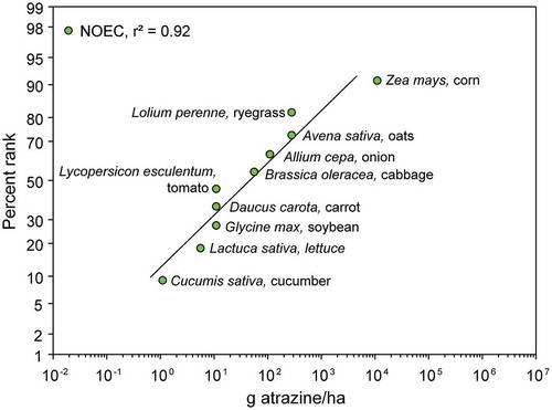
The most sensitive dicot tested in the vegetative vigor assay was cucumber (Cucumis sativa). Monocots were generally less sensitive and, as expected, corn was the least sensitive. In this study, Brain and Hoberg (2016) also characterized the potential for recovery of the ten tested species exposed to direct overhead application of atrazine (Atrazine SC formulation). Briefly, the vegetative vigor studies were extended by 21 days to allow for a recovery phase. Results from this study can be found in the SI for Brain and Hoberg (2016). They reported that, in most species where initial herbicidal effects were observed, the effects on rate of growth were largely ameliorated over time. Oat (Avena sativa), which was the most sensitive monocot tested in the emergence assays, exhibited full recovery at 28-d across all endpoints (NOECs ≥56 g a.i./ha nominal application rate), while growth rates in the dicot, cabbage (Brassica oleracea) showed substantial recovery with a NOEC of ≥280 g a.i./ha nominal application rate. Growth rates in onion (Allium cepa) recovered by 42-days with a NOEC of ≥280 g a.i./ha nominal application rate, while the dicot cucumber (C. sativa) growth rates showed full recovery with a NOEC of ≥280 g a.i./ha nominal application rate by the end of the recovery phase. These observations indicate that terrestrial plants can recover from unintentional exposures to atrazine, which further mitigates potential risks to listed and non-listed plants.

White and Boutin (2007) examined the biomass response of ten crop species and ten related wild species at 28-d following a one-time spray application of atrazine (AAtrex Liquid 480) at the two to six-leaf stage. They reported no significant difference in sensitivity to atrazine in cropped versus wild species for monocots versus dicots. For crop species where a 28-d biomass IC25 could be calculated, these ranged from 40 to 177 g a.i./ha (n = 8) and for wild species 20 to 2162 g a.i./ha (n = 9). In another study (Dalton and Boutin 2010) of single-species tests, nine non-crop terrestrial plants (perennials, biennials, monocots, and dicots) were treated with atrazine (AAtrex Liquid 480) via direct overspray. Of these nine, three were chosen for definitive testing, but no clear rationale was provided; however, it is a reasonable to assume that the three selected species were those that exhibited greater sensitivity. The three species included in the definitive assay, Alliaria petiolata, Geum canadense, and Symphyotrichum lateriflorum (all dicots) had reported 28-d biomass IC25s of >100 g atrazine a.i./ha. These observations in non-crop plants are consistent with those of White and Boutin (2007) and Brain and Hoberg (2016) and reaffirm other observations that wild plants are not more (or less) sensitive to atrazine.

Overall, in laboratory testing, there were no meaningful differences in sensitivity among various terrestrial plant taxonomic groups (e.g., monocots, dicots), life stage, or endpoint to atrazine across the available literature. Recovery following exposure to atrazine has also been consistently demonstrated across plant groups, life stage, and endpoints and should be considered in any assessment.

6.2.2 Field studies on the effects of atrazine on plants

The exposure of terrestrial plant communities to an herbicide can have adverse impacts on individual plant species, both directly via uptake and the manifestation of toxicity (e.g., failure to germinate, failure to set seed) regardless of the presence of other species, and indirectly, through changes in growth and reproduction patterns in species that are in competition (e.g., significant reduction in growth rate allowing other plants to outcompete each other; essentially what happens infield with many herbicides in relation to crops and weeds). As it pertains to atrazine, field- studies show no evidence of effects occurring at realistic exposures resulting from runoff and drift beyond 4.5 m (see Section 3.3.2 above and SI Section 4).

In a study on spray-drift, Brain et al. (2019) reported the response of cucumber and lettuce from exposure to spray drift deposition of AAtrex 4 L in the field. Exposing plants downwind to physical drift moving laterally away from the spray swath realistically reflects how non-target terrestrial plants would be exposed. Twenty-one days post-application survival, biomass, and shoot length were measured and contrasted with up-wind controls. Overall, the aggregate lowest observable effect distance (LOED) was 1.5 m from the end of the boom and the aggregate no observable effects distance (NOED) was 4.6 m (15 ft), with cucumbers affected more than lettuce which showed no adverse effects. Based on measured deposition of drift on horizontal collectors, deposition at the NOED was 10 g/ha (0.0079 lb./A. It is important to note that these were fully exposed plants (bare ground), with no surrounding vegetation for mitigation of exposure through interception, and windspeeds between 16 to 32 km/h (10 to 20 mph), representing a worst-case scenario for spray drift deposition (see Section 3.3.2 above and SI Section 4 for further information). Note that a maximum windspeed of 16 km/h (10 mph) for ground applications has been proposed voluntarily by Syngenta as a label mitigation.

Longer-term studies on field-plants sprayed with atrazine (AAtrex Liquid 480) showed that these plants were less sensitive than those tested in the greenhouse (Dalton and Boutin 2010). In addition to laboratory studies, the authors conducted more complex and longer-term model community experiments with eight non-crop species with testing in the greenhouse and outdoors (i.e., a 28-d greenhouse study, a 70-d greenhouse study, and an outdoor microcosm study, duration unclear but assumed to be 28-d). For the greenhouse 28-d community study, the IC25 for biomass was >100 g a.i./ha and the 70-d community biomass IC25 was >400 g a.i./ha, indicating significant recovery. For the outdoor study, the 28-d community IC25 for biomass was >300 g a.i./ha, indicating further that environmentally realistic testing showed mitigation of the effects of atrazine relative to tests in greenhouses.

Another line of evidence characterizing direct or indirect effects on non-target plants at the population and community levels for both structure and function is the successful use of vegetative buffer strips to attenuate the off-field movement of atrazine, primarily via surface and sub-surface runoff. These buffers also present a highly effective and viable mitigation strategy for cropping in areas where movement off-field would be anticipated (see Section 8 below). Several studies have demonstrated the efficacy of these buffers to reduce movement of atrazine off-field, with no reported impacts on the buffer plant communities themselves. In a study in Missouri, USA, Lerch et al. (2017) reported that experimental 4-m wide vegetative buffers reduced off-field movement of atrazine by >60% for a variety of planting strategies, including native grasses. The efficacy of these systems was monitored for several seasons and years, with no impairment of the plant communities reported and with significantly improved soil quality relative to field control. In Quebec, Canada, Lafrance, Caron, and Bernard (2013) reported that 3-m wide simple grass buffer strips were typically effective at removing >90% of atrazine over a study period of several years, with no reported impairment of the plant communities themselves or reduced efficacy over time. In general, the continued functionality of buffer strips in agriculture through time and across landscapes is evidence of the lack of significant adverse effects of herbicides on near-field plant communities (Prosser et al. 2016).

6.3 Assessment of risks of atrazine to terrestrial plants under ESA

6.3.1 Direct effects

Herein we highlight several case studies for listed non-target terrestrial plant species and the potential for direct effects of atrazine. One of the major issues in assessing direct effects is the use of inappropriate test methods to characterize sensitivity of non-target plants to atrazine (and herbicides in general). In practice, non-target plants are not exposed via an overhead spray as would occur in the cropped area of the field; they are exposed to lateral, downwind drift (see Section 3.3.2 above). This downwind drift contains more small droplets and the effective volume of spray solution deposited on the plants is much less than a direct overspray. This likely reduces wetting of the leaves and may reduce efficacy of the chemical. The information for the effects of atrazine on off-field non-target plants indicates de minimis risks for adverse effects when good agricultural practice is followed, and appropriate downwind buffers are used (e.g., 15 ft or 4.6 m). With the inclusion of buffer strips as a mitigation measure on future labels (see Section 8), exposure to non-target plants via soil infiltration or runoff is further reduced, resulting in even less risk of an adverse effect.

6.3.2 Indirect effects

With the approved removal of atrazine from forestry uses, there are no locations where there are more than 0.95% overlaps between species-range and for obligate animal–plant relationships between any listed plants and listed herbivores. Therefore, indirect effects via these relationships are not relevant scenarios. There are listed vertebrate and invertebrate species that rely on terrestrial plants in general for food, habitat, and other resources but, since plant communities in general will likely not be adversely impacted by atrazine used in accordance with the proposed changes in labels, these non-obligate relationships will not be affected.

6.4 Modeling effects of atrazine in non-target terrestrial plants

Evaluation of exposure and effects on non-listed and listed species of terrestrial plants typically begins with TerrPlant⁴. This spreadsheet-based model provides screening-level assessments of exposure from single pesticide applications. Based on the estimated environmental concentrations (EECs) and provided effects endpoints, risk quotients (RQs) are calculated for dry and semi-aquatic, listed and non-listed, monocot and dicot species. For listed species, RQ calculations are based on no observed adverse effect concentration (NOAEC), whereas EC25 is used for non-listed species.¹¹

There are several population models of terrestrial plants, including threatened and endangered, which integrate species-specific life-history traits as well as their ecological interactions and realistic exposure profiles for a more comprehensive risk assessment. For example, a matrix model of the threatened Mead’s milkweed (Asclepias meadii) was applied to assess impacts of two herbicides, including atrazine (Schmolke et al. 2018b). Model code and input files for this study are provided as supplemental material with the publication (Schmolke et al. 2018b). In a matrix model, the population is characterized by a certain number of stages or sizes. Individuals within one stage or size are assumed to be identical and transition to the next stage based on their survival, growth, and reproduction rates. The original Mead’s milkweed matrix model includes information on demographic data from 15 years of experimental planting at restored prairie sites in Illinois and Indiana (Bowles, McBride, and Bell 2015). The milkweed life cycle was represented with five life stages–a seedling, three non-flowering, and a flowering stage. Modeled exposure was based on spray drift and an exposure gradient was assumed and based on empirical drift-deposition curve data (see Section 3.3.2 above). Calculations were based on maximum application rates for both herbicides, as defined on the label. Only effects on vegetative vigor were included (Christl, Hoen, and Zumkier 2019) and were based on dose-response curves from guideline studies on cucumber, lettuce, soybean, and tomato. These were translated into effects on survival and as inhibition of growth that targeted different life stages in the model. The model ultimately translated individual-level impacts–growth and survival–to impacts on populations of Mead’s milkweed, specifically its population size. This was conducted in unison with altering burn sequences, as there were population data available for both burnt and non-burnt plots (Bowles, McBride, and Bell 2015). Multiple scenarios, also including exposure reductions using buffers, were simulated which identified that most population-level effects on this listed species can be mitigated with 4-m buffers.

Another modeling approach is the individual-based model (IBM) that was developed to assess risks from atrazine exposure to populations of the decurrent false aster (Boltonia decurrens) (Schmolke et al. 2017). Model code and input files for this study are provided as supplemental material with the publication (Schmolke et al. 2017). An IBM model represents a population as a collection of individuals that interact among themselves and with their environment. These individuals can differ by age, size, or any other property or trait that is modeled. As IBMs do not adhere to any mathematical formulation, they are more flexible than other approaches and can include life history, behavior, movement, and ecological interactions as well (Grimm and Railsback 2005). The decurrent false aster is a short-lived, herbaceous species and is listed as threatened throughout its range. As it depends on flooding for persistence of its populations, it is vulnerable to any flood control activities in its habitats which include the flood plains of the Illinois River. Its life cycle has two main pathways: starting with seedlings establishing in spring, developing into rosettes, and flowering in autumn. However, some plants can develop vegetative rosettes around flowering plants and can mature as unconnected plants in the following year. This IBM includes information on the species life cycle and simulates individual plants in a spatially explicit environment, where they experience intra- and inter-specific competition. Due to the dependence of the species on flooding, several flooding scenarios were simulated. Exposure to atrazine was simulated as spray drift exposure with the assumption that exposure at the edge of the field is greatest and then declines, following an empirical drift deposition curve (see Section 3.3.2). Exposure was translated to effects on survival and growth using treatment–response relationships based on carrot, cucumber, lettuce, soybean, and tomato vegetative vigor tests. Effects at the organismal level varied; the rate of deposition causing a 50% reduction in relative rate of growth (EC50_RGR in the paper), for example, ranged from 124 g/ha and 974 g/ha. The simulated effects at the population level; however, varied much less and were more driven by flooding conditions. This study demonstrated the need for relevant environmental factors and dependencies to be considered when assessing risks from exposure of listed species to atrazine.

The IBM for decurrent false aster was applied to simulate exposure from spray drift and runoff of the three herbicides–atrazine, mesotrione, and s-metolachlor–and its effects on population densities of this threatened species (Schmolke et al. 2018a). Different exposure pathways for the three herbicides were simulated separately and in combination. Effects data were based on seedling emergence and vegetative vigor studies which include testing impacts of herbicides on seedling emergence, seedling survival, and growth. When exposure to both runoff and spray drift co-occurred in simulations, effects were assumed to be additive. Finally, the model was applied to evaluate the efficacy of hypothetical setback distances to mitigate any potential adverse effects on this species. Exposure to runoff-impacted seedling survival and growth, and exposure to spray drift affected survival and growth of established plants. None of these organismal-level impacts correlated well with those at the population level, namely population density. This study also showed there were almost no predicted effects on any of the plant properties modeled with a spray setback distance of 4 m.

Given that in the conterminous USA there are currently 161 listed terrestrial plant species with a species-range located in counties which overlap more than 1% with counties corn, sorghum, and sugarcane (see SI Section 3, SI Table S3–1), it would be impractical to develop population models for each species. Moreover, the paucity of demographic and ecological data for most of these species presents challenges to the development of models. One possible avenue for addressing these data-gaps is the so-called “Robin Hood” approach (Punt, Smith, and Smith 2011). It proposes that assessments of data-rich species may inform assessments of data-poor species. However, the extent to which data-rich species are representative of data-poor species first needs to be determined. Whenever possible, comparative analysis of demographic data between listed and non-listed species should be conducted. An analysis of demographic traits of terrestrial plants, which included species within and outside of the USA, showed that individual traits such as net reproductive rate and generation time did not differ in species based on their status (listed vs. non-listed) (Rueda-Cediel et al. 2019). These traits were derived from plant matrix models which are populated with growth, survival, and fertility rates, which are derived from empirical data. This demographic analysis further revealed that, across listed and non-listed species, survival rates had the largest impact on population growth rates, followed by growth and, finally, fertility. These results imply that reliable knowledge of survival rates, or different factors contributing to survival, are highly relevant in assessing risks to populations of listed species. More importantly, this analysis strongly suggests that information from studies in non-listed, relatively data-rich terrestrial plants can be extrapolated to listed species with less data. The next step to explore is how species can be grouped based on limited availability of demographic, eco-physiological, and other data. This may lead to grouping listed species into plant functional types (Lavorel et al. 2007; Noble and Gitay 1996) or different trait-based clusters which may facilitate identifying representative species, data gathering, and model validation.

Overall, the population modeling that was applied to assess risks to listed species strongly suggests that environmental factors, such as flooding, and interspecific interactions are highly important in how species respond to exposure to herbicides, including atrazine. Under realistic conditions, impacts on the edge of the field population density of decurrent false aster did not exceed 9%-13%, for the duration of the simulation period (15 years). Simulating the effectiveness of spray setbacks shows full mitigation of any transient effects of exposure to atrazine, based on the maximum label application rate, downwind buffers already at 4.6 m (15 ft), for both the decurrent aster and the Mead’s milkweed. These modeling studies significantly add to the relevance and realism of herbicide risk assessment by including the whole life history of the species, their ecological interactions, natural disturbances, exposure across relevant spatial and temporal scales, and integration of effects on long-term persistence and viability of populations. This is aligned with the recommendations of the National Academy of Science in their document that proposed a new approach for threatened and endangered species risk assessments (National Academy of Sciences 2013). The studies outlined here represent examples of the modeling that can be done and demonstrate the value population modeling can add to listed species assessments. Finally, these studies demonstrate that application of population models can go well beyond assessing risks to advise best risk management, for example, by exploring different buffer sizes to reduce any potential adverse effects of exposure to pesticides yet are not overly conservative.

6.5 Strengths and uncertainties

There is a large body of high-quality literature and data from laboratory and field studies to draw from to interpret potential risks posed by atrazine to listed terrestrial plants. The mechanism of action in plants and exposures in terrestrial ecosystems are well understood and characterized. This results in a low level of uncertainty and/or data gaps as to the potential risks posed by atrazine overall for terrestrial plants. Due to the lack of biologically relevant differences in sensitivity to atrazine between target and non-target plants and the use of vegetative vigor as a surrogate for reproductive endpoints (Christl, Hoen, and Zumkier 2019; Christl et al. 2018) these data can be used for probabilistic characterization of species sensitivity. If employing unrealistic direct overspray data for the SSD, then the thresholds would be overly conservative. The conservative nature of these SSDs could be validated by comparing the predicted thresholds with those observed in field trials.

It is also important to note that there is uncertainty around confounding factors related to understanding the sustainability of terrestrial plants in agricultural areas. These may enhance or diminish the viability of listed species and are worth considering in future assessments. These include, but are not limited to: 1) nutrient movement off-field, which could increase overall productivity in surrounding communities of plants, both masking effects of herbicides, but also changing competitive relationships amongst plants (Dalton, Boutin, and Pick 2015), 2) spread of invasive species (plants, pests, and pathogens) that may further extirpate vulnerable species; and 3) the response of vegetative buffer strip communities over time as a mitigation measure and the lack of realism in current models to predict exposure to plants off-field.

7 Effects of atrazine on birds, mammals, and terrestrial invertebrates

7.1 Problem formulation and analysis

Based on application methods, rates, frequencies and crop types/locations, there is potential for direct exposure to occur among some listed terrestrial mammals, birds, and invertebrates during or following application. Indirect effects among listed species may also occur via alteration of vegetation from spray drift and subsequent reductions in prey or food resources. Fortunately, atrazine is one of the most intensively studied agrochemicals ever produced, thus data are available for robust ecological risk assessments. As discussed in Section 1.1 above, the physicochemical properties, fate and transport, and mechanism of action for atrazine are well documented as are use/usage patterns, and extensive datasets of environmental concentrations have been derived from long-term monitoring efforts (see Section 3 above). Likewise, an extensive toxicity database for atrazine has been generated in response to registration efforts as well as numerous third-party evaluations. For the purposes of this perspective, data from bird exposure and effects will act as a surrogate for reptiles and terrestrial-phase amphibians, following the approach used in the EFED risk assessment scheme.

7.1.1 Factors affecting direct exposure

Though there is potential for exposure among listed terrestrial species occurring within the US growing regions for corn, sorghum, and sugarcane, probability of exposure, especially to concentrations capable of eliciting direct or indirect effects, is minimal. Pre/early/post crop emergence application strategies which optimize atrazine weed control efficacy also reduce direct exposure potential among many taxa since few terrestrial species utilize barren, recently planted, or minimally vegetated corn, sorghum, or sugarcane fields even though species-ranges and home ranges of listed species individuals may encompass agricultural fields. Moreover, recent drift studies with atrazine significantly clarify potential off-field exposure and potential for corresponding direct and indirect effects among non-target organisms via spray drift (see Section 3.3.2 above).

Although atrazine does not biomagnify up the food chain, higher level consumers can be potentially exposed to atrazine via dietary and other routes of exposure. In order to estimate potential exposure via dietary items the Agency uses the spreadsheet-based model T-REX (v. 1.5.2) to calculate estimated exposure concentrations (EECs) for birds and mammals. T-REX uses Hoerger and Kenaga nomograms (as modified by Fletcher, Nellessen, and Pfleeger (1994) to estimate upper bound residue unit doses (RUDs; mg a.i./kg per lb a.i./A) for specific food items. Although these RUDs have been characterized as overly conservative and rely on outdated source data reflecting pesticide application, field sampling, and analytical methods (e.g., Trask, Williams, and Ritter 2010), T-REX makes use of arthropod-specific residue data representing the 90th centile residue level for arthropods on crop foliage or soil surface on the 90th centile field (USEPA 2012f). In addition, T-REX conservatively assumes that wildlife obtains 100% of their diet from action areas immediately following application, further assuming homogeneous diets (e.g., only short grass or only insects), with no option to assess mixed diets, which is the norm for most wildlife species. Feed item categories are limited to short grass, tall grass, broadleaf plants, fruits/pods, arthropods, or seeds (USEPA 2012f). Rate of food ingestion is estimated in T-REX with allometric equations derived from Nagy et al. (1987), though T-REX does not account for differences in assimilation efficiencies and gross energies of dietary items when estimating food ingestion rate. The size classes considered in T-REX include 20, 100, and 1000 g birds, and 15, 35, and 1000 g mammals. With these caveats in mind the USEPA estimates maximum dose-based expected environmental concentrations (EECs;) for atrazine of 34–551, 55–215, and 2–8 mg/kg-bw for herbivorous/omnivorous, insectivorous and granivorous birds, respectively, for corn and 109–751, 175–686, and 6–24 for sorghum, respectively (USEPA 2016). With respect to mammals, corresponding maximum dose-based EECs (mg/kg-bw) range from 29 to 461, 29 to 181, and 1 to 6 for herbivorous/omnivorous, insectivorous and granivorous mammals, respectively, for corn and 92–1466, 92–574, and 3–16 for sorghum, respectively (USEPA 2016). In the Biological Evaluation, USEPA utilized the MAGtool (Magnitude of Effect Tool), a compilation of screening-level models (including T-REX and T-HERPS, etc.), yielding upper-bound dietary exposure concentrations of 1045, 479, 588, 65, and 409 gm/kg for short grass, tall grass/nectar/pollen, broadleaf plants, seeds/fruit/pods, and arthropods, respectively (USEPA 2020b). On the basis of acute exposures, these conservatively estimated exposures do not indicate significant acute risks to listed birds or mammals. Moreover, although EPA utilizes the same maximum estimated exposures for chronic risk characterization, despite the impossibility of sustaining such relative dietary exposures indefinitely, these EECs are not relevant to estimation of chronic risk.

7.1.2 Exclusion of listed species from direct effects based on feeding preferences

As a tier-0 screening step, it is possible to exclude some species of animals from exposure and possible direct effects based on feeding guild (USEPA 2020e). Because atrazine does not biomagnify and is rapidly excreted in animals, carnivores would not be exposed directly via the food chain. However, herbivores could potentially be exposed directly if they feed on recently sprayed plants or crops, and invertivores and fungivores via consumption of directly oversprayed food items (i.e., insects and fungi, respectively). As an example, listed species from states where corn, sorghum and sugarcane are grown are listed along with their feeding guilds and potential for exposure via diet (Table 8). The American burying beetle, Hine’s emerald dragonfly, and cave dwellers will not be exposed via the food chain and can be excluded from further consideration of direct effects. Other factors, such as nocturnal or crepuscular feeding activity which would not coincide with spraying may also form the basis for exclusion of listed species from further consideration.

Similar tables are provided for listed mammals (Table 9) and birds (Table 10) and several species can be excluded from consideration of direct effects because of lack of exposure.

7.1.3 Ranges of mobile species

Complicating the issue of accurately delineating listed species-ranges, utilization of macro- and microhabitat has significant bearing on whether a listed bird, mammal, or terrestrial invertebrate has the potential to become exposed and influenced to any degree by an agricultural pesticide. For example, a listed species-range may include significant portions of a region, multiple states, a single state, etc. Those geographic units typically encompass a variety of landscapes (e.g., urban, suburban, rural, etc.), macrohabitats, and microhabitats, not all of which are used by a given listed species. High-resolution geospatial data pertaining to listed species spatial utilization/habitat selection would be extremely useful to risk assessors as they determine if, and the extent to which, a species occupies a potential action area.

An example of a listed species with a very large species ranges that overlap >0.95% with production of corn and sugarcane is the red-cockaded woodpecker (Figure 25), a listed species in the USA but with a relatively large population (estimated at 1–1.6 million¹²). In another example, there are six listed species of bats where there is >0.95% overlap between species-range and production of corn, sorghum, and sugarcane (Table 9). These include Gray bats (Myotis grisescens), Indiana bats (Myotis sodalist), Florida bonneted bats (Eumops floridanus), Northern long-eared bats (Myotis septentrionalis), Virginia big-eared bats (Corynorhinus townsendii virginianus), and Ozark big-eared bats (Corynorhinus townsendii ingens). These bats can be excluded from further assessments involving atrazine due to incomplete dietary exposure pathways (Table 9). While recent revisions to guidance allow for consideration of timing of applications relative to dormancy, migration patterns, precision of species-ranges, and seasonal dietary considerations as potential exclusion factors, more refined information on specific habitat use (including frequency of use, type of use, and temporal use dynamics) are needed for many listed species.

Figure 25. Distribution of counties with species-range of red-cockaded woodpecker overlapping by >0.95% with corn land-use (an example of species with broad range)

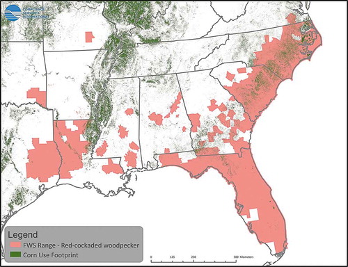
Data are needed to characterize location, and time/date, activity classifications (foraging, flying, resting, etc.), and environmental conditions to refine understanding of where, when, how often, and how listed species interact with agricultural areas. Refined spatial analysis combining listed species radiotracking data and crop-specific use data can and should be incorporated at early stages of tiered approaches designed to assess risks associated with listed species utilization of agricultural settings at specific times and locations to avoid unnecessary investments of time and effort.

7.2 Other lines of evidence

There are several lines of evidence that can be used to verify conclusions from screening for direct effects of atrazine among non-target terrestrial animals. These are rarely associated with listed species but lack of effects in animals in the same taxon can provide confirmation of lower-tier decisions to exclude or include listed species from further assessment.

Conservative evaluations of specific pesticide risk may appropriately contain thorough consideration of incident data with special attention given to MA species and their taxa as identified in Step 1 of the ESA ERA process. Incident reports linking adverse effects among birds, mammals, invertebrates, and other taxa to pesticide usage are compiled in several databases including the Ecological Incident Information System (EIIS), Incident Data System (IDS), and the Avian Incident Monitoring System (AIMS). Searches of available data reveal no substantiated incident reports linking atrazine alone to adverse incidents involving any avian species.

In response to the USEPA’s 2016 assessment (USEPA 2016), the registrant obtained incident data for atrazine from the Ecological Incident Information System (EIIS) and Incident Data System (IDS) in August 2016 via FOIA request (Syngenta 2016c). Incident data reach back as far as the early 1970s identified one probable incident with a wild bird species (Canada goose), two incidents with an unknown bird species and two involving chickens. Those incidents were not definitively attributed to atrazine, as other, more toxic agents were used concurrently. Two of the incidents involved misuse of atrazine. In addition, another database (the ProPharma database, see SI Section 5) was queried. There, two possible incidents involving birds and atrazine were listed; a rooster and a hen were found dead following application of a formulated herbicide containing atrazine to a field, and three birds were found dead 300 yards from a field wherein multiple herbicides had been sprayed (one containing atrazine). Neither of these incidents included confirmation of exposure to atrazine or intoxication as the cause of mortality. Incident reports from the AIMS are no longer accessible, and multiple requests to the sponsoring nongovernmental organization (American Bird Conservancy) have yielded no data.

As is the case for birds, there are no adverse incidents reported in the EIIS database for any wild mammals, listed or not. Adverse incidents involving atrazine and domesticated mammals have been reported wherein cattle, horses, and/or dogs were exposed via ingestion of undiluted formulated product (SI Section 5). Likewise, there are no incident reports describing serious adverse effects on terrestrial invertebrates. However, one incident report suggests that bees within an application area were knocked out of the air following aerial application of atrazine and a liquid form of nitrogenous fertilizer (see SI Section 5), but it is unclear whether the bees experienced toxicity or were simply wetted to the point they were unable to fly. There was no other incident reported for terrestrial invertebrates.

When considered in total, incident reports for atrazine indicate no adverse effects of atrazine on wild or listed terrestrial mammals, birds, or invertebrate species when stored or applied using good agricultural practice.

7.3 Direct effects of atrazine on terrestrial animals

EPA’s refined atrazine risk assessment relied on acute and chronic toxicity data generated from surrogate species from broad taxonomic groups to extrapolate potential direct and indirect effects related to survival, growth, or reproduction among species within the same taxon (USEPA 2020e). The following is a brief discussion of toxicity data identified by EPA as acceptable and relevant to qualitative and quantitative assessment of risks to terrestrial invertebrates, birds, and mammals since these data form the basis for evaluation of risk to listed species.

7.3.1 Direct effects of atrazine on terrestrial invertebrates

In its draft Biological Evaluation, USEPA (2020b) concluded that, in all but one case, direct effects from atrazine would not be expected in terrestrial invertebrates and animals in soil such as earthworms. The LD50 for honeybees (Apis melifera) is >97 µg/bee (Table 1–2 in USEPA 2020b). Direct exposure of honeybees to atrazine is unlikely because of the preplant or early postplant application but flowering weeds might be present in no-till fields. Non-Apis bees have not been tested for sensitivity to atrazine; however, a new study has indicated that honeybees are good surrogates for adverse effects in wild bees, so they are also unlikely to be affected (Thompson and Pamminger 2019). Although residues of atrazine have been detected in pollen and wax from honeybee colonies (Mullin et al. 2010), (95th centiles in wax and pollen were <20 µg/kg) responses to exposures in brood have not been reported.

7.3.2 Direct effects of atrazine on mammals

The most sensitive endpoints for mammalian acute exposure identified and selected for use in the draft Biological Evaluation of atrazine (Table 1–2 and 2–2 in USEPA 2020b) indicate low risk of lethality. The registrant’s comments on USEPA’s 2016 ERA (Olson et al. 2016) point out several issues. These include the preferred use of chronic toxicity based on the dietary route of exposure, the problem with conditioned taste avoidance (CTA) of food intake by atrazine and its metabolite DACT (Figure 3), which, as discussed below, is relevant to the use of weight loss as an endpoint for risk assessment and the choice of an appropriate NOAEL as a point of departure for assessing risks.

The most sensitive endpoints for mammals identified and selected for use in the 2016 USEPA ERA for Atrazine were 1,869 mg/kg-bw (acute mortality) and 50 mg/kg-diet (chronic sublethal) based on alterations in body mass and food consumption (Mainiero et al. 1987; Sachsse and Bathe 1975). Appropriately, the USEPA (USEPA 2015a) has stipulated that, for critical endpoints based on direct effects derived from sublethal endpoints, only those that can be linked to environmental (e.g., dietary) exposures are to be considered. The direct effect, sublethal NOEL endpoint (50 mg a.i./kg diet; weight) selected for atrazine by EPA (USEPA 2016) was derived from a study in which Norway rats (Rattus norvegicus) were administered atrazine via diet at concentrations of 0, 10, 50, or 500 mg a.i./kg diet. The author of that study (Mainiero et al. 1987) reported reduced food consumption in F₀ and F₁ males and females fed 500 mg a.i./kg atrazine, which was accompanied by reduced body weight and body weight gains. The 50 mg a.i./kg NOEL treatment was an order of magnitude lower than the highest dose, which may have resulted in an overly conservative NOEL value.

Exposure of laboratory rodents to atrazine via the diet better approximates potential exposure among wild mammalian listed species. Dietary exposure in laboratory settings, though it encourages gradual and continuous exposure and accounts for the food matrix effects on toxicokinetics of the test chemical, does not adequately allow for dietary selection/discrimination among experimental animals. It is interesting to note that CTA has been documented in 60-day-old male Wistar rats orally gavaged with atrazine (single dose) as low as 25 mg/kg (Hotchkiss et al. 2012). A single 50 mg/kg dose significantly decreased food intake in as little as 6 h in the same study. Similarly, administration of DACT, a metabolite of atrazine, resulted in CTA in rats at a concentration equimolar to an atrazine dose of 200 mg/kg. Should the mechanism or mechanisms producing CTA responses to atrazine and its metabolites be additive or synergistic, it is possible that exposure to atrazine and/or DACT in wild mammals is self-limiting.

The Hotchkiss et al. (2012) study provides important perspective on the chronic sublethal mammalian critical endpoint selected by EPA for use in its refined risk assessment (USEPA 2016). First, given evidence for development of CTA at half the selected critical endpoint dose, chronic exposure to doses of 50 mg/kg/day among mammals in the environment is unlikely. Secondly, if CTA occurs in laboratory studies wherein rodents are exposed to atrazine via food, then weight gain and food intake may not be suitable endpoints for assessing risk posed by atrazine or they may yield confounded data. Thus, selection of weight-related measures as critical chronic, sublethal endpoints for mammals exposed to atrazine is questionable based on their transient nature and evidence of CTA.

Another chronic NOEL value for weight or weight gain in mammals exposed to atrazine via diet contained within the EPA ECOTOX database is 70 mg/kg diet in Sprague-Dawley male and female rats exposed for 104 weeks (Stevens 1999), 40% higher than that identified in EPA (2016). Like the Maniero et al. (1987) study, the next highest dose (LOEL) for changes in weight or weight gain identified by Stevens et al. (1999), was 500 mg/kg diet. Stevens et al (1999) also reviewed several studies in which rats and mice were exposed to atrazine via diet, and reported that significant reductions in weight, weight gain, and food consumption were evident, but only in concentrations exceeding 300 mg/kg diet. Thus, it is likely that the actual NOEL for weight/weight gain in mammals exposed to atrazine via diet is ≥70 mg a.i./kg.

7.3.3 Direct effects of atrazine on birds

The USEPA’s 2016 assessment listed the most sensitive endpoints for acute and chronic toxicity tests on birds (Table 53 in USEPA 2016) and concluded that atrazine is only slightly acutely toxic. USEPA used several models of different complexity to assess possible risks to birds from chronic exposures. The Terrestrial Residue EXposure Model (T-REX)³ is a screening-level model which estimates dietary exposure of birds assumed to feed on one dietary item, 100% of the time (USEPA 2012f). This Tier I model uses the estimated exposure values and applies them with threshold toxicity values to calculate risk quotients (RQs).

The Terrestrial Investigation Model (TIM) includes dietary, inhalation, water, and dermal routes of exposure to calculate impacts on survival of birds (USEPA 2015b). This probabilistic modeling approach allows for estimating exposure from multiple dietary items and can include relevant half-lives for different food items. Outputs of this model include probability of survival as well as estimated daily doses (EDD). For chronic effects, TIM is integrated with the Markov Chain Nest productivity model (MCnest), a mechanistic model of avian breeding phases to assess impacts of exposure on annual reproductive success of exposed birds (Bennett and Etterson 2007). MCnest is parameterized for more than 50 species, mostly focusing on farmland, rather than listed, species, though some recent applications of the model were for assessments of listed species. The MCnest model explicitly simulates breeding activities of a population of females each day through the breeding season. Breeding activity is described by a series of phases, including pairing and selection of breeding site, production of eggs, incubation to hatching, rearing of nestlings, and fledgling.

Impacts of exposure to a pesticide on the breeding activities are modeled via either T-REX or TIM, though the integration with the latter model is more commonly used. TIM calculates EDDs which are then used to establish risk quotients for each of the breeding phases. The toxicity endpoints are based exclusively on data from Northern bobwhite and mallard. If any of the calculated risk quotients are >1, then that specific phase fails, and that specific bird experiences a failed breeding attempt that season. However, if time permits, birds can restart the breeding cycle and re-attempt to complete all reproductive phases.

As an example, the integrated TIM-MCnest model was applied to assess risks from 12 insecticides to 31 farmland species of birds and showed differing predictions on reductions in fecundity and survival depending on the date of the first application of the insecticide (Etterson, Garber, and Odenkirchen 2017). The model was also applied for atrazine risk assessment. However, many of the input values that USEPA (2016) chose for their models in the 2016 ERA either did not follow their own guidance or were not appropriately determined from studies submitted by the registrant and/or the scientific literature (Olson et al. 2016). Furthermore, the models used by EPA incorporated several overly conservative assumptions that should not have been used in a refined risk assessment. These errors were communicated to USEPA in detail by the registrant (Olson et al. 2016).

7.3.4 Field observations of effects of atrazine on birds

While understanding that the modeling is designed to estimate risk for individual birds, USEPA should also consider the population data available from the USGS Breeding Bird Survey (BBS) in areas of high use of atrazine. With the input parameters for exposure and life history from the preliminary atrazine risk assessment (USEPA 2016), the TIM-MCnest model estimated 22.2% mortality within a vesper sparrow population and complete reproductive failure for scenarios in which high use of atrazine occurred. The lack of incident data (see Section 7.2 above) indicates that the TIM-MCnest modeling over-estimated exposure to and effects of atrazine in birds. In addition, abundance of vesper sparrows reported in the BBS for Illinois indicate a steady population trend over the period of 1966 to 2013. Annual indexes are estimated as yearly predicted abundances (Sauer et al. 2014). Although direct linkage between survey data and precise locations of atrazine use cannot be made, the extent of the spatial (State of Illinois) and temporal (47 years) overlap between high use of atrazine and monitoring of populations provides context to indicate that the modeling output predicted for each use event is not reflective of long-term broader population trends. The BBS also quantifies use of land within 0.4 km (0.25 mile) on each side of a survey route. Thus, data for land cover were explored for the 103 BBS survey routes in Illinois (data for land cover were available for 102 of 103 IL routes). These data indicate that, of the land-use within the survey routes, row crops comprised an average of 56.9% of habitat area surveyed. This further strengthens the linkage between BBS survey data and areas of high use of atrazine and indicates that TIM-MCnest modeling predictions are inconsistent with long-term population trends.

In two other examples (as highlighted in Olson et al. 2016), trend maps from the BBS data for Killdeer (Charadrius vociferous) and chipping sparrow (Spizella passerina) in the USA from 1966–2013 were compared to the results of modeling used by the USEPA. The TIM-MCnest model indicated significant mortality and no reproduction in atrazine use areas, yet the BBS trends indicate long-term population increases in these species in regions of high use of atrazine. Thus, when considering the spatial and temporal extent of population monitoring in the BBS, TIM-MCnest modeling output is not reflective of long-term avian population trends in regions in which the use of atrazine is high.

Following this line of evidence, more in-depth analysis was conducted on population trends of birds commonly found in mid-west US agroecosystems (Belden et al. 2018). The goal was to test the hypothesis that agricultural intensification and associated factors such as use of herbicides correlated with declining bird populations across the United States. The study used spatially explicit USDA National Agricultural Statistics Service’s CDLs and data on abundance of birds from the BBS from 1995 to 2016 (i.e., during periods of intensive use of atrazine). Temporal trends (i.e., slopes) of population count data for 31 avian species were compared between grassland- and cropland-dominated landscapes and across varying intensity of mixed corn and soybean land-cover. Almost all species showed significant population-level responses to changes in land-cover. However, foraging guild or taxonomic relationships did not explain whether species responded either positively or negatively and negative trends were not observed across a broad spatial scale nor across most species. If the widespread use of atrazine within the spatial scale of this study was impacting avian populations to the degree predicted by the TIM-MCnest mechanistic model, the results would have indicated across-species and/or within guild patterns. These patterns were not observed; there was no broad general trend of greater avian population declines in crop-intensive areas suggesting that processes other than use of pesticides were responsible.

7.3.5 Refinements to the TIM model

An additional refinement of past higher tiered avian assessments for atrazine involved modeled avian dermal exposure estimates (Maul, Blackstock, and Brain 2018). Specifically, within USEPA’s 2016 ERA (USEPA 2016), the TIM model was used to estimate avian dermal LD50 values and dermal exposure. For atrazine, the output resulted in extremely high dermal exposure and low dermal LD50 estimates. It was determined that the TIM model used data on toxicity of organophosphorus and carbamate insecticides, which have very different toxicokinetic and toxicodynamic properties from atrazine, to estimate the relationship between oral and dermal toxicity. Furthermore, this component of the model was determined to be inappropriate by a 2004 EPA SAP. Maul, Blackstock, and Brain (2018) have demonstrated a new approach for estimating avian dermal LD50 values and refining predicted dermal exposure within the TIM model using empirical data generated from experiments on dermal absorption of atrazine conducted with skin of mallard duck, northern bobwhite quail, and rats. This approach of using refined model input parameters resulted in a smaller total body-dose of atrazine, a smaller dermal fraction of the total atrazine dose, and reduced predicted mortality from dermal exposure to atrazine. Furthermore, previously proposed methods to solve this problem (i.e., use of mammalian data and physico-chemical properties) were confirmed. That is, the three alternative approaches for estimating dermal exposure to atrazine in birds that were described in Maul, Blackstock, and Brain (2018) resulted in consistent predictions that were all different from the output of the current TIM model.

In addition to the dermal LD50 estimate and dermal exposure refinement described above, several simple inputs into the TIM model were incorrect. These included an inappropriate estimate of the hourly fraction retained by birds (i.e., the mammalian elimination kinetics for fraction of DAC retained was not used) and the incorrect probit slope for the dose–response data was used as input. Here, the recalculated LD50 from the USEPA’s data evaluation record (DER) analysis was used but this was combined with the slope from the original analysis and used as inputs into TIM. Considering these three refinements, the predicted mortality from TIM for a model passerine species for corn/soybean agroecosystems (i.e., vesper sparrow [Pooecetes gramineus]) changed from the original EPA ERA conclusion of 22.2% mortality to <0.00001% mortality with only the three refinements described above.

7.4 Indirect effects of atrazine on birds, terrestrial invertebrates, and mammals

7.4.1 Field studies on indirect effects of atrazine on terrestrial animals

Indirect effects of herbicides on non-plant organisms in edge-of-field habitats may manifest as loss or reduction in abundance or fitness due to loss of habitat and food resources when plant habitat is degraded or lost (Prosser et al. 2016). With reference to herbicides, indirect effects from off-field habitat and alterations in food resources represent greater risk to terrestrial invertebrates, birds, and mammals than do direct effects (Prosser et al. 2016) but are more difficult to quantify. Nonetheless, indirect effects on edge-of-field habitats should be considered when assessing risks posed by herbicides to critical habitats of listed species. Almost all attempts to characterize indirect effects of herbicides extrapolate from direct overhead spray studies to off-field, or edge-of-field plant communities thereby misrepresenting the way off-field exposures occur, and subsequently overestimate risk of exposure. This issue is discussed further in Section 3.3.2. Another complication is that herbicidal effects in the margins of the field may be conflated with other agricultural activities, such as mowing, disking, irrigation, roads, etc. In addition, contemporaneous use of fertilizers, fungicides, defoliants, and insecticides present a significant challenge; singular use of herbicides without other mechanical or agrichemical landscape manipulations is rare.

Definitive assessments of indirect herbicide effects on animals inhabiting or using field margins are scarce (Prosser et al. 2016). Thus, qualitative assessments are often necessary. Prosser et al. (2016) conducted an in-depth review of published literature that addressed indirect effects of herbicides on terrestrial invertebrates, birds, and mammals in agricultural edge-of-field habitats. As testament to the complexity of and (to date) limited understanding of this issue, only 29 peer-reviewed papers were identified and selected for review. None of these addressed effects of atrazine on listed species.

Only one field study was identified by Prosser et al. (2016) that specifically examined indirect effects of application of herbicide on abundance and diversity of plants and butterflies. Following direct application of glyphosate to field margins, Feber, Smith, and Macdonald (1996) documented reduced abundance and species richness of butterflies, presumably related to reduced abundance of flowers and sources of nectar. Clearly, direct application of broad-spectrum herbicides (e.g., glyphosate) and broadleaf-selective herbicides to field margins has potential to cause indirect effects in butterflies foraging in field-margins by reducing nectar-producing plant species and reducing availability of plant species that serve as obligate hosts for butterfly larvae (e.g., Monarch butterflies and milkweeds). An important distinction is that indirect effects resulting from normal, in-field agricultural use of herbicides such as atrazine at field application rates should not be equated with or extrapolated from intentional applications of herbicides to field margins.

Herbicides in general may also indirectly affect listed coleopterids, or coleopterid species that serve as important prey items for listed birds occurring in edge-of-field habitats. Herbicide-induced reduction in habitat canopy structure with concomitant changes in microhabitat conditions (e.g., temperature, humidity, etc.) can reduce abundance of carabid beetles or their prey. Delayed (21-day post-application) reductions in abundance of carabid beetles relative to controls were noted in plots treated with atrazine at the recommended field rate of 2.24 kg a.i./ha but were not statistically significant (Brust 1990). The review by Prosser et al. (2016) included several studies with larvae of beetles feeding on non-target plants exposed to herbicides at field application rates that could result in adverse indirect effects but noted that these were unlikely when edge-of-field plants were exposed to herbicides below field application rates as would occur from spray drift. The lack of biologically relevant exposures of plants in field margins with appropriate buffers (see Section 3.3.2) indicates that this is not a significant concern regarding effects of atrazine and any plants in field margins, obligate food sources, or not.

An extension of the Brain et al. (2019) herbicide drift study that included measurements of altered dynamics in the plant community in conjunction with abundances of invertebrates and seeds, and that monitored avian and mammalian use in reference to unsprayed reference habitats would greatly enhance our understanding of potential indirect effects on listed terrestrial species.

7.4.2 Use of population models to characterize potential indirect effects of atrazine on listed mammals

Population models of listed mammals have not yet been applied to assess risks from exposure to atrazine or any other crop protection product. Existing models have mainly been used to investigate and quantify impacts of physical habitat alterations, i.e., habitat loss and fragmentation, harvesting/hunting, and biological stressors, including predation, competition, or disease, on the persistence of listed mammal populations such as, gray wolves (Canis lupus) (Carroll et al. 2006), ocelot (Leopardus pardalis) (Haines et al. 2006), black-footed ferret (Mustela nigripes) (Shoemaker et al. 2014), and the Indiana bat (Myotis sodalis) (Thogmartin et al. 2013). All these models could potentially be applied to assess direct or indirect effects of atrazine on population persistence, but modifications and additional data are needed. For instance, the indirect effect assessment would require additional information about the impacts of atrazine on dynamics of prey items. Nevertheless, these tools are available for a subset of species and could be further developed and applied to assess risks from exposure to atrazine and to other stressors, including loss of habitat and disease. Given the lack of exposure of carnivores either directly or via the food chain (Table 9), direct and indirect effects are unlikely in this group of mammals.

7.5 Strengths and uncertainties

It is well established that atrazine is among the most intensively studied agrochemicals ever produced such that its physicochemical properties, fate and transport, mechanism of action, use patterns, environmental occurrence, and toxicity profile are readily available to inform risk determinations associated with conservation of listed species. Appropriately, federal agencies are mandated to evaluate actions they authorize including Section 7(a)(2) of the Endangered Species Act. With specific regard to pesticide registrations, the USEPA, in consultation with USFWS and NMFS, must evaluate potential impacts to federally listed threatened or endangered species and their designated critical habitats. However, guidance for implementation of listed species/pesticide-related risk assessments would benefit from continued refinement, especially Step 1, which in effect, serves as a screening-level assessment. Current procedures for Step 1 are so conservative that, few, if any listed species can be designated as NE species for widely used pesticides due to limitations associated with listed species-range and habitat selection data. Recent acknowledgment that factors such as dormancy periods, migration patterns, precision of species-ranges, and seasonal dietary considerations can be considered when distinguishing between NLAA and LAA in Step 2 indicate progress, but more are needed. More emphasis and refinement relative to habitat selection/affinity among listed species are important considerations that should be integrated early in the listed species risk assessment process. Incorporation of available georeferenced habitat selection data with crop-layer data and geospatial data for product use would significantly improve the initial screening process.

Conservative approaches are justifiable when implementing strategies to protect threatened and endangered species, but conservatism should be tempered by best available science and robust data where it exists. As an example, uncertainty and overly conservative parameterization of the AGDRIFT model results in extreme overestimates of pesticide drift when compared to empirical drift values derived by Brain et al. (2019) that significantly clarifies deposition in the field border areas of concern. Similarly, critical endpoint selection should be protective of listed species taxa, but not simply based on lowest available values. NOEL and LOEL values are artifacts of study design, and not true representations of toxicity thresholds. In addition to study design, exposure medium and avoidance/aversion of the test agent should be considered, especially when growth-related endpoints are selected. Further, selection of rodent toxicity values as critical endpoints may not adequately reflect sensitivity of the listed mammal species.

In terms of available exposure and effect models for birds, there are several uncertainties within screening and higher-tiered models that have led to unrealistic conclusions related to risk of atrazine. These have ranged from simple incorrect inputs (e.g., inappropriate estimate of the hourly fraction retained by birds and an incorrect probit slope used in TIM-MCnest) to mechanistically incorrect exposure calculations (e.g., how the dermal to oral toxicity ratio is calculated in TIM). In addition, these models include many inputs, each with overly conservative assumptions leading to a significant compounding of conservatism. Examples of conservative assumptions include: the amount of diet obtained from a treated field is 100%, residues on all feed items are from direct spray, all foliar dissipation half-lives are 35 d, chronic endpoints are compared to peak acute exposure estimates, organisms consume 100% of one of a variety of dietary items (short grass, tall grass, broadleaf plants, arthropods, seeds/grains or fruits, pods, or seeds) as opposed to a mixed item diet, etc. The combination of input errors, incorrect model mechanisms, and compounding of highly conservative assumptions have led to unrealistic model output that is used to inform regulatory decisions. Furthermore, output from the higher-tiered model TIM-MCnest suggests significant impacts of atrazine to reproductive endpoints that would theoretically lead to significant population declines. However, as discussed above (Section 7.3.4) these predictions are inconsistent with avian census data over a time frame of extended use of atrazine use.

Despite the robustness of the atrazine ecotoxicological data repository, data gaps exist which limit thorough evaluation of risk among listed species. Limited data (relative to other taxa) exist for toxicity of atrazine to terrestrial invertebrates, such as butterflies. Likewise, there are very few field studies available in the literature wherein the effects of atrazine are directly attributable to atrazine and not to other co-applied pesticides (see SI Section 5 and (Prosser et al. 2016) and/or mechanical manipulations of the field and field-border.

8 Stewardship and mitigation of potential effects of atrazine on listed species

Although this perspective did not identify any unacceptable risks from the use of atrazine to listed or non-listed species in the conterminous United States, it is prudent to ensure that mitigation measures are available and followed by users. Mitigation can be achieved by several means, namely regulatory, technological, and stewardship, all of which are focused on reduction of exposure of non-target organisms.

Regulatory mitigation can be achieved by government regulators i.e., removing or restricting the registered uses of a product where necessary and/or appropriate, but can also be invoked by the registrant via proactive voluntary restrictions and requirements on the product label that have been accepted by USEPA¹³ (Syngenta 2020). The label is essentially a legal document and, under rules of good agricultural practice, must be followed. Syngenta Crop Protection LLC had proposed several regulatory changes (off-labeling) that, now they are accepted, have mitigated exposure of non-target organisms in certain regions. These regions are:

• Hawaii

• U.S. territories (Puerto Rico, Guam, American Samoa, the U.S. Virgin Islands, and the North Mariana Islands).

Atrazine had few uses in these regions and these uses were either declining due to shifting agronomic factors or covered a very limited geography. For example, sugarcane production had essentially ceased in Hawaii and the territories (i.e., Puerto Rico); 435 tons of sugarcane was harvested in Hawaii in 2017 compared to 7,934,181 tons in 1987 (USDA 2019). Moreover, Hawaii, has 437 listed species of plants and animals¹⁴ and this action has essentially reduced potential exposures and potential risks from atrazine to all these species to zero. Atrazine was not registered for use in Alaska so these changes in labels have restricted the use of atrazine to the conterminous United States. Further, within the conterminous U.S., Syngenta has no active registrations in California which contains 283 threatened and endangered species.¹⁵

Uses on fallow lands have been restricted to the following scenarios and geographies only:

Wheat-Corn-Fallow in CO, KS, ND, NE, SD & WY

Wheat-Fallow-Wheat in CO, KS, ND, NE, SD & WY

Wheat-Sorghum-Fallow in AR, CO, GA, IL, KS, LA, MS, MO, NE, NM, NC, OK, SD & TX

Other uses that have been off-labeled include weed management on roadsides and rights of way, use on Conservation Reserve Program lands, and uses in forestry. All these uses had either ceased or were declining and represented a small fraction of atrazine applied. These changes in labels will reduce potential exposures and risks for listed species in action-areas for these uses to zero.

Technological mitigation is already required on the label for atrazine and will be retained. These mitigation measures are aimed at protecting surface-waters from possible contamination and are:

• “This product must not be mixed or loaded within 50 feet (15.5 m) of intermittent streams and rivers, natural or impounded lakes and reservoirs.”

• “This product may not be applied aerially or by ground within 66 feet (20 m) of the points where field surface water runoff enters perennial or intermittent streams and rivers or within 200 feet around natural or impounded lakes and reservoirs.”

• “If this product is applied to highly erodible land, the 66-foot (20 m) buffer or setback from runoff entry points must be planted to crop, seeded with grass, or another suitable crop.”

The last point is discussed in Section 6.2.2 of this perspective and several published studies have shown that is effective in reducing runoff.

Beyond these existing measures, additional spray drift mitigation measures have been incorporated in the atrazine label. These are based on a recent field-based spray drift bioassay (Brain et al. 2019), which measured exposure and effects under worst-case conditions discussed in Section 3.3.2. They will provide the following mandatory directions to reduce spray drift:

• Use nozzles intended to deliver a coarse to ultra-coarse droplet size distribution.

• Do not apply if average windspeeds exceed 10 mph (16 km/h) for ground or 15 mph (24 km/h) for aerial applications.

• Use a maximum release height of 4 feet (1.2 m) for ground applications and 10 feet (3 m) for aerial applications.

• Maintain a 15-foot (4.6-m) in-field downwind buffer from critical habitat for threatened and endangered species and/or species locations for ground applications and a 150-foot (46-m) buffer for aerial applications. These buffers would also apply generically to the edge of streams and rivers as well as the high-tide line for estuarine/marine environments. Bulletins Live¹⁶ can be utilized to identify counties with potential co-occurrence of listed species and registered uses.

Product stewardship should continue with the added commitment to explore net conservation offset approaches in order to translate potential ecological risks to listed species into monetary investments for habitat improvement where feasible and appropriate. Such methodologies could potentially include some form of mitigation bank credits, permittee responsible credits, and in-lieu fees.

9 Conclusions

Atrazine is a widely used herbicide that has been on the market since initial registration in the late 1950s. During this time, under FIFRA as administered by the USEPA, it has been subjected to multiple data call-ins, a Registration Standard (1983), a Special Review (1994), Re-Registration Reviews (2003 and 2020/currently) and 13 Scientific Advisory Panels (five directly focused on ecological issues). Many studies related to the environmental fate and effects of atrazine have been conducted by the registrant and independent entities prior to publication in the open scientific literature. It is arguably the most studied pesticide and correspondingly there is a wealth of data available, much of which can be applied to assessment of potential effects in, and risks to, endangered and threatened (listed) species. This perspective was focused on key issues that should be considered in risk assessments of atrazine under the purview of the current US Endangered Species Act (ESA). Several key conclusions that are relevant to this ESA assessment are highlighted here.

Atrazine is a nonselective inhibitor of photosynthesis, a biochemical process unique to plants and some photosynthetic bacteria and is not expressed in animals. Thus, the likelihood of direct effects in exposed plants should be the primary concern in any assessment of listed or non-listed species. Photosynthesis is a highly conserved process in plants and there is no evidence to suggest that listed plant species are inherently more sensitive to herbicides than non-listed plants. Therefore, it allows for the extrapolation of responses from the many studies on non-listed plants to listed species, few of which have ever been tested.

Likewise, it is important to understand that atrazine does not bind covalently at the target site in plants, thus its mechanism of action is reversible. When exposure concentrations decrease, plants recover as photosynthesis resumes unless energy reserves are overly depleted. Concentrations of atrazine at target sites in the plant can decrease either via metabolic breakdown or, for aquatic plants, if the concentration in surrounding water decreases such that atrazine partitions from the plant into the water thereby initiating recovery. This has been demonstrated in numerous laboratory and semi-field studies.

In terms of direct effects in animals, these will likely only be observed at doses or concentrations much greater than those that affect plants. Because atrazine has low affinity for lipids, it will not accumulate in tissues of herbivores that consume treated plants, and it does not biomagnify in food chains. This simplifies characterization of exposure pathways for listed and non-listed species: for carnivores, invertivores, and fungivores, atrazine exposure pathways are essentially incomplete or so small as to be toxicologically insignificant.

Regardless of whether any plant or animal is sensitive to atrazine or not, exposure must occur before there is potential for any type of response. For example, based on atrazine use patterns in the US, the seven listed species of aquatic plants would not be exposed to atrazine at concentrations sufficient to cause direct adverse effects. As well, since the 1980s, numerous monitoring programs have characterized atrazine residues in surface waters. As part of the 2003 reevaluation, the Atrazine Ecological Monitoring Program was mandated for selected watersheds representing worst-case runoff scenarios for atrazine in the US. These data reflect daily or near-daily monitoring of surface water from locations that represent the upper 80th centile of vulnerability to storm-induced runoff. Analysis of these data from 2004 to 2018, the most representative period for current atrazine use-patterns, revealed that the 99th centile rolling average daily, 4-d, 21-d, and 60-d concentrations were 53, 24, 20, and 18 µg/L, respectively. Comparing these concentrations to the thresholds for effects measured in numerous laboratory and semi-field studies on plants and animals provides a useful context for assessing worst-case risks that are protective of listed species.

The accuracy of geospatial information regarding locations and ranges of listed species and their critical habitat is limited compared to the spatial and temporal use of atrazine, increasing uncertainty and complicating assessments. Consequently, there is a compelling need for more precise and accurate geospatial data to resolve this issue. Moreover, listed species proximity evaluations should be informed by, and refined from, relevant experimental data for both potential direct, and indirect, effects. New field-scale studies on spray drift provide evidence of lack of biologically significant off-target movement of atrazine beyond 4.6 m (15 ft) from the edge of the spray-swath. These data provide useful information for establishing downwind buffers/setbacks derived under worst-case conditions (e.g., windspeeds >16 km/h (10 mph), bare ground, highly sensitive test species) that are protective of potential direct effects on sensitive plants, as well as indirect effects to listed animals relying on plants for food, shelter, and refugia. These experimentally-derived buffers offer protection from direct and indirect effects in listed and non-listed plants and other non-target organisms in margins of fields.

Potential direct and indirect effects of atrazine on plants and/or animals have been studied at the community level in aquatic systems and would only be expected to occur at unrealistic exposure concentrations and durations that are unlikely to occur in the field, even in worst-case scenarios of use. There is less experimental evidence and therefore more uncertainty for indirect effects in terrestrial systems. However, the few studies that have been reported do not suggest adverse effects on beneficial invertebrates and other organisms that inhabit off-field areas. In addition to the evidence-based downwind buffers, other techniques to mitigate off-field movement, such as vegetative buffer strips, can provide viable mechanisms to reduce exposures of listed and non-listed species.

We find that incident reports are among several lines of evidence that add confidence to conclusions drawn from screening for direct effects of atrazine on non-target organisms. Despite limitations, and although incident reports only exist for non-listed species, those pertaining to organisms in the same taxon could serve to confirm conclusions of MA and NE. In our assessment of available incident data, none of the corroborated incidents were associated with diluted spray solution and were most often caused by misuse of concentrated material. We acknowledge the inherent challenges associated with voluntary incident reporting databases, which include reporting bias (both conscious and unconscious), carcass visibility, temporality, and potentially related causal observations. Such data sources could provide a useful basis for relative comparison. However, it is important to use these data within context and consider factors that drive the quality of incident data such as probabilities of detection.

We note that there have been major advances in modeling effects of pesticides at the population and community level, but some knowledge gaps still exist. For atrazine, like other pesticides, these gaps include the distribution of listed species and locations where the product is used. For listed and non-listed species, there is also a need to ensure that exposure and effects models used for regulatory assessment are parameterized appropriately before they are used a basis for decision making. There is also a compelling need to improve the accuracy of geospatial information on the locations and ranges of listed species in relation to the spatial and temporal use of atrazine for management of weeds.

Lastly, several technical measures for mitigation of potential risks of atrazine to listed and non-listed species have been proposed by the primary registrant (Syngenta). In addition to current guidance for use on the product label, additional mitigation measures, including new directions on spraying have been proposed to the USEPA. These include the use of nozzles that deliver a coarse to ultra-coarse droplet size distribution and revised downwind buffers. Moreover, Syngenta has off-labeled the use of atrazine for certain geographies including Hawaii, Puerto Rico, Guam, American Samoa, the US Virgin Islands, and the North Mariana Islands due to declining use and significant numbers of endemic listed species. In addition, several uses, such as forestry, roadsides and rights of way, and Conservation Reserve Program lands have been off-labeled in the USA. These actions will significantly reduce the number of listed species (by about 500) potentially exposed to atrazine and will simplify the assessment of potential effects on other listed species.

Based on the totality of scientific evidence evaluated herein, coupled with the proposed mitigation measures regarding use patterns, geographies, and application specifications, the available data indicate that atrazine is not likely to cause adverse effects in listed species at environmentally relevant exposures. This conclusion is based on a wealth of data on atrazine collected over 60 years and represents the most comprehensive data sets for both exposure and effects of current-use herbicides.

Declaration of interest

All authors contributed equally to writing of the paper and the SI. RAB, WC, NG, LG, and JM are employees of Syngenta Crop Protection, LLC, Greensboro, NC, USA. PNS, KLA, JMG, MLH, GVDK, and KRS were contracted as consultants to Syngenta Crop Protection to provide an independent perspective of the material considered. The opinions expressed in this paper are those of the author(s). Any mention of trade names or commercial products should not be interpreted as a recommendation for use.

Acknowledgments

The authors thank Syngenta Crop Protection Inc. for providing access to reports and raw data. We also thank Farah Abi-Akar of Waterborne Environmental for conducting the AgDrift modeling discussed in Section 3 above and, in more detail, in SI Section 4 ([email protected]) and Compliance Services International (CSI) for geospatial analyses and mapping support.

Supplementary material

Supplemental data for this article can be accessed on the publisher’s website.

Additional information

Funding

This work was supported by the Syngenta Crop Protection LLC.

Notes

1. Intensive properties are physical and chemical properties of a substance that are independent of concentration, such as density, partitioning, solubility, and reactivity with other substances. Extensive properties are those that are dependent on concentration such as mass and toxicity.

2. FIFRA defines the term ‘‘unreasonable adverse effects on the environment’’ to mean: ‘‘(1) any unreasonable risk to man or the environment, taking into account the economic, social, and environmental costs and benefits of the use of any pesticide, … ” https://www.epa.gov/laws-regulations/summary-federal-insecticide-fungicide-and-rodenticide-act

3. https://www.epa.gov/pesticide-science-and-assessing-pesticide-risks/models-pesticide-risk-assessment

4. https://www.epa.gov/pesticide-science-and-assessing-pesticide-risks/terrplant-version-122-users-guide-pesticide-exposure

5. https://www.regulations.gov/document?D=EPA-HQ-OPPT-2009-0154-0024

6. https://www.regulations.gov/document?D=EPA-HQ-OPPT-2009-0154-0023

7. (https://www.youtube.com/watch?v=Uxw5WBl0stM&t=39s)

8. Depending on the HUC and bin (aquatic scenario; bin 1 is a seasonal wetland, flowing aquatic bins include bin 2 [low flow], bin 3 [moderate flow], and bin 4 [high flow] and static aquatic bins include bin 5 [low volume], bin 6 [moderate volume], and bin 7 [high volume] etc.).

9. https://plants.usda.gov/core/profile?symbol=AMPU7

10. https://www.epa.gov/caddis-vol4/caddis-volume-4-data-analysis-download-software

11. The no-observed adverse effect rate of deposition (NOAERD) in mass per unit area would be a more appropriate measure of exposure of the plants. Similarly, the rate of deposition causing a specified percentage reduction in relative growth rate would be better than the effective concentration.

12. https://www.fws.gov/rcwrecovery/rcw.html

13. https://www.regulations.gov/docket?D=EPA-HQ-OPP-2013-0266

14. https://www.fws.gov/pacificislands/species.html

15. https://ecos.fws.gov/ecp0/reports/species-listed-by-state-totals-report

16. https://www.epa.gov/endangered-species/bulletins-live-two-view-bulletins

References

- Albright, V. C., III, I. J. Murphy, J. A. Anderson, and J. R. Coats. 2013. Fate of atrazine in switchgrass–soil column system. Chemosphere 90 (6):1847–53. doi:10.1016/j.chemosphere.2012.09.097.
- Aldenberg, T., J. S. Jaworska, and T. P. Traas. 2002. Normal species sensitivity distributions and probabilistic ecological risk assessment. In Species Sensitivity Distributions in Ecotoxicology, ed. L. Posthuma, G. W. Suter, and T. Traas. Boca Raton, FL, USA: CRC Press. p 49–102
- Alonso, L. L., P. M. Demetrio, M. A. Etchegoyen, and D. J. Marino. 2018. Glyphosate and atrazine in rainfall and soils in agroproductive areas of the pampas region in Argentina. Sci. Total Environ. 645:89–96. doi:10.1016/j.scitotenv.2018.07.134.
- Andrus, J. M., D. Winter, M. Scanlan, S. Sullivan, W. Bollman, J. B. Waggoner, A. J. Hosmer, and R. A. Brain. 2013. Seasonal synchronicity of algal assemblages in three Midwestern agricultural streams having varying concentrations of atrazine, nutrients, and sediment. Sci. Total Environ. 458-460:125–39. doi:10.1016/j.scitotenv.2013.03.070.
- Andrus, J. M., D. Winter, M. Scanlan, S. Sullivan, W. Bollman, J. B. Waggoner, A. J. Hosmer, and R. A. Brain. 2015. Spatial and temporal variation of algal assemblages in six Midwest agricultural streams having varying levels of atrazine and other physicochemical attributes. Sci. Total Environ. 505:65–89. doi:10.1016/j.scitotenv.2014.09.033.
- Armstrong, D., G. Chesters, and R. Harris. 1967. Atrazine hydrolysis in soil 1. J. Soil Sci. Soc. Am. 31 (1):61–66. doi:10.2136/sssaj1967.03615995003100010019x.
- Atkins, E. L., E. A. Greywood, and R. L. Macdonald. 1975. Toxicity of Pesticides and other Agricultural Chemicals to Honeybees. Laboratory Studies. Riverside CA: University of California, Division of Agricultural Sciences.
- Barky, F. A., H. A. Abdelsalam, M. B. Mahmoud, and S. A. Hamdi. 2012. Influence of Atrazine and Roundup pesticides on biochemical and molecular aspects of Biomphalaria alexandrina snails. Pestic. Biochem. Physiol. 104 (1):9–18. doi:10.1016/j.pestbp.2012.05.012.
- Barron, M. G., M. J. Anderson, J. Lipton, and D. G. Dixon. 1997. Evaluation of critical body residue QSARS for predicting organic chemical toxicity to aquatic organisms. SAR QSAR Environ. Res. 6 (1–2):47–62. doi:10.1080/10629369708031724.
- Bartell, S. M., R. A. Brain, P. Hendley, and S. K. Nair. 2013. Modeling the potential effects of atrazine on aquatic communities in Midwestern streams. Environ. Toxicol. Chem. 32 (10):2402–11. doi:10.1002/etc.2332.
- Bartell, S. M., A. Schmolke, N. Green, C. Roy, N. Galic, D. Perkins, and R. Brain. 2019. A hybrid individual-based and food web–ecosystem modeling approach for assessing ecological risks to the Topeka shiner (Notropis topeka): a case study with atrazine. Environ. Toxicol. Chem. 38 (10):2243–58. doi:10.1002/etc.4522.
- Baxter, L. R., D. L. Moore, P. K. Sibley, K. R. Solomon, and M. L. Hanson. 2011. Atrazine does not affect algal biomass or snail populations in microcosm communities at environmentally relevant concentrations. Environ. Toxicol. Chem. 30 (7):1689–96. doi:10.1002/etc.552.
- Belden, J. B., R. Gilliom, and M. J. Lydy. 2007. How well can we predict the aquatic toxicity of pesticide mixtures? Integr. Environ. Assess. Manag. 3 (3):364–72. doi:10.1002/ieam.5630030307.
- Belden, J. B., S. T. McMurry, J. D. Maul, R. A. Brain, and L. T. Ghebremichael. 2018. Relative abundance trends of bird populations in high intensity croplands in the central United States. Integr. Environ. Assess. Manag. 14 (6):692–702. doi:10.1002/ieam.4083.
- Beliles, R. P., and W. J. Scott Jr. 1965. Atrazine Safety Evaluation on Fish and Wildlife (Bobwhite Quail, Mallard Ducks, Rainbow Trout, Sunfish, and Goldfish). Greensboro, NC: Ciba-Geigy Corp.
- Bennett, R. S., and M. Etterson. 2007. Incorporating results of avian toxicity tests into a model of annual reproductive success. Integr. Environ. Assess. Manag. 4 (4):498–507. doi:10.1897/IEAM_2007-029.1.
- Bowles, M., J. McBride, and T. Bell. 2015. Long-term processes affecting restoration and viability of the federal threatened Mead’s milkweed (Asclepias meadii). Ecosphere 6 (1):1–22. doi:10.1890/ES14-00240.1.
- Brain, R., G. Goodwin, F. Abi-Akar, B. Lee, C. Rodgers, B. Flatt, A. Lynn, G. Kruger, and D. Perkins. 2019. Winds of change, developing a non-target plant bioassay employing field-based pesticide drift exposure: A case study with atrazine. Sci. Total Environ. 678:239–52. doi:10.1016/j.scitotenv.2019.04.411.
- Brain, R. A., J. R. Arnie, J. R. Porch, and A. J. Hosmer. 2012a. Recovery of photosynthesis and growth rate in green, blue-green, and diatom algae after exposure to atrazine. Environ. Toxicol. Chem. 31 (11):2572–81. doi:10.1002/etc.1988.
- Brain, R. A., and J. Hoberg. 2016. Recovery of terrestrial plants in vegetative vigor and seedling emergence tests from exposure to atrazine. Environ. Toxicol. Chem. 35 (5):1284–96. doi:10.1002/etc.3298.
- Brain, R. A., A. J. Hosmer, D. Desjardins, T. Z. Kendall, H. O. Krueger, and S. B. Wall. 2012b. Recovery of duckweed from time-varying exposure to atrazine. Environ. Toxicol. Chem. 31 (5):1121–28. doi:10.1002/etc.1806.
- Brain, R. A., J. Perine, C. Cooke, C. B. Ellis, P. Harrington, A. Lane, C. O’Sullivan, and M. Ledson. 2017. Evaluating the effects of herbicide drift on nontarget terrestrial plants: A case study with mesotrione. Environ. Toxicol. Chem. 36 (9):2465–75. doi:10.1002/etc.3786.
- Bringolf, R. B., J. B. Belden, and R. C. Summerfelt. 2004. Effects of atrazine on fathead minnow in a short-term reproduction assay. Environ. Toxicol. Chem. 23 (4):1019–25. doi:10.1897/03-180.
- Bringolf, R. B., W. G. Cope, C. B. Eads, P. R. Lazaro, M. C. Barnhart, and D. Shea. 2007. Acute and chronic toxicity of technical-grade pesticides to glochidia and juveniles of freshwater mussels (Unionidae). Environ. Toxicol. Chem. 26 (10):2086–93. doi:10.1897/06-522R.1.
- Brust, G. E. 1990. Direct and indirect effects of four herbicides on the activity of carabid beetles (Coleoptera: Carabidae). Pestic. Sci. 30 (3):309–20. doi:10.1002/ps.2780300308.
- Burlakova, L. E., A. Y. Karatayev, D. K. Padilla, L. D. Cartwright, and D. N. Hollas. 2009. wetland restoration and invasive species: apple snail (Pomacea insularum) Feeding on native and invasive aquatic plants. Restor. Ecology. 17 (3):433–40. doi:10.1111/j.1526-100X.2008.00429.x.
- Calabrese, E. J. 2010. Hormesis is central to toxicology, pharmacology and risk assessment. Hum. Exp. Toxicol. 29 (4):249–61. doi:10.1177/0960327109363973.
- Carroll, C., M. K. Phillips, C. A. Lopez-Gonzalez, and N. H. Schumaker. 2006. Defining recovery goals and strategies for endangered species: the wolf as a case study. Bioscience 56(1):25–37. 056[0025:DRGASF]2.0.CO;2. doi:10.1641/0006-3568(2006).
- CDPR. 2020. Active Registrations of Atrazine in California. California Department of Pesticide Regulation [cited February 2020]. Available from https://apps.cdpr.ca.gov/cgi-bin/label/labq.pl?p_chem=45&activeonly=on
- CDPR-PUR. 2020. Pesticide Use Reporting (PUR). California Department of Pesticide Regulation, 2019 2020 [cited November 2020]. Available from https://www.cdpr.ca.gov/docs/pur/purmain.htm
- Cedergreen, N. 2014. Quantifying synergy: A systematic review of mixture toxicity studies within environmental toxicology. PLoS ONE 9 (5):e96580. doi:10.1371/journal.pone.0096580.
- Christl, H., T. Hoen, and U. Zumkier. 2019. Comparative assessment of vegetative and reproductive terrestrial plant species endpoints from exposure to herbicides and potential environmental implications – A literature review. Integr. Environ. Assess. Manag. 16 (2):166–83. doi:10.1002/ieam.4218.
- Christl, H., J. Morilla, T. Hoen, and U. Zumkier. 2018. Comparative assessment of the intrinsic sensitivity of crop species and wild plant species to plant protection products and their active substances and potential implications for the risk assessment: A literature review. Integr. Environ. Assess. Manag. 15 (2):176–89. doi:10.1002/ieam.4115.
- Ciba Geigy Corp. 1986. Uptake, Depuration, and Bioconcentration and Metabolite Characterization of Carbon14-Atrazine by Bluegill Sunfish(Lepomis macrochirus). Greensboro, NC: Ciba-Geigy Corp.
- Ciba Geigy Corp. 1992. Atrazine Technical: Toxicity and Reproduction Study in Mallard Ducks. Greensboro, NC: Ciba-Geigy Corp.
- Ciba Geigy Corp. 1994a. Atrazine Technical: Acute Toxicity to Mysid Shrimp (Mysidopsis bahia) under Flow-Through Conditions. Greensboro, NC: Ciba-Geigy Corp.
- Ciba Geigy Corp. 1994b. Atrazine Technical: Acute Toxicity to Sheepshead Minnow (Cyprinodon variegatus) under Flow-Through Conditions. Greensboro, NC: Ciba-Geigy Corp.
- Clemow, Y. H., G. E. Manning, R. L. Breton, M. F. Winchell, L. Padilla, S. I. Rodney, J. P. Hanzas, T. L. Estes, K. Budreski, B. N. Toth, et al. 2018. A refined ecological risk assessment for California red-legged frog, Delta smelt, and California tiger salamander exposed to malathion. Integr. Environ. Assess. Manag. 14 (2):224–39. doi:10.1002/ieam.2002.
- Conners, D. E., and M. C. Black. 2004. Evaluation of lethality and genotoxicity in the freshwater mussel Utterbackia imbecillis (Bivalvia: Unionidae) exposed singly and in combination to chemicals used in lawn care. Arch. Environ. Contam. Toxicol. 46 (3):362–71. doi:10.1007/s00244-003-3003-z.
- Dalton, R. L., and C. Boutin. 2010. Comparison of the effects of glyphosate and atrazine herbicides on nontarget plants grown singly and in microcosms. Environ. Toxicol. Chem. 29 (10):2304–15. doi:10.1002/etc.277.
- Dalton, R. L., C. Boutin, and F. R. Pick. 2015. Nutrients override atrazine effects on riparian and aquatic plant community structure in a North American agricultural catchment. Freshw. Biol. 60 (7):1292–307. doi:10.1111/fwb.12563.
- De Jong, F. M. W., and H. A. U. De Haes. 2001. Development of a field bioassay for the side-effects of herbicides on vascular plants using Brassica napus andPoa annua. Environ. Toxicol. 16 (5):397–407. doi:10.1002/tox.1049.
- DeNoyelles, F., W. Kettle, C. Fromm, M. Moffett, and S. Dewey. 1989. Use of Experimental Ponds to Assess the Effects of a Pesticide on the Aquatic Environment. In Using Mesocosms to Assess the Aquatic Ecological Risk of Pesticides: Theory and Practice, ed. J. Voshell. Lanham (MD): Entomological Society of America. pp 41-56.
- DeNoyelles, F., W. D. Kettle, and D. E. Sinn. 1982. The responses of plankton communities in experimental ponds to atrazine, the most heavily used pesticide in the United States. Ecology. 63 (5):1285–93. doi:10.2307/1938856.
- Dewey, S. L. 1986. Effects of the herbicide atrazine on aquatic insect community structure and emergence. Ecology. 67 (1):148–62. doi:10.2307/1938513.
- Diana, S. G., W. J. Resetarits Jr, D. J. Schaeffer, K. B. Beckmen, and V. R. Beasley. 2000. Effects of atrazine on amphibian growth and survival in artificial aquatic communities. Environ. Toxicol. Chem. 19 (12):2961–67. doi:10.1002/etc.5620191217.
- Dionne, E. 1992. Atrazine Technical – Chronic Toxicity to the Fathead Minnow (Pimephales promelas) During a Full Life-Cycle Exposure. Greensboro, NC: Ciba-Geigy Corp, unpublished report no. 92-7-4324. Prepared by Springborn Laboratories, Inc., Wareham, MA. (MRID No. 425471-03).
- Dos Santos, E. A., U. S. D. S. Filho, G. M. Barroso, B. P. J. S. Rocha, and E. L. Possato. 2020. Tolerance and remedial potential of trees submitted to atrazine and sulfentrazone in the rhizosphere. Int. J. Phytorem. 22 (1):78–86. doi:10.1080/15226514.2019.1644290.
- Edginton, A. N., and C. Rouleau. 2005. Toxicokinetics of 14C-atrazine and its metabolites in stage-66 Xenopus laevis. Environ. Sci. Technol. 39 (20):8083–89. doi:10.1021/es050295m.
- EFSA 2018. Scientific opinion on the state of the science on pesticide risk assessment for amphibians and reptiles. EFSA J. 16: e05125. doi:10.2903/j.efsa.2018.5125
- Etterson, M., K. Garber, and E. Odenkirchen. 2017. Mechanistic modeling of insecticide risks to breeding birds in North American agroecosystems. PLoS ONE 12 (5):e0176998. doi:10.1371/journal.pone.0176998.
- Fairchild, J., T. La Point, and T. Schwartz. 1994. Effects of an herbicide and insecticide mixture in aquatic mesocosms. Arch. Environ. Contam. Toxicol. 27 (4):527–33. doi:10.1007/BF00214845.
- Feber, R., H. Smith, and D. Macdonald. 1996. The effects on butterfly abundance of the management of uncropped edges of arable fields. J. Appl. Ecol. 33 (5):1191–205. doi:10.2307/2404698.
- Fink, R. 1976. Final Report: Acute Oral LD50 – Bobwhite Quail. Greensboro, NC: Ciba-Geigy Corp.
- Fletcher, J. S., J. E. Nellessen, and T. G. Pfleeger. 1994. Literature review and evaluation of the EPA food-chain (Kenaga) nomogram, an instrument for estimating pesticide residues on plants. Environ. Toxicol. Chem. 13 (9):1383–91. doi:10.1002/etc.5620130902.
- Forbes, V. E., and N. Galic. 2016. Next-generation ecological risk assessment: predicting risk from molecular initiation to ecosystem service delivery. Environ. Int. 91:215–19. doi:10.1016/j.envint.2016.03.002.
- FWS & NOAA. 2004. Joint counterpart endangered species act section 7 consultation regulations. Fed. Regist. 69: 40346–47.
- Giddings, J. M., T. A. Anderson, L. W. Hall Jr, R. J. Kendall, R. P. Richards, K. R. Solomon, and W. M. Williams. 2005. A Probabilistic Aquatic Ecological Risk Assessment of Atrazine in North American Surface Waters. Pensacola, FL, USA: SETAC Press.
- Giddings, J. M., D. Campana, S. Nair, and R. Brain. 2018. Data quality scoring system for microcosm and mesocosm studies used to derive a level of concern for atrazine. Integr. Environ. Assess. Manag. 14 (4):489–97. doi:10.1002/ieam.4050.
- Grimm, V., and S. F. Railsback. 2005. Individual-Based Modeling and Ecology. Princeton: Princeton University Press. 428 p
- Gustafson, K. D., J. B. Belden, and M. G. Bolek. 2016. Atrazine reduces the transmission of an amphibian trematode by altering snail and ostracod host-parasite interactions. Parasitol. Res. 115 (4):1583–94. doi:10.1007/s00436-015-4893-1.
- Haines, A. M., M. E. Tewes, L. L. Laack, J. S. Horne, and J. H. Young. 2006. A habitat-based population viability analysis for ocelots (Leopardus pardalis) in the United States. Biol. Conserv. 132 (4):424–36. doi:10.1016/j.biocon.2006.04.035.
- Hall, L. W., Jr., R. D. Anderson, and J. Kilian. 1997. Monitoring of Atrazine and Metolachlor in the Mainstem, Major Tributaries and Small Streams of the Chesapeake Bay Watershed: Implications for Ecological Risk. Queenstown, Maryland: Wye Research and Education Center.
- Hamilton, P. B., G. S. Jackson, N. K. Kaushik, and K. R. Solomon. 1987. The impact of atrazine on lake periphyton communities, including carbon uptake dynamics using track autoradiography. Environ. Pollut. 46 (2):83–104. doi:10.1016/0269-7491(87)90195-3.
- Hamilton, P. B., G. S. Jackson, N. K. Kaushik, K. R. Solomon, and G. L. Stephenson. 1988. The impact of two applications of atrazine on the plankton communities of in situ enclosures. Aquat. Toxicol. 13 (2):123–40. doi:10.1016/0166-445X(88)90038-0.
- Hamilton, P. B., D. R. S. Lean, G. S. Jackson, N. K. Kaushik, and K. R. Solomon. 1989. The effect of two applications of atrazine on the water quality of freshwater enclosures. Environ. Pollut. 60 (3–4):291–304. doi:10.1016/0269-7491(89)90110-3.
- Hanson, M. L., L. A. Baxter, J. Anderson, K. R. Solomon, and R. A. Brain. 2019a. Strength of methods assessment for aquatic primary producer toxicity data: A critical review of atrazine studies from the peer-reviewed literature. Sci. Total Environ. 685:1221–39. doi:10.1016/j.scitotenv.2019.04.336.
- Hanson, M. L., K. R. Solomon, G. J. Van Der Kraak, and R. A. Brain. 2019b. Effects of atrazine on fish and amphibians: update of the quantitative weight of evidence assessment. Crit. Rev. Toxicol. 49 (8):670–709. doi:10.1080/10408444.2019.1701985.
- Hayes, T. B., A. Collins, M. Mendoza, N. Noriega, A. A. Stuart, and A. Vonk. 2002a. Hermaphroditic, demasculinized frogs after exposure to the herbicide atrazine at low ecologically relevant doses. Proceedings of the National Academy of Sciences of the United States of America 99:5476–80 doi:10.1073/pnas.082121499
- Hayes, T. B., K. Haston, M. Tsui, A. Hoang, C. Haeffele, and A. Vonk. 2002b. Feminization of male frogs in the wild. Nat 419 (6910):895–96. doi:10.1038/419895a.
- Hayes, T. B., K. Haston, M. Tsui, A. Hoang, C. Haeffele, and A. Vonk. 2003. Atrazine-induced hermaphroditism at 0.1 ppb in American leopard frogs (Rana pipiens): Laboratory and field evidence. Environ. Health Perspect. 111 (4):568–75. doi:10.1289/ehp.5932.
- Herman, D., N. K. Kaushik, and K. R. Solomon. 1986. Impact of atrazine on periphyton in freshwater enclosures and some ecological consequences. Can. J. Fish. Aquat.Sci 43 (10):1917–25. doi:10.1139/f86-237.
- Hewitt, A. J. 2001. Drift filtration by natural and artificial collectors: a literature review. Macon, MO: Stewart Agricultural Research Services, Inc.
- Hill, E. F., R. G. Heath, J. W. Spann, and J. D. Williams. 1975. Lethal Dietary Toxicities of Environmental Pollutants to Birds. Washington, DC: United States Department of the Interior, Fish and Wildlife Service.
- Hotchkiss, M. G., D. S. Best, R. L. Cooper, and S. C. Laws. 2012. Atrazine does not induce pica behavior at doses that increase hypothalamic–pituitary–adrenal axis activation and cause conditioned taste avoidance. Neurotoxicol. Teratol. 34 (3):295–302. doi:10.1016/j.ntt.2012.03.001.
- Howe, G. E., R. Gillis, and R. C. Mowbray. 1998. Effects of chemical synergy and larval stage on the toxicity of atrazine and alachlor to amphibian larvae. Environ. Toxicol. Chem. 17 (3):519–25. doi:10.1002/etc.5620170324.
- Huggins, D. G., M. L. Johnson, and F. deNoyelles Jr. 1994. The Ecotoxic Effects of Atrazine on Aquatic Ecosystems: An Assessment of Direct and Indirect Effects using Structural Equation Modeling. In Aquatic Mesocosm Studies in Ecologica Risk Assessment. Boca Raton: Lewis. p 653-92
- INHS. 2020. Illinois Natural History Survey, Freshwater Mussel Host Database. llinois Natural History Survey & Ohio State University Museum of Biological Diversity 2017 [cited November 2020]. Available from http://wwx.inhs.illinois.edu/collections/mollusk/data/freshwater-mussel-host-database
- Jeppesen, E., M. Sondergaard, M. Sondergaard, and K. Christofferson, eds. 2012. The Structuring Role of Submerged Macrophytes in Lakes. Vol. 131. New York: Springer Science & Business Media.
- Johnson, I. C., A. E. Keller, and S. G. Zam. 1993. A method for conducting acute toxicity tests with the early life stages of freshwater mussels. In Standard Technical Publication 1179. Philadelphia, PA: ASTM International. p 381
- Jones, T., and L. Winchell. 1984. Uptake and photosynthetic inhibition by atrazine and its degradation products on four species of submerged vascular plants. J. Environ. Qual. 13 (2):243–47. doi:10.2134/jeq1984.00472425001300020014x.
- Kettle, W. D., F. deNoyelles Jr, D. D. Heacock, and A. M. Kadoum. 1987. Diet and reproductive success of bluegill recovered from experimental ponds treated with atrazine. Bull. Environ. Contam. Toxicol. 38 (1):47–52. doi:10.1007/BF01606556.
- King, R. S., R. A. Brain, J. A. Back, C. Becker, M. V. Wright, V. Toteu Djomte, W. C. Scott, S. R. Virgil, B. W. Brooks, A. J. Hosmer, et al. 2016. Effects of pulsed atrazine exposures on autotrophic community structure, biomass, and production in field-based stream mesocosms. Environ. Toxicol. Chem. 35 (3):660–75. doi:10.1002/etc.3213.
- Kloas, W., I. Lutz, T. Springer, H. Krueger, J. Wolf, L. Holden, and A. Hosmer. 2009. Does atrazine influence larval development and sexual differentiation in Xenopus laevis? Toxicol. Sci. 107 (2):376–84. doi:10.1093/toxsci/kfn232.
- Knauert, S., U. Dawo, J. Hollender, U. Hommen, and K. Knauer. 2009. Effects of photosystem II inhibitors and their mixture on freshwater phytoplankton succession in outdoor mesocosms. Environ. Toxicol. Chem. 28 (4):836–45. doi:10.1897/08-135R.1.
- Knauert, S., B. Escher, H. Singer, J. Hollender, and K. Knauer. 2008. Mixture toxicity of three photosystem II inhibitors (atrazine, isoproturon, and diuron) toward photosynthesis of freshwater phytoplankton studied in outdoor mesocosms. Environ. Sci. Technol. 42 (17):6424–30. doi:10.1021/es072037q.
- Knauert, S., H. Singer, J. Hollender, and K. Knauer. 2010. Phytotoxicity of atrazine, isoproturon, and diuron to submersed macrophytes in outdoor mesocosms. Environ. Pollut. 158 (1):167–74. doi:10.1016/j.envpol.2009.07.023.
- Kupferberg, S. 1997. Facilitation of periphyton production by tadpole grazing: functional differences between species. Freshw. Biol. 37 (2):427–39. doi:10.1046/j.1365-2427.1997.00170.x.
- Lafrance, P., E. Caron, and C. Bernard. 2013. Impact of grass filter strips length on exported dissolved masses of metolachlor, atrazine and deethylatrazine: A four-season study under natural rain conditions. Soil Use Manage. 29 (1):87–97. doi:10.1111/sum.12016.
- Laviale, M., S. Morin, and A. Creach. 2011. Short term recovery of periphyton photosynthesis after pulse exposition to the photosystem II inhibitors atrazine and isoproturon. Chemosphere 85 (5):731–34. doi:10.1016/j.chemosphere.2011.03.035.
- Lavorel, S., S. Díaz, J. H. C. Cornelissen, E. Garnier, S. P. Harrison, S. McIntyre, J. G. Pausas, N. Pérez-Harguindeguy, C. Roumet, and C. Urcelay. 2007. Plant Functional Types: Are We Getting Any Closer to the Holy Grail? In Terrestrial Ecosystems in a Changing World, ed. J. G. Canadell, D. E. Pataki, and L. F. Pitelka. Berlin: Springer. p 149-64
- Lawton, J. C., P. L. Pennington, K. W. Chung, and G. I. Scott. 2006. Toxicity of atrazine to the juvenile hard clam, Mercenaria mercenaria. Ecotoxicol. Environ. Saf. 65 (3):388–94. doi:10.1016/j.ecoenv.2005.08.001.
- Legendre, P., and L. Legendre. 2012. Spatial Analysis. In Numerical Ecology, ed. P. Legendre, and L. Legendre. Amsterdam: Elsevier Science BV. p 792-850
- Lerch, R., C. Lin, K. Goyne, R. Kremer, and S. Anderson. 2017. Vegetative buffer strips for reducing herbicide transport in runoff: effects of buffer width, vegetation, and season. J. Am. Water Resour. Assoc. 53 (3):667–83. doi:10.1111/1752-1688.12526.
- Li, Y., S. Rothwell, H. Cheng, K. C. Jones, and H. Zhang. 2019. Bioavailability and metabolism in a soil-crop system compared using DGT and conventional extraction techniques. Environ. Int. 130:104924. doi:10.1016/j.envint.2019.104924.
- Luttik, R., and T. Aldenberg. 1997. Extrapolation factors for small samples of pesticide toxicity data: special focus on LD50 values for birds and mammals. Environ. Toxicol. Chem. 16 (9):1785–88. doi:10.1002/etc.5620160904.
- Macek, K. J., K. S. Buxton, S. Sauter, S. Gnilka, and J. W. Dean. 1976. Chronic Toxicity of Atrazine to Selected Aquatic Invertebrates and Fishes.. Duluth, MN: US Environmental Protection Agency, Office of Research and Development, Environmental Research Laboratory.
- Mainiero, J., M. Youreneff, M. L. A. Giknis, E. T. Yau. 1987. Two-generation Reproduction Study in Rats: Atrazine Technical. Greensboro: Ciba-Geigy Corp.
- Marrs, R., A. Frost, and R. Plant. 1991a. Effects of herbicide spray drift on selected species of nature conservation interest: The effects of plant age and surrounding vegetation structure. Environ. Pollut. 69 (2–3):223–35. doi:10.1016/0269-7491(91)90146-N.
- Marrs, R. H., and A. J. Frost. 1997. A microcosm approach to the detection of the effects of herbicide spray drift in plant communities. J. Environ. Manage. 50 (4):369–88. doi:10.1006/jema.1996.9984.
- Marrs, R. H., A. J. Frost, and R. A. Plant. 1991b. Effect of mecoprop drift on some plant species of conservation interest when grown in standardized mixtures in microcosms. Environ. Pollut. 73 (1):25–42. doi:10.1016/0269-7491(91)90094-D.
- Marrs, R. H., C. T. Williams, A. J. Frost, and R. A. Plant. 1989. Assessment of the effects of herbicide spray drift on a range of plant species of conservation interest. Environ. Pollut. 59 (1):71–86. doi:10.1016/0269-7491(89)90022-5.
- Matsumoto, J., A. J. Hosmer, and G. Van Der Kraak. 2010. Survival and iono-regulatory performance in Atlantic salmon smolts is not affected by atrazine exposure. Comp. Biochem. Physiol. C, Comp. Pharmacol. 152:379–84.
- Maul, J. D., C. Blackstock, and R. A. Brain. 2018. Derivation of avian dermal LD50 values for dermal exposure models using in vitro percutaneous absorption of 14C-atrazine through rat, mallard, and northern bobwhite full thickness skin. Sci. Total Environ. 630:517–25. doi:10.1016/j.scitotenv.2018.02.206.
- McGregor, E. B., K. Solomon, and M. Hanson. 2008. Effects of planting system design on the toxicological sensitivity of Myriophyllum spicatum and Elodea canadensis to atrazine. Chemosphere 73 (3):249–60. doi:10.1016/j.chemosphere.2008.06.045.
- Moore, D. R. J., C. D. Greer, G. Manning, K. Wooding, K. J. Beckett, R. A. Brain, and G. Marshall. 2017. A weight of evidence approach for deriving a level of concern for atrazine that is protective of aquatic plant communities. Integr. Environ. Assess. Manag. 13 (4):686–701. doi:10.1002/ieam.1865.
- Moore, D. R. J., R. S. Teed, C. Greer, K. R. Solomon, and J. P. Giesy. 2014. Refined avian risk assessment for chlorpyrifos in the United States. Rev. Environ. Contam. Toxicol. 231:163–217. doi:10.1007/978-3-319-03865-0_6.
- Mosquin, P., R. W. Whitmore, and W. Chen. 2012. Estimation of upper centile concentrations using historical atrazine monitoring data from community water systems. J. Environ. Qual. 41 (3):834–44. doi:10.2134/jeq2011.0209.
- Mosquin, P. L., J. Aldworth, and W. Chen. 2018. Evaluation of the use of bias factors with water monitoring data. Environ. Toxicol. Chem. 37 (7):1864–76. doi:10.1002/etc.4154.
- Mueller, T. C., E. T. Parker, L. Steckel, S. A. Clay, M. D. Owen, W. S. Curran, R. Currie, R. Scott, C. Sprague, and D. O. Stephenson. 2017. Enhanced atrazine degradation is widespread across the United States. Pest Manag. Sci. 73 (9):1953–61. doi:10.1002/ps.4566.
- Mullin, C. A., M. Frazier, J. L. Frazier, S. Ashcraft, R. Simonds, D. Vanengelsdorp, and J. S. Pettis. 2010. High levels of miticides and agrochemicals in North American apiaries: Implications for honey bee health. PLoS ONE 5 (3):e9754. doi:10.1371/journal.pone.0009754.
- Nagy, K. A. 1987. Field metabolic rate and food requirement scaling in mammals and birds. Ecol. Monogr. 57 (2):111–28. doi:10.2307/1942620.
- Nair, S. K., S. M. Bartell, and R. A. Brain. 2015. A comparative study of the modeled effects of atrazine on aquatic plant communities in midwestern streams. Environ. Toxicol. Chem. 34 (11):2590–602. doi:10.1002/etc.3096.
- National Academy of Sciences. 2013. Assessing Risks to Endangered and Threatened Species from Pesticides. Washington, DC, USA: The National Academy Press. 176 p
- Nieves-Puigdoller, K., B. T. Björnsson, and S. D. McCormick. 2007. Effects of hexazinone and atrazine on the physiology and endocrinology of smolt development in Atlantic salmon. Aquat. Toxicol. 84 (1):27–37. doi:10.1016/j.aquatox.2007.05.011.
- Noble, I. R., and H. Gitay. 1996. A functional classification for predicting the dynamics of landscapes. J. Veg. Sci. 7 (3):329–36. doi:10.2307/3236276.
- Nödler, K., T. Licha, and D. Voutsa. 2013. Twenty years later–atrazine concentrations in selected coastal waters of the Mediterranean and the Baltic Sea. Mar. Pollut. Bull. 70 (1–2):112–18. doi:10.1016/j.marpolbul.2013.02.018.
- Nödler, K., D. Voutsa, and T. Licha. 2014. Polar organic micropollutants in the coastal environment of different marine systems. Mar. Pollut. Bull. 85 (1):50–59. doi:10.1016/j.marpolbul.2014.06.024.
- Nuchan, P., N. Srakaew, S. Soimalaitong, U. Kovitvadhi, S. Kovitvadhi, and P. Klaimala. 2018. Acute toxicity and histopathological effects of atrazine on the freshwater pearl mussel Hyriopsis bialata Simpson, 1900. J. Kasetsart Veterinarians 28:192–208.
- Olson, A., S. Rodney, M. Feken, J. Maul, D. Moore, and C. Greer. 2016. Response to EPA's Preliminary Ecological Risk Assessment of Atrazine for Wildlife. New Glochester, ME: Intrinsik Corp. (US), Inc. Unpublished study prepared by Intrinsik.
- Panella, M. J. 2012. Topeka Shiner (Notropis topeka). A Species Conservation Assessment for The Nebraska Natural Legacy Project: Nebraska Game and Parks Commission Wildlife Division.
- Papoulias, D. M., D. E. Tillitt, M. G. Talykina, J. J. Whyte, and C. A. Richter. 2014. Atrazine reduces reproduction in Japanese medaka (Oryzias latipes). Aquat. Toxicol. 154:230–39. doi:10.1016/j.aquatox.2014.05.022.
- Pennington, P. L., J. W. Daugomah, A. C. Colbert, M. H. Fulton, P. B. Key, B. C. Thompson, E. D. Strozier, and G. I. Scott. 2001. Analysis of pesticide runoff from mid-Texas estuaries and risk assessment implications for marine phytoplankton. J. Environ. Sci. Health., Part B 36 (1):1–14. doi:10.1081/PFC-100000912.
- Pieczyńska, E. 2003. Effect of damage by the snail Lymnaea (Lymnaea) stagnalis (L.) on the growth of Elodea canadensis Michx. Aquat. Bot. 75 (2):137–45. doi:10.1016/S0304-3770(02)00170-5.
- Prenger, J., P. Hendley, C. Harbourt, R. Vamshi, L. Zwilling, and P. Miller. 2009. Atrazine Ecological Exposure Fowing Water Chemical Monitoring Study in Corn/Sorghum Watersheds—Development of an NHDPlus Analysis Framework and Associated Tools. Greensboro, NC: Syngenta Crop Protection, Inc.
- Prosser, R. S., J. Anderson, M. L. Hanson, K. R. Solomon, and P. K. Sibley. 2016. Indirect effects of herbicides on biota in edge-of-field habitats: A critical review of the literature. Agric. Ecosyst. Environ. 232:59–72. doi:10.1016/j.agee.2016.07.009.
- Prosser, R. S., R. A. Brain, A. J. Hosmer, K. R. Solomon, and M. L. Hanson. 2013. Assessing sensitivity and recovery of field-collected periphyton acutely exposed to atrazine using PSII inhibition under laboratory conditions. Ecotoxicol. 22 (9):1367–83. doi:10.1007/s10646-013-1123-4.
- Prosser, R. S., R. A. Brain, J. Malia Andrus, A. J. Hosmer, K. R. Solomon, and M. L. Hanson. 2015. Assessing temporal and spatial variation in sensitivity of communities of periphyton sampled from agroecosystem to, and ability to recover from, atrazine exposure. Ecotoxicol. Environ. Saf. 118:204–16. doi:10.1016/j.ecoenv.2015.04.047.
- Punt, A. E., D. C. Smith, and A. D. M. Smith. 2011. Among-stock comparisons for improving stock assessments of data-poor stocks: The “Robin Hood” approach. ICES J. Mar. Sci. 68 (5):972–81. doi:10.1093/icesjms/fsr039.
- Reindl, A. R., L. Falkowska, and A. Grajewska. 2015. Chlorinated herbicides in fish, birds and mammals in the Baltic Sea. Water Air Soil Pollut 226 (8):276. doi:10.1007/s11270-015-2536-x.
- Rohr, J. R., and P. W. Crumrine. 2005. Effects of an herbicide and an insecticide on pond community structure and processes. Ecol. Appl. 15 (4):1135–47. doi:10.1890/03-5353.
- Rohr, J. R., and K. A. McCoy. 2010. A qualitative meta-analysis reveals consistent effects of atrazine on freshwater fish and amphibians. Environ. Health Perspect. 118 (1):20–32. doi:10.1289/ehp.0901164.
- Rohr, J. R., T. R. Raffel, S. K. Sessions, and P. J. Hudson. 2008a. Understanding the net effects of pesticides on amphibian trematode infections. Ecol. Appl. 18 (7):1743–53. doi:10.1890/07-1429.1.
- Rohr, J. R., A. M. Schotthoefer, T. R. Raffel, H. J. Carrick, N. Halstead, J. T. Hoverman, C. M. Johnson, L. B. Johnson, C. Lieske, M. D. Piwoni, et al. 2008b. Agrochemicals increase trematode infections in a declining amphibian species. Nat 455 (7217):1235–39. doi:10.1038/nature07281.
- Rueda-Cediel, P., R. Brain, N. Galic, and V. Forbes. 2019. Comparative analysis of plant demographic traits across species of different conservation concern: Implications for pesticide risk assessment. Environ. Toxicol. Chem. 38 (9):2043–52. doi:10.1002/etc.4472.
- Sachsse, K., and R. Bathe. 1975. Acute Oral LD50 of Technical Atrazine (G 30027) in the Rat. Greensboro, NC: Ciba-Geigy Corp.
- Sai, L., Z. Dong, L. Li, Q. Guo, Q. Jia, L. Xie, C. Bo, Y. Liu, B. Qu, X. Li, et al. 2016. Gene expression profiles in testis of developing male Xenopus laevis damaged by chronic exposure of atrazine. Chemosphere 159:145–52. doi:10.1016/j.chemosphere.2016.05.008.
- Sauer, J. R., J. E. Hines, J. E. Fallon, K. L. Pardieck, J. D. J. Ziolkowski, and W. A. Link. 2014. North American Breeding Bird Survey, Results and Analysis 1966 - 2013. Laurel, MD: USGS Patuxent Wildlife Research Center.
- Schmolke, A., R. Brain, P. Thorbek, D. Perkins, and V. Forbes. 2017. Population modeling for pesticide risk assessment of threatened species--A case study of a terrestrial plant, Boltonia decurrens. Environ. Toxicol. Chem. 36 (2):480–91. doi:10.1002/etc.3576.
- Schmolke, A., R. Brain, P. Thorbek, D. Perkins, and V. Forbes. 2018a. Assessing and mitigating simulated population-level effects of 3 herbicides to a threatened plant: Application of a species-specific population model of Boltonia decurrens. Environ. Toxicol. Chem. 37 (6):1545–55. doi:10.1002/etc.4093.
- Schmolke, A., C. Roy, R. Brain, and V. Forbes. 2018b. Adapting population models for application in pesticide risk assessment: A case study with Mead’s milkweed. Environ. Toxicol. Chem. 37 (8):2235–45. doi:10.1002/etc.4172.
- Shimabukuro, R., D. Frear, H. Swanson, and W. Walsh. 1971. Glutathione conjugation: An enzymatic basis for atrazine resistance in corn. Plant Physiol. 47 (1):10–14. doi:10.1104/pp.47.1.10.
- Shoemaker, K. T., R. C. Lacy, M. L. Verant, B. W. Brook, T. M. Livieri, P. S. Miller, D. A. Fordham, and H. Resit Akçakaya. 2014. Effects of prey metapopulation structure on the viability of black-footed ferrets in plague-impacted landscapes: A metamodelling approach. J. Appl. Ecol. 51 (3):735–45. doi:10.1111/1365-2664.12223.
- Solomon, K. R., D. B. Baker, P. Richards, K. R. Dixon, S. J. Klaine, T. W. La Point, R. J. Kendall, J. M. Giddings, J. P. Giesy, L. W. J. Hall, et al. 1996. Ecological risk assessment of atrazine in North American surface waters. Environ. Toxicol. Chem. 15 (1):31–76. doi:10.1002/etc.5620150105.
- Solomon, K. R., J. A. Carr, L. H. Du Preez, R. J. Kendall, E. E. Smith, and G. J. Van Der Kraak. 2008. Effects of atrazine on fish, amphibians, and aquatic reptiles: A critical review. Crit. Rev. Toxicol. 38 (9):721–72. doi:10.1080/10408440802116496.
- Stay, F. S., A. Katko, C. M. Rohm, M. A. Fix, and D. P. Larsen. 1989. The effects of atrazine on microcosms developed from four natural plankton communities. Arch. Environ. Contam. Toxicol. 18 (6):866–75. doi:10.1007/BF01160302.
- Stay, F. S., D. P. Larsen, A. Katko, and C. M. Rohm. 1985. Effects of Atrazine on Community Level Responses in Taub Microcosms. In Validation and Predictability of Laboratory Methods for Assessing the Fate and Effects of Contaminants in Aquatic Ecosystems, ed. T. Boyle. Philadelphia (PA): ASTM International. p 75-90
- Stevens, J. T. 1999. A risk characterization for atrazine: Oncogenicity profile. J. Toxicol. Environ. Health Part A 56 (2):69–109. doi:10.1080/009841099158169.
- Suter, G. W., II, L. W. Barnthouse, S. M. Bartell, S. M. Cormier, D. Mackay, N. Mackay, and S. B. Norton. 2007. Ecological Risk Assessment. 2nd ed. Boca Raton, FL: CRC Press/Taylor and Francis. 634 p
- Syngenta. 2005. Atrazine (G-30027) - Acute Toxicity to Eastern Oysters (Crassostrea virginica) Under Flow-Through Conditions. Greensboro, NC: Syngenta Crop Protection, LLC.
- Syngenta. 2006. Atrazine (G-30027) -Early Life-Stage Toxicity Test with Sheepshead Minnow (Cyprinodon variegatus): Final Report- Amendment. Project Number: T000067/02, 1781/6642. Unpublished study prepared by Springborn Smithers Laboratories. 70 p. Greensboro, NC: Syngenta Crop Protection.
- Syngenta. 2015. Atrazine – Fish Short-Term Reproduction Assay with the Japanese Medaka (Oryzias latipes). Greensboro, NC: Syngenta Crop Protection, LLC (unpublished report).
- Syngenta. 2016a. Atrazine. Comparison of Scenario-based EPA Modeling with Monitoring Data in Most Vulnerable Watersheds. Final Report. Greensboro, NC: Syngenta Crop Protection, LLC.
- Syngenta. 2016b. Atrazine. Process-based Watershed Scale Approach to Estimate Potential Atrazine Concentrations in U.S. Surface Waters. Final Report. Greensboro, NC: Syngenta Crop Protection, LLC.
- Syngenta. 2016c. Comments Submitted by Syngenta Crop Protection, LLC Concerning the Registration Review of Atrazine Draft Ecological Risk Assessment (PC Code 080807) EPA Docket ID No.: EPA-HQ-OPP-2013-0266. Greensboro, NC: Syngenta Regulatory Affairs.
- Syngenta. 2017a. Atrazine - Atrazine Ecological Monitoring Database (AEMD) Formation, Refinement and Review (unpublished report). Greensboro, NC: Syngenta Crop Protection, LLC.
- Syngenta. 2017b. Atrazine – Fish Short-Term Reproduction Assay with the Fathead Minnow (Pimephales promelas). Greensboro, NC: Syngenta Crop Protection, LLC (unpublished report).
- Syngenta. 2017c. Atrazine – Fish Short-Term Reproduction Assay with the Japanese Medaka (Oryzias latipes). Greensboro, NC: Syngenta Crop Protection, LLC (unpublished report).
- Syngenta. 2020. Proposed Atrazine Voluntary Label Modifications. Letter to Ms. Linsey Walsh, Chemical Review Manager, Pesticide Re-evaluation Division, RMIB III, U.S. Environmental Protection Agency. Greensboro, NC: Syngenta.
- Thogmartin, W. E., C. A. Sanders-Reed, J. A. Szymanski, P. C. McKann, L. Pruitt, R. A. King, M. C. Runge, and R. E. Russell. 2013. White-nose syndrome is likely to extirpate the endangered Indiana bat over large parts of its range. Biol. Conserv. 160:162–72. doi:10.1016/j.biocon.2013.01.010.
- Thompson, H. M., and T. Pamminger. 2019. Are honeybees suitable surrogates for use in pesticide risk assessment for non-apis bees? Pest Manag. Sci. 75 (10):2549–57. doi:10.1002/ps.5494.
- Tillitt, D. E., D. M. Papoulias, J. J. Whyte, and C. A. Richter. 2010. Atrazine reduces reproduction in fathead minnow (Pimephales promelas). Aquat. Toxicol. 99 (2):149–59. doi:10.1016/j.aquatox.2010.04.011.
- Trask, J., M. Williams, and A. M. Ritter. 2010. Options for Refining the Exposure Component of USEPA-OPP’s Terrestrial Risk Assessment Models. Unpublished study performed for CropLife America, Washington DC. Leesburg, VA: Waterborne Environmental, Inc.
- Trebst, A. 2008. The mode of action of triazine herbicides in plants. In The Triazine Herbicides. 50 Years Revolutionizing Agriculture, ed. H. M. LeBaron, J. E. McFarland, and O. C. Burnside. Amsterdam: Elsevier. p 201-210
- USDA. 2019. 2017 Census of Agriculture. United States, Summary and State Data. In Geographic Area Series, Part 51, Washington DC: United States Department of Agriculture. 820 p. https://www.nass.usda.gov/Publications/AgCensus/2017/Full_Report/Volume_1,_Chapter_1_US/usv1.pdf
- USEPA. 1992. Framework for Ecological Risk Assessment. Washington, DC, USA: United States Environmental Protection Agency.
- USEPA. 1996. Ecological Effects Test Guidelines. OPPTS 850.1950 Field Testing for Aquatic Organisms. Washington (DC): US Environmental Protection Agency.
- USEPA. 1998. Guidelines for Ecological Risk Assessment. Washington, DC, USA: United States Environmental Protection Agency.
- USEPA. 2001. Results of the Lake Michigan Mass Balance Study: Atrazine Data Report. Chicago, IL: U.S: Environmental Protection Agency, Great Lakes National Program Office (G-17J).
- USEPA. 2003a. Atrazine. Analysis of Risks Endangered and Threatened Salmon and Steelhead Trout. Washington DC: United States Environmental Protection Agency. Policy and Regulatory Services Branch and Environmental Field Branch Field and External Affairs Division and Environmental Fate and Effects Division.
- USEPA. 2003b. Interim Reregistration Eligibility Decision (IRED): Atrazine. Washington (DC): US Environmental Protection Agency.
- USEPA. 2003c. A Set of Scientific Issues Being Considered by the Environmental Protection Agency Regarding: Potential Developmental Effects of Atrazine on Amphibians. Washington, DC, USA: United States Environmental Protection Agency.
- USEPA. 2005. Draft Final Report on Multi-Chemical Evaluation of the Short-Term Reproduction Assay with the Fathead Minnow. Washington, DC, USA: United States Environmental Protection Agency.
- USEPA. 2006a. Potential for Atrazine Use in the Chesapeake Bay Watershed to Affect Six Federally Listed Endangered Species: Shortnose Sturgeon (Acipenser brevirostrum); Dwarf Wedgemussel (Alasmidonta heterodon);Loggerhead Turtle (Caretta caretta); Kemp’s Ridley Turtle (Lepidochelys kempii); Leatherback Turtle (Dermochelys coriacea); and Green Turtle (Chelonia mydas). Washington, D.C.: United States Environmetnal Protection Agency. Environmental Fate and Effects Division, Office of Pesticide Programs.
- USEPA. 2006b. Risks of Atrazine Use to Federally Listed Endangered Alabama Sturgeon (Scaphirhynchus suttkusi). Pesticide Effects Determination. Washington, D.C.: United States Environmetnal Protection Agency. Environmental Fate and Effects Division, Office of Pesticide Programs.
- USEPA. 2006c. Risks of Atrazine Use to Federally Listed Endangered Barton Springs Salamanders (Eurycea sosorum). Pesticide Effects Determination. Washington, D.C.: United States Environmetnal Protection Agency. Environmental Fate and Effects Division, Office of Pesticide Programs.
- USEPA. 2007a. FIFRA Scientific Advisory Panel Meeting, October 9-11, A Set of Scientific Issues Being Considered by the Environmental Protection Agency Regarding: The Potential for Atrazine to Affect Amphibian Gonadal Development. Arlington, VA, USA: United States Environmental Protection Agency.
- USEPA. 2007b. Potential Risks of Labeled Atrazine Uses to the Topeka Shiner (Notropis topeka) Pesticide Effects Determination. Washington, D.C.: Environmental Fate and Effects Division. Office of Pesticide Programs.
- USEPA. 2007c. Preliminary Interpretation of the Ecological Significance of Atrazine Stream-Water Concentrations Using a Statistically-Designed Monitoring Program. Washington, DC: Environmental Fate and Effects Division, Office of Pesticide Programs.
- USEPA. 2007d. Risks of Atrazine Use to Eight Federally Listed Endangered Freshwater Mussels: Pink Mucket Pearly (Lampsilis abrupta), Rough Pigtoe (Pleurobema plenum), Shiny Pigtoe Pearly (Fusconaia edgariana), Fine-rayed Pigtoe (Fusconaia cuneolus), Heavy Pigtoe (Pleurobema taitianum), Ovate Clubshell (Pleurobema perovatum), Southern Clubshell (Pleurobema decisum), and Stirrup Shell (Quadrula stapes). Pesticide Effects Determination. Washington, D.C.: United States Environmetnal Protection Agency. Environmental Fate and Effects Division, Office of Pesticide Programs.
- USEPA. 2007e. Risks of Atrazine Use to Federally Listed Endangered Pallid Sturgeon (Scaphirhynchus albus). Pesticide Effects Determination. Washington, D.C.: US Environmental Protection Agency. Environmental Fate and Effects Division, Office of Pesticide Programs.
- USEPA. 2007f. Risks of Atrazine Use to Three Federally Listed Endangered Freshwater Mussels. Washington, D.C.: Environmental Fate and Effects Division. Office of Pesticide Programs.
- USEPA. 2007g. White Paper on the Potential for Atrazine to Affect Amphibian Gonadal Development. Washington, DC, USA: United States Environmental Protection Agency.
- USEPA. 2009a. The Ecological Significance of Atrazine Effects on Primary Producers in Surface Water Streams in the Corn and Sorghum Growing Region of the United States (Part II). Washington DC: United States Environmental Protection Agency, Office of Pesticide Programs.
- USEPA. 2009b. Potential Risks of Atrazine Use to Federally Threatened California Red-legged Frog (Rana aurora draytonii) and Delta Smelt (Hypomesus transpacificus). Washington, DC: Environmental Fate and Effects Division, Office of Pesticide Programs.
- USEPA. 2011. Evaluation Guidelines for Ecological Toxicity Data in the Open Literature. Procedures for Screening, Viewing, and Using Published Open Literature Toxicity Data in Ecological Risk Assessments. Washington DC: U.S. Environmental Protection Agency, Office of Pesticide Programs.
- USEPA. 2012a. Guidance for Considering and Using Open Literature Toxicity Studies to Support Human Health Risk Assessment. Washington DC: U.S: Environmental Protection Agency, Office of Pesticide Programs.
- USEPA. 2012b. Meeting Minutes of the FIFRA Scientific Advisory Panel on the Problem Formulation for the Reassessment of Ecological Risks from the Use of Atrazine. Washington DC: United States Environmental Protection Agency, Office of Pesticide Programs. June 12-15, 2012
- USEPA. 2012c. Meeting of the FIFRA Scientific Advisory Panel on the Problem Formulation for the Environmental Fate and Ecological Risk Assessment for Atrazine. Washington, DC: United States Environmental Protection Agency, Office of Pesticide Programs.
- USEPA. 2012d. Proposed Methodology for Specifying Atrazine Levels of Concern for Protection of Plant Communities in Freshwater Ecosystems. Washington DC: United States Environmental Protection Agency: Office of Pesticide Programs.
- USEPA. 2012e. Scientific Advisory Panel Meeting. A Set of Scientific Issues Being Considered by the Environmental Protection Agency Regarding: Problem Formulation for the Reassessment of Ecological Risks from the Use of Atrazine June 12-14, 2012. Arlington, VA, USA: United States Environmental Protection Agency.
- USEPA. 2012f. User's Guide: T-REX Version 1.5 (Terrestrial Residue EXposure Model).. Washington, DC: Office of Pesticide Programs, Environmental Fate and Effects Division.
- USEPA. 2014. Evaluation and Use of Water Monitoring Data in Pesticide Aquatic Exposure Assessments. Washington DC: United States Environmental Protection Agency: Office of Pesticide Programs.
- USEPA. 2015a. Interim Approaches for National-Level Pesticide Endangered Species Act Assessments Based on the Recommendations of the National Academy of Sciences April 2013 report. Washington, DC: US Environmental Protection Agency.
- USEPA. 2015b. Technical Description and User's Guidance Document for the Terrestrial Investigation Model (TIM) Version 3.0 Beta. Appendix D. Washington, DC: Office of Pesticide Programs, Environmental Fate and Effects Division.
- USEPA. 2016. Refined Ecological Risk Assessment for Atrazine. Washington DC: United States Environmental Protection Agency, Office of Pesticide Programs, Environmental Fate and Effects Division.
- USEPA. 2018. Atrazine. DraftHuman Health Risk Assessment for Registration Review. Washington D.C: United States Environmental Protection Agency, Office of Chemical Safety and Pollution Prevention.
- USEPA. 2019b. InertFinder [Database]. United States Environmental Agency, NA [cited March 23 2019]. Available from https://iaspub.epa.gov/apex/pesticides/f?p=INERTFINDER:1:0::NO:1::
- USEPA. 2019c. Process for receiving and evaluating data supporting assertions of greater than additive (GTA) effects in mixtures of pesticide active ingredients and associated guidance for registrants. Fed. Regist. 84: 47287–88.
- USEPA. (2019d) Proposed Revised Method for National Level Endangered Species Risk Assessment Process for Biological Evaluations of Pesticides. Washington, DC: US Environmental Protection Agency.
- USEPA. (2019e) Regulatory Update on the Registration Review of Atrazine In Memorandum to the file from Richard P Keigwin, Director, OPP, Washington DC: United States Environmental Protection Agency. p 10
- USEPA. 2020a. Apex Pesticide Database. United States Environmental Protection Agency [cited November 2020]. Available from https://iaspub.epa.gov/apex/pesticides/f?p=113:6:P6_XCHEMICAL_ID:1273
- USEPA. 2020b. Atrazine Draft Biological Evaluation. Washington, DC: US Environmental Protection Agency, Environmental Fate and Effects Division, Office of Pesticide Programs, Office of Chemical Safety and Pollution Prevention.
- USEPA. 2020c. Models and Tools for National Level Listed Species Biological Evaluations of Carbaryl and Methomyl. United States Environmental Protection Agency, March 2020 2020 [cited October 2020]. Available from https://www.epa.gov/endangered-species/models-and-tools-national-level-listed-species-biological-evaluations-carbaryl
- USEPA. 2020d. Models for Pesticide Risk Assessment. United States Environmental Protection Agency [cited January 2020]. Available from https://www.epa.gov/pesticide-science-and-assessing-pesticide-risks/models-pesticide-risk-assessment#AgDrift
- USEPA. 2020e. Revised Method for National Level Listed Species Biological Evaluations of Conventional Pesticides. Washington, DC: US Environmental Protection Agency, Environmental Fate and Effects Division, Office of Pesticide Programs, Office of Chemical Safety and Pollution Prevention.
- USEPA. 2020f. Data from atrazine ecological monitoring program for 2004 to 2018. United States Environmental Agency, 2019, [cited March 2020]. Available from https://www.regulations.gov/docket?D=EPA-HQ-OPP-2003-0367
- USFWS & NWFS. 1998. Endangered Species Consultation Handbook: Procedures for Conducting Consultation and Conference Activities Under Section. 7 of the Endangered Species Act Final Draft. March 1998. Washington, DC: U.S. Fish & Wildlife Service & National Marine Fisheries Service. p 315
- Vallotton, N., R. I. L. Eggen, B. I. Escher, J. Krayenbuhi, and N. Chevre. 2008. effect of pulse herbicidal exposure on Scenedesmus vacuolatus: a comparison of two photosystem II inhibitors. Environ. Toxicol. Chem. 27 (6):1399–407. doi:10.1897/07-197.1.
- Van Der Kraak, G. J., A. J. Hosmer, M. L. Hanson, W. Kloas, and K. R. Solomon. 2014. Effects of atrazine in fish, amphibians, and reptiles: an analysis based on quantitative weight of evidence. Crit. Rev. Toxicol. 44 (S5):1–66. doi:10.3109/10408444.2014.967836.
- Vecchia, A. V. 2018. Model Methodology for Estimating Pesticide Concentration Extremes Based on Sparse Monitoring Data. Bismarck, ND: US Geological Survey. 60 p. https://pubs.er.usgs.gov/publication/sir20175159
- Walker, A., and R. L. Zimdahl. 1981. Simulation of persistence of atrazine, linuron, and metolachlor in soil at different sites in the USA. Weed Res. 21 (6):255–65. doi:10.1111/j.1365-3180.1981.tb00126.x.
- Wang, Q., X. Que, R. Zheng, Z. Pang, C. Li, and B. Xiao. 2015. Phytotoxicity assessment of atrazine on growth and physiology of three emergent plants. Environ. Sci. Pollut. Res. 22 (13):9646–57. doi:10.1007/s11356-015-4104-8.
- White, A. L., and C. Boutin. 2007. Herbicidal effects on nontarget vegetation: Investigating the limitations of current pesticide registration guidelines. Environ. Toxicol. Chem. 26 (12):2634–43. doi:10.1897/06-553.1.
- WHO. 2011. Atrazine and Its Metabolites in Drinking-water. Background Document for Development of WHO Guidelines for Drinking-water Quality, Geneva: World Health Organization. 23 p. https://www.who.int/water_sanitation_health/dwq/chemicals/antrazine.pdf
- Wong, P. K., K. L. Kwong, and J.-W. Qiu. 2009. Complex interactions among fish, snails and macrophytes: Implications for biological control of an invasive snail. Biol. Invasions 11 (10):2223. doi:10.1007/s10530-008-9378-z.
- Xie, H., X. Wang, J. Chen, X. Li, G. Jia, Y. Zou, Y. Zhang, and Y. Cui. 2019. Occurrence, distribution and ecological risks of antibiotics and pesticides in coastal waters around Liaodong Peninsula, China. Sci. Total Environ. 656:946–51. doi:10.1016/j.scitotenv.2018.11.449.