Evaluation of light-duty vehicle mobile source regulations on ozone concentration trends in 2018 and 2030 in the western and eastern United States

Abstract

To improve U.S. air quality, there are many regulations on-the-way (OTW) and on-the-books (OTB), including mobile source California Low Emission Vehicle third generation (LEV III) and federal Tier 3 standards. This study explores the effects of those regulations by using the U.S. Environmental Protection Agency's (EPA) Community Multiscale Air Quality (CMAQ) model for 8-hr ozone concentrations in the western and eastern United States in the years 2018 and 2030 during a month with typical high ozone concentrations, July. Alterations in pollutant emissions can be due to technological improvements, regulatory amendments, and changes in growth. In order to project emission rates for future years, the impacts of all of these factors were estimated. This study emphasizes the potential light-duty vehicle emission changes by year to predict ozone levels. The results of this study show that most areas have decreases in 8-hr ozone concentrations in the year 2030, although there are some areas with increased concentrations. Additionally, there are areas with 8-hr ozone concentrations greater than the current U.S. National Ambient Air Quality Standard level, which is 75 ppb.

Implications:

To improve U.S. air quality, many regulations are on the way and on the books, including mobile source California LEV III and federal Tier 3 standards. This study explores the effects of those regulations for 8-hr ozone concentrations in the western and eastern United States in the years 2018 and 2030. The results of this study show that most areas have decreases in 8-hr ozone concentrations in 2030, although there are some areas with increased concentrations. Additionally, there are areas with 8-hr ozone concentrations greater than the current U.S. National Ambient Air Quality Standard level.

Introduction

The United States (U.S.) has many air quality regulations that are on-the-books or on-the-way to improve future air quality to the National Ambient Air Quality Standards (NAAQS) levels. Changes in future pollutant emissions can be due to improvements in technology, regulatory requirements, and changes in economic growth. The impacts of all of these factors must be estimated to project emission rates for future years. There are a myriad of different pollutant sources. In general, these sources are grouped into five main general categories: on-road mobile, nonroad mobile, point, area, and natural (biogenic and fire) sources. Source apportionment is being studied in another project. The emission source sectors are impacted by a combination of changes in regulations, technology, and industry. Consequently, each source sector must be projected using different source-specific methods. In order to project future emissions, decisions have to be made to configure future changes in demand, technology, and regulation. Future changes in technology are based on current science and assumptions about future application and trends. Finally, regulatory impacts can be reasonably estimated for those regulations that are already on-the-books (OTB). However, for future year scenario projections beyond the immediate future, attempts must be made to include on-the-way (OTW) regulations. These OTW regulations are those that are not yet law, but can be reasonably assumed to be in place by the projected date.

There are regulations OTB and OTW for the all anthropogenic emission sources, since they have an impact on overall air quality. In recent years, the amount of vehicle-related emissions has decreased due to the introduction of new vehicles with cleaner technology and the retiring of older vehicles with less clean technology. New vehicle standards were recently introduced and more are being considered for introduction. In California, the regulation is under the authority of the California Air Resources Board (CARB) and is referred to as Low Emission Vehicle third generation (LEV III) standards (http://www.arb.ca.gov/msprog/levprog/levprog.htm). In the rest of the country, except for states that have adopted the California emission requirements, the regulation is under the authority of the U.S. Environmental Protection Agency (EPA) and is referred to as Tier 3. For this report, “California” emissions or emission regulations refer to those emissions or emission regulations applying only to the state of California, whereas “national” emissions or emission regulations refer to those applying to the rest of the country. The California Air Resources Board has approved LEV III and the EPA is expected to adopt similar requirements (http://www.epa.gov/otaq/tier3.htm). For this study, Tier 3 emissions standards were based on the California LEV III program standards. A precise prediction of the effects of these light-duty vehicle standard changes or potential changes is needed.

Other modeling studies have analyzed the contribution of motor vehicles to ozone concentrations and the impact of vehicle fuel and emissions controls on these concentrations (e.g., EPA, 1999; Matthes et al., 2007; Koffi et al., 2010; Nopmongcol et al., 2011; Roustan et al., 2011). Specific expected changes to air quality due to the LEV III/Tier 3 mobile source requirements were described in a study by Collet et al. (2012) and in another study by Vijayaraghavan et al. (2012). Collet et al. (2012) used the EPA's Community Multiscale Air Quality (CMAQ) model (version 4.6) (Byun and Schere, 2006) to compare the air quality impacts in California's South Coast Air Basin (SoCAB) of emissions from passenger cars and light-duty trucks under the current California Low Emission Vehicle (LEV II) standards with those from a control scenario that was anticipated in 2008 to become LEV III. The study results showed that with the LEV II standards, modeled ozone (O₃) levels in the western areas of the basin increased by up to 30% in 2014 and 2020 as compared with 2005. This is because those areas are volatile organic compound (VOC)-sensitive, and the reductions in oxides of nitrogen (NO_x) emissions in those areas are larger than the VOC reductions (Cook et al., 2010). The anticipated LEV III control scenario modeled that levels of O₃ had a maximum decrease from LEV II levels by 1% or less in 2014 and 1.5% or less in 2020. Separately, Vijayaraghavan et al. (2012) compared the estimated effect of past, present, and potential future emission standards for light-duty gasoline vehicles on O₃ and PM_2.5 in the western and eastern U.S. using the Comprehensive Air Quality Model with Extensions (CAMx) (ENVIRON, 2011). Their simulation results showed that up to 16 ppb reductions in O₃ accrued from the transition from the federal Tier 1 to Tier 2 Light Duty Vehicle (LDV) standards, whereas the implementation of additional LDV controls similar to LEV III in all 50 states would result in up to 0.3 ppb reductions in 8-hr O₃. From these studies, it was apparent that the light-duty vehicle changes alone would not drive the U.S. into current 8-hr O₃ NAAQS attainment level concentrations, which is 75 ppb (http://www.epa.gov/air/criteria.html). Subsequently, the study described here was conducted to reasonably update more variables, i.e., regulations, to project future year, 2018 and 2030, air quality to determine if 8-hr O₃ NAAQS attainment level concentrations are achievable in the western and eastern U.S. The photochemical modeling simulations conducted for this study include the OTB and OTW regulations and study the effects to future year O₃ concentrations of the next light-duty vehicle mobile source emission level changes.

Methods

This study used the latest available version at the time of the project start of the CMAQ model (version 4.7.1, released in June 2010) to simulate air quality during a summer month when O₃ is typically highest, July, using a 12-km-grid resolution in the western and eastern U.S. for the base year 2008 and future years 2018 and 2030. Regulations OTW and OTB, including LEV III/Tier 3 impacts, for the future year emission scenarios were added. The model configuration was based on the recommended options for the various CMAQ science modules. So, the configuration included the CB05 gas-phase chemistry mechanism; the latest fifth-generation CMAQ aerosol module, referred to as AE5, which contains substantial scientific improvements over the aerosol modules released in previous CMAQ versions; the Yamartino global mass-conserving scheme for horizontal and vertical advection; the Asymmetric Convective Model version 2 (ACM2) for the vertical diffusion; horizontal diffusion coefficients based on local wind deformation; Regional Acid Deposition Model- (RADM) based cloud processor that uses the asymmetric convective model to compute convective mixing in clouds; and in-line treatment of point source emissions. Existing future year inventories for anthropogenic emissions were used to create emission files for future year air quality simulations. The CMAQ simulation was conducted using 2008 meteorology for both the base year (2008) and future year (2018 and 2030) simulations. Future year biogenic emissions were assumed to remain unchanged from the base year, as were emissions due to fires. Each source sector, and in some cases, each individual source, was projected using different source-specific methods to develop these existing inventories.

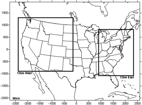
The CMAQ inputs for 2008 meteorology and boundary conditions, and 2008, 2020, and 2030 National Emissions Inventories, were based on existing data sets. Meteorological outputs from version 3 of the Weather Research and Forecasting (WRF) model (Skamarock et al., 2008) for the base year 2008 were obtained from the EPA for the eastern U.S. simulation and from the ongoing Western Regional Air Partnership West-wide Jumpstart Air Quality Modeling Study (WestJumpAQMS; http://www.wrapair2.org/WestJumpAQMS.aspx) for the CONUS (Continental US) and western U.S. simulations The emissions for the 2008 base year were based on the EPA 2008 National Emissions Inventory (NEI) version 1.5 (http://www.epa.gov/ttnchie1/net/2008inventory.html, accessed March 2013) released in May 2011. The emission inventory for the 2018 future year was based on the EPA inventory for 2020, projected from the 2005 NEI version 4 (http://www.epa.gov/ttn/chief/emch/index.html, accessed March 2013). The emission inventory for the 2030 future year was based on the EPA's 2030 emission inventory developed for the modeling analysis of the Heavy Duty Vehicle Green House Gas (HDGHG) regulation (EPA, 2011). The mobile source emissions in these future year inventories were further adjusted, as discussed later in this article, for the CMAQ modeling conducted in this study. The CMAQ simulations conducted for this study used a nested-grid configuration, with a 36 × 36-km resolution CONUS domain covering the lower 48 states and adjacent portions of Canada and Mexico, and two 12 × 12-km resolution inner domains covering the eastern U.S. and the western U.S. Figure 1 shows the three modeling domains, and the number of horizontal grid cells in each domain. The modeling domains extend vertically from the surface to the 100 mbar level (approximately 15 km) using a sigma-pressure coordinate system and 26 layers. Predictions from the outer coarse-resolution domain provided the initial and boundary conditions for the finer 12-km-grid resolution inner domains. Boundary conditions for the 36-km resolution CONUS domain were based on outputs from the global chemistry model Model of Ozone and Related Chemical Tracers (MOZART-4), driven by meteorological fields from the National Aeronautics and Space Administration (NASA) Global Modeling and Assimilation Office (GMAO) Goddard Earth Observing System (GEOS-5) model (http://www.acd.ucar.edu/wrf-chem/mozart.shtml).

Figure 1. The 36-km and western/eastern U.S. 12-km modeling domains for the CMAQ simulations. The CMAQ domain for the 36-km grid was 148 × 112, (−2736, −2088) to (2592, 1944), whereas the 12-km grid in the west was 186 × 183, (−2376, −900) to (−144, 1296), and the 12-km grid in the east was 119 × 158, (912, −1080) to (2340, 816).

Future year emissions

There were several existing future year emission projections that were leveraged to create the 2018 and 2030 future year emission inventories. These projections were based on decisions made about possible future changes in demand, technology, and regulation. Future changes in technology were based on current science and assumptions about future application and trends. Regulation impacts were estimated for regulations already OTB. However, for future year scenario projections beyond the immediate future, attempts were made to include OTW regulations. These OTW regulations were those that were not yet law, but were reasonably assumed to be in place by the projected date.

The mobile source emissions in the above inventories were updated by conducting mobile source modeling using the LEV III/Tier 3 light-duty vehicle emission inventories. In the emissions projections for base scenarios for 2018 and 2030, the federal, state, and local rules that would apply are shown in Table 1.

Table 1. Federal, state, and local rules for future year base scenarios

Rule	Reference
Tier 2 Rule	http://www.epa.gov/oms/standards/light-duty/tier2stds.htm
2007 On-road Heavy-Duty Rule	http://www.epa.gov/otaq/highway-diesel/regs/2007-heavy-duty-highway.htm
Mobile Source Air Toxics Rule (MSAT2)	http://www.gpo.gov/fdsys/pkg/FR-2007-02-26/html/E7-2667.htm
Clean School Bus USA Program	http://www.epa.gov/reg3artd/vehicletran/vehicles/schoolbus.htm
Renewable Fuel Standard	http://www.epa.gov/otaq/fuels/renewablefuels/index.htm
National Low Emission Vehicle Program (NLEV)	http://www.epa.gov/oms/lev-nlev.htm
Ozone Transport Commission (OTC) LEV Program	http://www.gpo.gov/fdsys/pkg/FR-1995-01-24/html/95-1387.htm
State of California LEV II rules	http://www.arb.ca.gov/msprog/levprog/levii/levii.htm

On-road mobile source emission projections were created through the use of two different mobile source models. Emissions for the state of California were projected with the Emissions Factor 2007 (EMFAC2007) (CARB, 2006) model, whereas emissions for the rest of the U.S. were projected with the Motor Vehicle Emissions Simulator (version: MOVES2010a) model (EPA, 2010). The projections generated by both models were based on changes expected due to implementation of regulations as well as growth projections.

For the future year sensitivity scenarios, the light-duty portions of the LEV III and expected Tier 3 rules were included in the emissions projections. The standards for these two rules were simulated as being similar, differing only in implementation schedule and location. LEV III applies only to the state of California vehicles, whereas Tier 3 was applied to the rest of the U.S. Thus, the new regulations were accounted for in the 2030 projections.

The LEV III and Tier 3 regulations include three parts: the super ultra-low-emission vehicle (SULEV) exhaust requirement, the second version of the Supplemental Federal Test Procedure (SFTP 2) exhaust requirement, and the evaporative emissions requirement. These regulations apply to new model year vehicles. Table 2 shows the implementation timing for the LEV III and Tier 3 rule segments. Within EMFAC, the SULEV portion of the standard was modeled by setting an increasing percentage of the light-duty vehicle fleet to the advanced technology partial zero emission vehicle (AT-PZEV) vehicle type each year from 2015 through 2025. The SULEV component of the LEV III/Tier 3 Standard requires a gradual phase-in of vehicles that meet the California SULEV requirements until all of the new light-duty vehicle fleet meets the SULEV standard. This will lead to reductions in emissions of hydrocarbons (HC), carbon monoxide (CO), and nitrogen oxides (NO_x). In both the LEV III and Tier3 standards, the phase-in is complete by calendar year 2025. Within MOVES, the SULEV portion of the standard was modeled by scaling the MOVES LEV II emission factors. These scaling factors are provided in Table 3.

Table 2. Phase-in (%) schedule simulated for LEV III and Tier 3

	SULEV and SFTP		Zero Evaporative
Year	LEV III	Tier 3	LEV III and Tier 3
2015	9	0
2016	18	0
2017	27	11	40
2018	36	22	60
2019	45	33	80
2020	55	44	100
2021	64	55
2022	73	66
2023	82	77
2024	91	88
2025	100	100

Table 3. Ratios used for the emissions standards for light-duty cars and trucks

LEV III/LEV II Ratio	HC	CO	NOx
Light-duty cars	0.242	0.532	0.568
Light-duty trucks	0.200	0.594	0.534

The second part of the LEVIII/Tier 3 standard is the Evaporative Standard. It requires that upon full implementation, all light-duty vehicles have zero fuel-related evaporative emissions. The phase-in for this portion of the regulation is the same for both California and the rest of the country. The evaporative standard is projected to begin phase-in in 2017 and will be completely phased-in by 2022. Within EMFAC, the evaporative standard was implemented by setting the appropriate fraction of light-duty vehicles in each model year to the vehicle evaporative technology representing zero fuel-based evaporative emissions. Within MOVES, the evaporative standard was implemented through the use of the MOVES zero emission vehicle (ZEV) tool. The ZEV tool sets a user-specified percentage of the fleet to meet the zero fuel-based evaporative standards for each vehicle model year.

The third and final part of the standard is the SFTP 2 or Aggressive Driving Standard. Specifically, it represents the impact of high-speed/high-load driving referred to as US06 and the use of vehicle air conditioners, referred to as SC03. The current SFTP standard applies to the first 4000 miles, whereas the new SFTP standard applies up to 150,000 miles. The SFTP 2 standards are applied starting in 2015 and full compliance is reached by 2025. To translate these test-based standards into an emission inventory, a weighting scheme is needed to apportion the time or miles corresponding to various normal and aggressive conditions. Equation 1 used was to determine the weighted emissions:

1

The SFTP 2 standard cannot be modeled directly by the EMFAC model. Instead, the results of the LEV III scenario were run through a mathematical routine to calculate projected emissions reductions due to the SFTP 2 standard. The projected impact of the SFTP 2 standard were calculated using a ratio of the emissions allowed under the original SFTP standard (it was assumed that emissions calculated by EMFAC account for the original SFTP standard) with the emissions allowed under the SFTP 2 standard. This method was expected to overpredict the impact of SFTP 2, as some current vehicles meet the SFTP 2 standards without modifications. Additionally, although the standard only applies up to 150,000 miles, it was not possible to restrict the application of the standard due to mileage, so this limit was not modeled. Finally, SFTP 2 limits the emissions of the sum of NMHC and NO_x emissions rather than limiting them separately as the SULEV standard does. Because the sum of NO_x and NMHC reduction form is unknown, the emissions reduction was taken half from NO_x and half from NMHC. Additionally, the MOVES model cannot directly model the SFTP 2 Standard. Instead, ratios of SFTP/SFTP 2 as calculated above for California were calculated for the national scale. Whereas EMFAC differentiates between the results for different exhaust emissions categories and vehicle model years, MOVES provides differentiation only by fuel type and vehicle category. Therefore, one ratio per vehicle category needed to be calculated and applied to the entire light-duty vehicle fleet for each calendar year. Although the estimation methods of EMFAC and MOVES are quite different, this approach for California was used to calculate the impact of SFTP 2 on the phased-in new SULEV vehicle fleet following the Tier 3 phase-in schedule. The ratios, provided in Table 4, were then applied to the emission factors for MOVES. This method produced a ratio of 1 for 2018 due to very limited market penetration and the small impact of the reduction on new vehicles. Although the impact on emissions in 2025 and 2030 was larger than in 2018, it was a 3% reduction for HC + NO_x.

Table 4. Ratios to reduce emission factors due to SFTP 2

Inventory Year	HC and NOx Factor
2018	1
2025	0.993
2030	0.972

Tables 5 and 6 show the future year baseline and LEV III/Tier 3 average daily light-duty vehicle emissions in tons per day in California and the rest of the U.S., respectively. The LEV III and Tier 3 standards have little impact in 2018 because the regulations are just beginning to be phased in. By 2030, when the regulations have been phased in to impact 100% of the new light-duty vehicle fleet, the amount of emissions reductions between baseline and the revised standard increase. The vehicles in the California fleet begin with fewer emissions than vehicles in the U.S. fleet. So, as time progresses, the U.S. fleet replaces the higher emission vehicles with less emission vehicles. This results in greater percentage emission reductions in 2030 in the U.S. fleet than in the California fleet.

Table 5. California summer light-duty vehicle emissions (tons per day)

Pollutant	Baseline (LEV II)	LEVIII	% Change (LEV II versus LEV III)
2018
VOC	248	248	−0.2%
CO	1868	1855	−0.7%
NOx	153	152	−0.4%
2030
VOC	164	156	−4.9%
CO	1090	946	−13.2%
NOx	77	69	−10.6%

Table 6. U.S. summer light-duty vehicle emissions (tons per day)

Pollutant	Baseline (Tier 2)	Tier 3	% Change (Tier 2 versus Tier 3)
2018
VOC	2680	2661	−0.7%
CO	38733	38589	−0.4%
NOx	3911	3905	−0.2%
2030
VOC	1897	1094	−42.3%
CO	35898	28244	−21.3%
NOx	2201	1845	−16.2%

Results and Discussion

Model performance

The base year simulation results were used to evaluate CMAQ model performance for July 2008. An operational model performance evaluation (MPE) was performed in which CMAQ estimates of ozone concentrations for the simulation period were compared with observed values. The procedures and equations for the MPE are based on guidance from the EPA (EPA, 1991, 2001, 2007). CMAQ was evaluated for both the eastern and western U.S. 12-km domains, using ozone observations from the Air Quality System (AQS) monitoring network. Table 7 provides detailed model performance statistics for CMAQ ozone estimates and shows that the bias and error in model estimates generally meet the EPA recommended goals for ozone performance.

Table 7. Model performance statistics for hourly ozone concentrations for July 2008

Performance	12 km West	12 km East
Fractional bias (%)	−10	−17
Fractional gross error (%)	26	31
Paired peak accuracy (%)	3	17
Normalized mean bias (%)	−6	−12
Normalized mean error (%)	24	27
Mean normalized bias (%)	−5	−10
Mean normalized gross error (%)	24	27
Mean bias (ppb)	−4	−7
Mean absolute gross error (ppb)	13	15
Observed maximum (ppb)	150	128
Predicted maximum (ppb)	154	150
Observed arithmetic mean (ppb)	56	56
Predicted arithmetic mean (ppb)	52	49
R ^2	0.17	0.03
Number of data points	59,953	66,300
Note: These statistics are calculated only for those observed concentrations where 1-hr O3 ≥40 ppb.

The statistics are calculated only for those observed concentrations where 1-hr O₃ ≥40 ppb. The model performs better in the western U.S. than in the eastern U.S. In the western U.S. domain, the fractional bias (−10%) and fractional error (26%) metrics are within EPA's performance goals (≤±15% and ≤35%, respectively). The model performance in the eastern U.S. domain has a fractional bias (−17%) slightly worse than the EPA performance goal, and a fractional error (31%) within the EPA guideline. For both modeling domains, the model tends to underpredict observed ozone concentrations. The correlation between observed and predicted O₃ concentrations is low, particularly in the eastern U.S., as shown by the R ² of 0.17 and 0.03 for the western and eastern U.S., respectively. One major difference between the western and eastern U.S. simulation is the source of the meteorology inputs.

Future year results

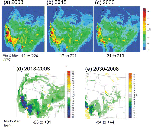
Figure 2 shows the CMAQ 12-km resolution western U.S. domain daily maximum 8-hr ozone concentrations for the 2008 base year, 2018, and 2030 for July 7, when the maximum 8-hr average ozone in the base year simulation was about 225 ppb. The results for other days in July, as well as monthly maximum 8-hr average ozone concentrations in the western U.S. domain, are qualitatively similar to those for July 7. Figure 2 also shows the July 7 differences between the base year and each of the future years. The future year July 7 simulations were performed with the mobile source LEV III/Tier 3 updates discussed previously. The future year changes to the 8-hr average ozone maximum concentration decrease from 2008 by 3 ppb in 2018 and 5 ppb in 2030. There are large decreases from 2008 over most of the domain, with maximum decreases of 23 ppb in 2018, and 34 ppb in 2030. There are also a few areas where an increase in 8-hr average ozone concentration is predicted. The maximum increase, in the Southern California Air Basin (SoCAB), ranges from 31 ppb in 2018 to 44 ppb in 2030. Specifically, there are large areas with decreases in 8-hr average ozone concentrations, and smaller areas with small increases. Thus, the future year scenarios show a fairly significant improvement in ozone concentrations over much of the modeling domain. Projected ozone increases in some areas and decreases in other areas are a result of emission changes, meteorology, and photochemistry. When VOC levels are high relative to NO_x, in areas with large biogenic VOC emissions, ozone is reduced by NO_x reductions and increased by NO_x increases. Such conditions are called “NO_x-limited” or “NO_x-sensitive.” However, when NO_x levels are relatively high and VOC levels are relatively low, increases in NO_x can decrease ozone, because NO reacts directly with ozone and NO₂ terminates radicals, forming nitric acid, which is removed from the system or forms particulate nitrates. Such conditions are called “VOC-limited,” “VOC-sensitive,” or “NO_x-saturated.” Under these conditions, VOC reductions are effective in reducing ozone, but NO_x reductions can increase ozone under certain circumstances. Hence, decreasing NO_x more than decreasing VOC results in ozone increases (Cook et al., 2010). The ozone increase predicted in the western portion of the SoCAB is because the area is likely VOC-sensitive and is projected to experience NO_x decreases.

Figure 2. Western U.S. daily maximum 8-hr ozone on July 7 in (a) 2008, (b) 2018, and (c) 2030. For comparison, the change in ozone is shown for July 7 between (d) 2018 and 2008 and (e) 2030 and 2008.

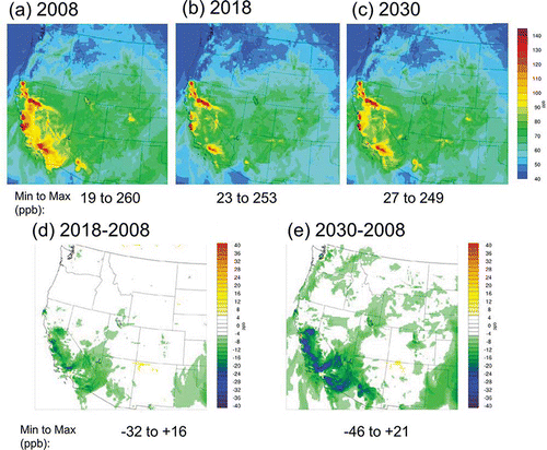
The July maximum 8-hr average ozone concentrations in the western U.S. domain are shown in Figure 3 for the base year simulation and two future year simulations along with the differences between the base and future years. The differences are qualitatively similar to the differences for July 7 discussed previously. For the most part, there are large areas with large decreases in 8-hr average ozone concentrations, and smaller areas with small increases. Thus, the western U.S. in the month of July for future year scenarios predicts a fairly significant improvement in ozone concentrations over much of the modeling domain.

Figure 3. Western U.S. spatial plots of July maximum 8-hr ozone concentrations for (a) 2008, (b) 2018, and (c) 2030. For comparison, the change in ozone is shown for July between (d) 2018 and 2008 and (e) 2030 and 2008.

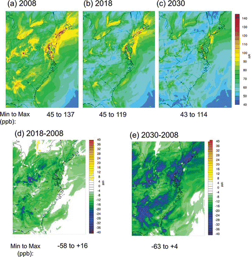
Figure 4 shows the July 17 corresponding 8-hr average ozone concentration results for the eastern U.S. domain along with the differences for July 17 in future years. The July 17 eastern U.S. domain maximum 8-hr average ozone concentrations are qualitatively similar to predicted results for July 17 in future years, as well as for other days in July. Figure 5 shows the maximum July 8-hr average concentration results and the difference between base and future years. As compared with the western U.S. results, there are large decreases in ozone concentrations throughout the domain with isolated pockets of small increases. The maximum decreases in the eastern domain compared to 2008 are 58 ppb in 2018 and 63 ppb in 2030. The maximum increases from the base year values were about 6 ppb in both 2018 and 2030.

Figure 4. Eastern U.S. daily maximum 8-hr ozone on July 17 in (a) 2008, (b) 2018, and (c) 2030. For comparison, the change in ozone is shown on July 17 between (d) 2018 and 2008 and (e) 2030 and 2008.

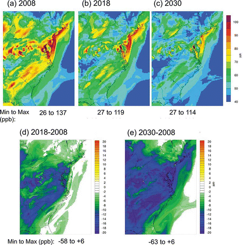
Figure 5. Eastern U.S. spatial plots of July maximum 8-hr ozone concentrations for (a) 2008, (b) 2018, and (c) 2030. For comparison, the change in ozone is shown for July between (d) 2018 and 2008 and (e) 2030 and 2008.

Conclusion

Changes in future year ozone concentrations in the eastern and western U.S. for a summer month were simulated using CMAQ version 4.7.1. Existing future year inventories were updated to include expected future emission regulations, which are OTB and OTW for on-road mobile, nonroad mobile, point, and area source emissions. The modeling results showed general decreases in ozone in future years over most of the modeling domain, although there were also some increases in ozone in certain areas. In the western U.S., some increase in 8-hr ozone was predicted in the Los Angeles area. There are areas where more than 75 ppb of 8-hr ozone remain in California in 2030. The minimum value of the 8-hr maximum ozone concentration in the western region increased by about 8 ppb in 2030. In the eastern U.S., in 2030, all areas show improvement in the 8-hr ozone concentration, except for small increases in isolated pockets. However, areas with 8-hr ozone over 75 ppb in the Northeast are still predicted to occur. The minimum value of the 8-hr maximum ozone concentration in the eastern U.S. essentially does not change.

This study provides an understanding of expected changes in future year ozone concentrations due to projected changes in emissions. Future studies will investigate the contributions of different anthropogenic source categories, natural emissions, and global background concentrations to these estimates. These source attribution studies will provide a better understanding of the benefits of reductions in emissions from the different anthropogenic source categories, as well as an understanding of the limits on the benefits imposed by natural sources and the global background.

References

- Byun , D. and Schere , K.L. 2006 . Review of the governing equations, computational algorithms, and other components of the Models-3 Community Multiscale Air Quality (CMAQ) modeling system . Appl. Mech. Rev , 59 : 51 – 77 . doi: 10.1115/1.2128636
- California Air Resources Board. 2006. EMFAC2007 User's Guide, November 2006 http://www.arb.ca.gov/msei/onroad/downloads/docs/user_guide_emfac2007.pdf (http://www.arb.ca.gov/msei/onroad/downloads/docs/user_guide_emfac2007.pdf) (Accessed: 4 March 2013 ).
- Collet , S. , Kidokoro , T. , Sonoda , Y. , Lohman , K. , Karamchandani , P. , Chen , S.-Y. and Minoura , H. 2012 . Air quality impacts of motor vehicle emissions in the south coast air basin: Current versus more stringent control scenario . Atmos. Environ , 47 : 236 – 240 . doi: 10.1016/j.atmosenv. 2011.11.010
- Cook , R. 2010 . Air quality impacts of increased use of ethanol under the United States’ energy Independence and Security Act . Atmos. Environ , 45 : 7714 – 7724 . doi: 10.1016/j.atmosenv.2010.08.043
- ENVIRON. 2011. User's Guide, Comprehensive Air Quality Model with Extensions (CAMx), version 5.40, 2011 http://www.camx.com/files/camxusersguide_v5-40.aspx (http://www.camx.com/files/camxusersguide_v5-40.aspx) (Accessed: 1 April 2013 ).
- Koffi , B. , Szopa , S. , Cozic , A. , Hauglustaine , D. and van Velthoven , P. 2010 . Present and future impact of aircraft, road traffic and shipping emissions on global tropospheric ozone . Atmos. Chem. Phys , 10 : 11681 – 11705 . doi: 10.5194/acp-10-11681-2010
- Matthes , S. , Grewe , V. , Sausen , R. and Roelofs , G.J. 2007 . Global impact of road traffic emissions on tropospheric ozone . Atmos. Chem. Phys , 7 : 1707 – 1718 . doi: 10.5194/acp-7-1707-2007
- Nopmongcol , U. , Griffin , W.M. , Yarwood , G. , Dunker , A.M. , Maclean , H.L. , Mansell , G. and Grant , J. Impact of dedicated E85 vehicle use on ozone and particulate matter in the U.S . Atmos. Environ , 45 7330 – 7340 .
- Roustan , Y. , Pausader , M. and Seigneur , C. Estimating the effect of on-road vehicle emission controls on future air quality in Paris, France . Atmos. Environ , 45 6828 – 6836 . doi: 10.1016/j.atmosenv.2010.10.010
- Skamarock , W.C. , Klemp , J.B. , Dudhia , J. , Gill , D.O. , Barker , D.M. , Duda , M.G. , Huang , X.-Y. , Wang , W. and Powers , J.G. 2008 . A Description of the Advanced Research WRF Version 3 , Boulder , CO : Mesoscale and Microscale Meteorology Division, National Center for Atmospheric Research . NCAR Techical Note NCAR/TN-475+STRJune 2008
- U.S. Environmental Protection Agency . 1991 . Guidance for Regulatory Application of the Urban Airshed Model (UAM) , Research Triangle Park , NC : Office of Air Quality Planning and Standards, U.S. Environmental Protection Agency .
- U.S. Environmental Protection Agency. 1999. Technical Support Document for the Tier 2/Gasoline Sulfur Ozone Modeling Analyses. EPA420-R-99-031. Research Triangle Park, NC: Office of Air Quality Planning and Standards, U.S. Environmental Protection Agency; December 1999 http://www.epa.gov/tier2/documents/r99023.pdf (http://www.epa.gov/tier2/documents/r99023.pdf) (Accessed: 1 August 2014 ).
- U.S. Environmental Protection Agency . 2001 . Guidance for Demonstrating Attainment of Air Quality Goals for PM2.5 and Regional Haze. Draft report , Research Triangle Park , NC : U.S. Environmental Protection Agency .
- U.S. Environmental Protection Agency . 2007 . Guidance on the Use of Models and Other Analyses for Demonstrating Attainment of Air Quality Goals for Ozone, PM2.5 and Regional Haze , Research Triangle Park , NC : U.S. Environmental Protection Agency . EPA-454/B-07-002
- U.S. Environmental Protection Agency . 2010 . User Guide for MOVES2010a , Research Triangle Park , NC : Office of Transportation and Air Quality, U.S. Environmental Protection Agency . EPA-420-B-10-036August 2010
- U.S. Environmental Protection Agency . 2011 . Heavy-Duty Vehicle Greenhouse Gas (HDGHG) Emissions Inventory for Air Quality Modeling Technical Support Document , Research Triangle Park , NC : Office of Air and Radiation, U.S. Environmental Protection Agency .
- Vijayaraghavan , K. , Yarwood , G. , Lindhjem , C. , DenBleyker , A. , Nopmongcol , U. , Grant , J. , Tai , E. , Sakulyanontvittaya , T. and Johnson , J. 2012 . Estimating the effect of past, present and potential future emission standards for light duty gasoline vehicles on ozone and fine particulate matter in the eastern United States . Atmos. Environ , 60 : 109 – 120 . doi: 10.1016/j.atmosenv.2012.05.049