Impact of emissions from natural gas production facilities on ambient air quality in the Barnett Shale area: A pilot study

Abstract

Rapid and extensive development of shale gas resources in the Barnett Shale region of Texas in recent years has created concerns about potential environmental impacts on water and air quality. The purpose of this study was to provide a better understanding of the potential contributions of emissions from gas production operations to population exposure to air toxics in the Barnett Shale region. This goal was approached using a combination of chemical characterization of the volatile organic compound (VOC) emissions from active wells, saturation monitoring for gaseous and particulate pollutants in a residential community located near active gas/oil extraction and processing facilities, source apportionment of VOCs measured in the community using the Chemical Mass Balance (CMB) receptor model, and direct measurements of the pollutant gradient downwind of a gas well with high VOC emissions. Overall, the study results indicate that air quality impacts due to individual gas wells and compressor stations are not likely to be discernible beyond a distance of approximately 100 m in the downwind direction. However, source apportionment results indicate a significant contribution to regional VOCs from gas production sources, particularly for lower-molecular-weight alkanes (<C6). Although measured ambient VOC concentrations were well below health-based safe exposure levels, the existence of urban-level mean concentrations of benzene and other mobile source air toxics combined with soot to total carbon ratios that were high for an area with little residential or commercial development may be indicative of the impact of increased heavy-duty vehicle traffic related to gas production

Implications

Rapid and extensive development of shale gas resources in recent years has created concerns about potential environmental impacts on water and air quality. This study focused on directly measuring the ambient air pollutant levels occurring at residential properties located near natural gas extraction and processing facilities, and estimating the relative contributions from gas production and motor vehicle emissions to ambient VOC concentrations. Although only a small-scale case study, the results may be useful for guidance in planning future ambient air quality studies and human exposure estimates in areas of intensive shale gas production.

Introduction

The Barnett Shale is a geological formation that stretches from Dallas to west of Fort Worth and southward (Texas), covering at least 5000 square miles and 18 counties in the Fort Worth Basin. It is one of the largest onshore natural gas fields in the United States, containing not only natural gas but also condensate and light oil. With advances in horizontal drilling and hydraulic fracturing techniques, the number of producing gas wells in the United States increased by 50% between 2000 and 2011 (U.S. Energy Information Administration, 2013), reaching 514,637. In the Barnett Shale area, the number of shale gas wells increased from 726 in 2000 to nearly 15,000 by December 2010 (Texas Railroad Commission, 2013). This surge in exploration and production has been accompanied by public concerns regarding environmental issues, including air quality, water quantity and quality, and human health impacts (Jackson et al., 2013; Krzyzanowski, 2012; McKenzie et al., 2012, 2014; Warner et al., 2012).

According to Branosky et al. (2012), there are five stages of the natural gas life cycle: (1) preproduction; (2) natural gas production; (3) natural gas transmission, storage, and distribution; (4) natural gas end-use; and (5) end-of-well production life. Emissions of methane and other compounds from activities in the first two of the five natural gas life cycle stages can impact local and regional air quality. The preproduction stage includes everything from exploration, site clearing, and road construction to drilling, hydraulic fracturing, and well completion. For a single well, preproduction is usually completed within a few weeks; however, these operations may be carried out for a dozen or more wells on a pad and at multiple sites in the field, lasting for months. A recent review (Moore et al., 2014) discusses the emissions from this stage in more detail.

The natural gas production stage may continue for many years, depending on the site. The natural gas that flows directly from the well often contains other associated nonmethane hydrocarbons (NMHCs), water vapor, carbon dioxide, hydrogen sulfide, or natural gas liquids in various proportions and needs processing to meet purity standards for addition to the pipeline infrastructure, known as “pipeline quality” (>90% methane). Processing occurs near the well or at a centralized processing plant. Emission sources include well-head compressors or pumps that bring the produced gas up to the surface or up to pipeline pressure (engines are often fired with raw or processed natural gas), compressor stations, oil and condensate tank venting, production well fugitives, dehydrator generation venting, venting from pneumatic pumps and devices that are actuated by natural gas, leaks through faulty casing, incomplete emission capture, or burning in flaring systems. These emissions can be continuous or intermittent but will be on-going during the entire lifetime of the well (Moore et al., 2014). In addition, emissions from the diesel engine–powered trucks that service the wells and compressor stations may also be important. A compilation of emission data from natural gas production in the Barnett Shale area (Armendariz, 2009) concluded that condensate tank venting was the largest single source of volatile organic compounds (VOCs) from the natural gas production. In contrast, a separate study commissioned by the City of Fort Worth (Eastern Research Group, 2011) in which emission measurements were made at 375 wells and 8 compressor stations estimated that 60% of the total hazardous air pollutants (HAPs) and 56% of VOCs emitted by natural gas production activity in the Fort Worth area was from compressor stations and 30% of HAPs (35% of VOCs) from well pads. However, the majority of wells in the Fort Worth metro area are classified as dry gas (low condensate production) and drilling/fracking operations were not included in this estimate, so the results may not be representative of the larger Barnett Shale area. The Fort Worth Study (Eastern Research Group, 2011) did observe that the largest source of fugitive emissions that could be detected with an infrared (IR) camera was leaking tank “thief hatches” (pressurized caps on access ports for sampling tank contents). Malfunctioning pneumatic controllers on separator valves were also identified as a common source of fugitive gas emissions.

Several recent studies addressed the impact of natural gas development and production on air quality (Moore et al., 2014). However, only a few studies addressed the problem of air toxics that could be attributed to unconventional natural gas exploration and production, and the conclusions ranged from significant (McKenzie et al., 2012, 2014) to little or no impact at all (Bunch et al., 2014). Bunch et al. (2014) evaluated more than 4.6 million of measurements, representing data from seven VOC monitors established by the Texas Commission on Environmental Quality (TCEQ) in the Barnett Shale area. Measured air concentrations were compared with federal and state health-based air comparison values (HBACVs) to assess potential acute and chronic health effects. They found that none of the measured VOC concentrations exceeded applicable acute HBACVs. Similarly, measured and estimated air pollution levels from the Fort Worth Study (Eastern Research Group, 2011) did not exceed those known to cause adverse health effects. Further, the measured benzene and formaldehyde levels were not unusually elevated when compared with levels currently measured by TCEQ elsewhere in Texas.

McKenzie et al. (2012) conducted a preliminary health impact assessment study in rural Garfield County, Colorado, and reported that public health most likely would be impacted by well completion activities (when emissions are the highest), particularly for residents living nearest the wells (within 0.5 mile). More recently, McKenzie et al. (2014) conducted a retrospective cohort study to investigate the association between density and proximity of natural gas wells to maternal residences in rural Colorado and three classes of birth defects. Their study suggests a positive association between greater density and proximity of natural gas wells within a 10-mile radius of maternal residence and greater prevalence of congenital heart defects and possibly neural tube defects.

In 2009, very limited data were available regarding the air quality impacts of unconventional natural gas development in the Barnett Shale formation. Recognizing the need for additional data on emissions from natural gas production facilities in the Barnett Shale area and their potential impact on population exposures, the Mickey Leland National Urban Air Toxics Research Center funded a short-term (7 months) focused study reported on here (see also Zielinska et al., 2011). Results were expected to help lead to a better understanding of toxic air emissions in this area and the potential for exposure of residents. The major objectives of this preliminary study were (1) characterize the chemical composition of emissions related to natural gas production operations in the Barnett Shale area; (2) estimate the potential emission impacts from various types of natural gas production facilities by measuring the associated pollutant gradients from the point of emissions; and (3) determine the ambient concentrations of selected air toxics within a community in the Barnett Shale region, and, to the extent possible, apportion the contributions of emissions from gas production operations to the measured exposure concentrations.

These objectives were addressed in two phases: in the first phase of this study, an initial survey was performed using a mobile sampling vehicle to identify facilities with measurable emissions. Source-oriented samples were then collected at several facilities where elevated concentrations were measured by continuous survey monitors. Continuous measurements were also made at various locations near the facilities to characterize the spatial variations in pollutant concentrations. In Phase 2, saturation monitoring (multiple fixed ambient sampling locations) was conducted at residential locations adjacent to gas production areas. One location was near a well with emissions from condensate tanks that were well characterized during Phase 1. A single private residence was located a short distance downwind of this well and away from other emission sources that might interfere with the measured gradient of emissions from the well. The measurement at this site served as a case study of the extent of pollutant gradients from a well-characterized emission source relative to the upwind pollutant concentrations. The second facility was a gas compressor station located near a small community. The spatial variations in pollutant concentrations were measured at various distances and directions from the source, including sites adjacent to nearby roadways and a background site located upwind of the community. The measured VOCs were apportioned to sources using the Chemical Mass Balance receptor model. The study results were placed in context by comparing the measured pollutant concentrations with comparable data from elsewhere in the Barnett Shale area and from urban areas of Dallas-Fort Worth.

Experimental Methods

Phase 1—Sample collection for characterization of emission sources

Phase 1 of the study was conducted from April 15 to 23, 2010, and included mobile sampling with continuous monitors to select appropriate emission sources for monitoring and time-integrated (over 1 hr) sampling of VOCs and related air pollutants at selected facilities to determine chemical source profiles.

Wise County was chosen for the monitoring area because it has a high density of active wells and the wells produce significant quantities of condensate (Texas Railroad Commission, 2010). Natural gas condensate contains aromatic and higher-molecular-weight (MW) aliphatic hydrocarbons. The aforementioned Fort Worth Study (Eastern Research Group, 2011) found little difference in average total organic carbon (TOC) emissions between dry and wet gas sites, but average VOC and HAP emissions from wet gas sites proved to be considerably higher.

The selection of the gas production facilities for monitoring was based on surveying candidate sites using a mobile monitoring system equipped with several continuous monitors described in the Sampling and Analytical Methods section. Approximately two dozen well sites were surveyed in the areas surrounding Rhome, Decatur, Aurora, Boyd, New Fairview, Alvord, Bridgeport, Runaway Bay, Chico, Paradise, and Allison. Measurements were also made near the fencelines of gas compression/processing plants near Rhome, Chico, Bridgeport, Allison, and New Fairview. Although there were several hydraulic fracturing operations conducted in the area, we were unable to get closer than 200–300 m from the drill pads, and access to downwind locations was unavailable during that time.

Based on the mobile surveys, seven locations were chosen for collection of source samples to be analyzed for chemical speciation. Source samples included canister samples for VOC characterization and 2,4-dinitrophenyl hydrazine (DNPH)-impregnated Sep-Pak cartridges for carbonyl compound collection. In general, 1-hr samples were collected with the exception of a few “grab samples” collected over a few minutes. Due to the large sample mass required for speciated particulate matter measurements, and the low probability of any significant emissions from producing gas wells, no particle filter samples were collected during Phase 1. A portable meteorology package was deployed to measure wind speed, wind direction, relative humidity, and temperature during sampling. Source samples were collected downwind of wells with condensate tanks releasing measurable quantities of VOCs, near large and small compressor stations, adjacent to the main highway in Decatur, along a rural country road with no nearby wells or residences, and at a private residence while a gasoline-powered lawnmower was being used. A complete list of the facilities selected for source sampling, the type of samples collected at each site, and the meteorological conditions during each sampling event is included in Supplemental Material (Table S1) along with a figure showing the location of the areas selected for monitoring (Figure S1).

Phase 2—Saturation monitoring and gradient measurements

During Phase 1 of the study, the Shale Creek community in Rhome was selected for ambient monitoring in Phase 2 of the study. The community of Shale Creek is located on 330 acres with over 1000 single-family home sites (http://www.shalecreekcommunity.com/community.html), adjacent to a large compressor station. At the time of this study, around 250–300 houses were occupied. The compressor station is near the southwest edge of Shale Creek and is screened from the community by a high sound wall. In addition, there are numerous production wells in the surrounding area. Measurements at these sites included 7-day average concentrations of oxides of nitrogen (NO_x), nitrogen dioxide (NO₂), sulfur dioxide (SO₂), speciated C5–C9 hydrocarbons, including n-alkanes, 1,3-butadiene, and BTEX (benzene, toluene, ethylbenzene, and xylenes), CS₂, and carbonyl compounds (formaldehyde, acetaldehyde, and acrolein) using passive samplers. Additionally, 7-day Teflon and quartz filter samples were collected with portable Airmetrics MiniVol samplers (Springfield, OR) at seven sites and analyzed for PM_2.5 mass (particulate matter with an aerodynamic diameter ≤2.5 μm), elements Na to U, organic carbon (OC) and elemental carbon (EC), and polycyclic aromatic hydrocarbons (PAHs). The sampling sites and the type of samples collected at each site are mapped in Figure 1.

Figure 1. Map of Shale Creek community sampling sites. Markers with black dots inside indicate sites with both passive (NO_x, SO₂, speciated VOCs) and active filter samplers. Other sites had only passive samplers.

A residential property in a rural community east of Decatur (Star Shell Road) was selected to measure the concentration gradient downwind of a known VOC source. This property is located near an active gas well with two condensate tanks that we had characterized during Phase 1. Three sets of passive NO_x, SO₂, and VOC samplers were installed at increasing distances from the condensate tanks (Figure 2): on a wooden fence surrounding the well pad (˜17 m from the tanks), on a barbed-wire fence surrounding the house (˜50 m from the first passive), and on the same fence further away from the source (˜30 m from the second site). All samplers were downwind from the source when the wind was from the prevailing southeast direction. One pair of filter samplers, with quartz and Teflon filters, was operated at the southeast corner of the residential property, downwind of the well. In addition, one set of passive samplers was installed along the south end of Star Shell Road, about 1 km upwind from the well and tanks to measure the regional background concentrations.

Figure 2. Star Shell Road source sample collection site: aerial view showing monitoring site locations. Symbols used are same as Figure 1.

Four sets of week-long time-integrated samples were collected at both Shale Creek and Star Shell Road, from April 22 to May 20, 2010. However, several sites, including critical background and near-source samples, were not included in the first week of sampling, so only results from the 21-day period beginning on April 29, 2010, are presented here (the partial data set covering the entire 4-week period did not indicate any substantial differences between the spatial pattern of concentrations during the first week and the rest of the study).

Sampling and analytical methods

Continuous methods

A compact 12-VDC monitor (2B Technologies model 400; Boulder, CO) that has sensitivity and resolution as low as 2 ppb was used for NO monitoring. A RAE Systems model PGM-7240 (ppbRAE; San Jose, CA) was used to continuously monitor ambient levels of VOCs that are detectable by photoionization detector (PID). This monitor responds to certain organic and inorganic gases that have an ionization potential of less than 10.6 eV, which includes aromatic hydrocarbons, olefins, and higher-molecular-weight alkanes. The PID monitor was calibrated in our laboratory using a standard mixture of hydrocarbons (BTEX and 1,3 butadiene). TSI DustTrak 8520 (Minneapolis, MN), a portable, battery-operated, laser-photometer that measures 90° light scattering and reports it as PM mass concentration, was used for the PM_2.5 mass monitoring. Additionally, an IR video camera sensitive to VOC absorption wavelengths (FLIR Systems Co. GasFindIR; Nashua, NH) became available on April 20, and was used to document gas leaks and other fugitive emissions. Wind speed and direction were also monitored during sample collection using Davis Instruments meteorology package (Hayward, CA).

Canister VOC sampling and analysis

Six-liter stainless steel Summa canisters (Restek, Bellefonte, PA) were cleaned prior to sampling by repeated evacuation and pressurization with humidified zero air, as described in the U.S. Environmental Protection Agency (EPA) document Technical Assistance Document for Sampling and Analysis of Ozone Precursors (October 1991; EPA/600-8-91/215). One canister out of the 10 per lot was filled with humidified ultra-high-purity (UHP) zero air and analyzed by the chromatography/mass spectrometry/flame ionization detector (GC/MS/FID) method, as described below. The canisters are considered clean if the target compound concentrations are less than 0.05 ppbv each. Canister samples were analyzed for BTEX, 1,3-butadiene, hexane, CS₂, and other VOC species according to EPA Method TO-15 (EPA, 1999b). See Supplemental Material for the list of species (Table S2) and detailed description of the analytical method.

DNPH cartridge samples for carbonyl compounds

Formaldehyde, acetaldehyde, and other carbonyl compounds (see Table S3 in Supplemental Material) were collected with Sep-Pak cartridges that have been impregnated with an acidified 2,4-dinitrophenylhydrazine (DNPH) reagent (Waters, Inc., Milford, MA), according to EPA Method TO-11A (EPA, 1999a). Carbonyls in the air sample are captured by reacting with DNPH to form hydrazones when the sample is drawn through the cartridge. Depending on the type of sorbent (C18, or silica gel) in the cartridge, the ambient measurement results are subject to various artifacts due to interaction with ozone (Tejada, 1986). To prevent this, the samplers in this study were equipped with potassium iodide (KI) denuder, as recommended in Method TO-11A. After sampling, the cartridges were eluted with acetonitrile and analyzed by a high-performance liquid chromatograph (Waters 2690 Alliance HPLC system with 996 photodiode array detector) using Polaris C18-A 3-μm 100 × 2.0 mm HPLC column. To correct for the acrolein rearrangement products (Tejada, 1986), a postanalysis reprocessing of the HPLC spectra was used, as described before (Fujita et al., 2011).

Passive sampling

Five different types of passive samplers were used, each with a unique adsorbent and method of analysis as listed in Table 1. After sampling, the collected pollutant was desorbed from the sampling medium by thermal or chemical means and analyzed quantitatively. The average concentration of the pollutant in the air to which the sampler was exposed can be calculated from the following relationship:

Table 1. Passive sampler types used for saturation monitoring

Manufacturer	Medium Type	Target Pollutants	Analysis Method
Ogawa	PS-124/134	NO2/NOx	Colorimetry for nitrite
Ogawa	PS-144	SO2	Ion chromatography
Radiello	141	HCs C4–C5, CS2	Thermal desorption/GC/MS
Radiello	145	HCs C6–C8	Thermal desorption/GC/MS
Radiello	165	Aldehydes	HPLC/UV

1

The sampling rate for every analyte was calculated experimentally, since pumps were not used in passive collection. Radiello (http://www.radiello.com) and Ogawa and Company (http://www.ogawausa.com/) supply these sampling rates for a number of commonly collected compounds. These sampling rates have been validated in chamber experiments for NO_x, formaldehyde, acrolein, BTEX, and SO₂ (Fujita et al., 2009; Mason et al., 2011). The sampling rates for pentane and isopentane were not available from Radiello and were determined experimentally in our laboratory, as described in Supplemental Material. Mass of analyte was calculated after the average blank result was subtracted from the analytical result. Sampling time is the amount of time that the sampler was exposed. Although lengthening the exposure time corresponds to an increase in sensitivity, it should be noted that exposure time is generally limited to 14 days due to the capacity of the adsorbents. Samples were analyzed in the Desert Research Institute (DRI) laboratory by thermal desorption GC/MS for VOCs, HPLC method as described for carbonyl compounds (EPA Method TO-11A), and by colorimetric methods (for passive Ogawa samples) according to the manufacturer’s specification. Details of the analytical methods and validation of sampling rates are described in Supplemental Material.

Time-integrated particle samples

Portable PM_2.5 air samplers from AirMetrics Corporation (Springfield, OR) were used for particle sampling for 7 continuous days (see Figure 1). The sampler is equipped with an inlet containing an impactor unit with 2.5-μm particle cut point and a flow control system capable of maintaining a constant flow rate (5 L/min). Particles were collected on Teflon filters (Gelman, Ann Arbor, MI; 47 mm Teflon filters) and prefired quartz 47 mm filters (Pallflex, Putnam, CT) that were analyzed gravimetrically for mass and by thermal/optical reflectance (TOR) for organic and elemental carbon (OC and EC), respectively (Chow et al., 1993). In addition, Teflon filters were analyzed for elements Na to U using energy-dispersive X-ray fluorescence (Watson et al., 1999). The details of these analyses are described in Supplemental Material.

After taking a punch for TOR analysis, quartz filters were spiked with the deuterated internal standards, extracted with dichloromethane utilizing pressurized fluid extraction method with accelerated solvent extractor (Dionex Corporation, Sunnyvale, CA) and analyzed for PAHs using the Varian 1200 triple quadrupole gas chromatograph/mass spectrometer (GC/MS/MS) system with CP-8400 autosampler (Varian, Inc., Walnut Creek, CA), operating in electron ionization (EI) and multiple ion detection (MID) mode. See Supplemental Material for more detailed description of analytical methods and the list of PAHs analyzed for this study. Quality assurance and data validation are also described there.

VOC source apportionment

The Chemical Mass Balance (CMB) receptor model (Watson et al., 1997) was applied in this study to apportion the source contributions to VOC concentrations in the Barnett Shale area. Version 8 of the DRI/EPA CMB receptor model was used to apportion hydrocarbon compounds to several source categories (motor vehicle exhaust, 2-stroke gas engine exhaust, natural gas, and condensate tank emissions). Source profiles were derived from the VOC canister samples collected during Phase 1 of this study and augmented with additional profiles prepared by DRI for other projects. Profiles created specifically for the study area were (1) a composite of two samples from the venting condensate tank at Star Shell Road; (2) a composite of fugitive emissions from two condensate tanks with open “thief hatches” (condensate tanks 3 and 4 in Table S1); (3) a mixed on-road motor vehicle exhaust profile based on the sample collected along I-287 in Decatur; and (4) a profile for small gasoline engines (Gas Lawnmower sample). We also attempted to create profiles representing downwind emissions from gas compression plants, but the canister samples collected from these locations proved to be too dilute to distinguish from the regional background. A variety of profiles from prior studies representing gasoline and diesel engine vehicle exhaust, fugitive and combustion emissions from natural gas operations, and biogenic sources were evaluated until a default set of chemical profiles (Table 2) were selected based upon best CMB model performance among the alternative source profiles. The source composition profiles were normalized to the sum identified species reported in Table S5, and composite profiles were derived by averaging the normalized fractions to give equal weight to all members of the composite. The uncertainties were set to the larger of the analytical uncertainties or 1σ variability in species abundances among members of a composite.

Table 2. VOC source profiles used for CMB receptor modeling

Profile Name	Emission Source Represented	Origin
TANK_VENT	Condensate tank fugitive emissions	Phase 1 of this project
NG	Residential natural gas	1998 Central Texas On-Road Hydrocarbon Study^a
LDGV	Light-duty gasoline vehicle exhaust	NREL/DOE Van Nuys Tunnel Study—Los Angeles, 2010^b
HDD	Heavy-duty diesel exhaust	EC Diesel Study^c
HWY_MIXED	Mixed-fleet highway emissions	Phase 1 of this project
LAWNMWR	Small 2-stroke gas engines	Phase 1 of this project

Notes: ^aCommercial natural gas samples were collected from residential gas lines into 3-L stainless steel canisters. The profile is a composite of two samples from Lone Star Gas Company and Southern Union Gas Company (Fujita, et al., 1999). ^bFujita et al. (2012). ^cLev-On, et al. (2002).

Results and Discussion

Characterization of emission sources

Figure 3a (VOCs from C2 to C5) and b (VOCs from C6 to C11) show the relative concentrations of selected, more abundant (>1% of total NMHCs analyzed) individual components in the source-oriented samples listed in Table S1. The full data set is presented in Supplemental Material (Table S5). In general, samples collected in the vicinity of venting condensate tanks at the separate well sites show much higher concentrations of total NMHCs than samples collected around compressor stations or local freeways (see Table S5, bottom row). As Figure 3a and b and Table S5 show, the condensate tank samples 1, 2, and 3 show very consistent VOC composition. The VOCs emitted along with methane consist mostly of lower- molecular-weight hydrocarbons, including ethane, propane, isobutane, n-butane, isopentane, and n-pentane. Higher-molecular-weight hydrocarbons are much less abundant and include n-hexane, methylcyclopentane, 2-methylhexane, n-heptane, methylcyclohexane, and n-octane (as the most abundant species in this group). The condensate tank 4 sample (see Table S1) was collected when a tanker truck was servicing the condensate tanks at Star Shell Road, and its composition reflects the influence of motor vehicle emissions (in particular, presence of ethene and 2,2,4-trimethylpentane). The condensate tank profiles contain fractions of ethane and propane that are about 6% higher than those reported for direct tank vent samples collected at wells in Denton County in 2006 by Hendler et al. (2009), resulting in proportionally lower relative amounts of the >C5 compounds (including HAPs). The four compressor station samples show consistent composition, similar to the natural gas source samples and to the regional background sample. These samples show higher contributions of ethene and aromatic and higher-molecular-weight hydrocarbons than condensate tank samples, which is consistent with some contribution of motor vehicle exhaust emissions. The on-road vehicle sample shows higher contribution of ethene, BTEX, and 2,2,4-trimethylpentane, which is consistent with lawnmower sample, although this sample shows a much higher contribution of aromatic and higher-molecular-weight hydrocarbons.

Figure 3. Composition of hydrocarbons in source samples collected during Phase 1. Compounds are divided into two groups: (a) C2–C5 and (b) C6–C10, to show detail. Percentages shown are volumetric.

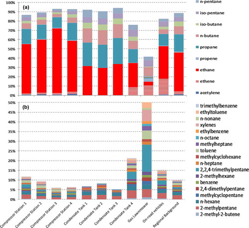
Carbon disulfide is not shown on these figures, since its concentrations were very low—in the range of 0.03–0.05 ppbv. Slightly higher concentrations were recorded in the grab samples collected at the peak of emissions from the Star Shell Road tanks (1.8 and 0.45 ppbv). However, when integrated over an hour, the corresponding concentrations in condensate tank samples 1 and 2 were 0.04 and 0.05 ppbv, respectively.

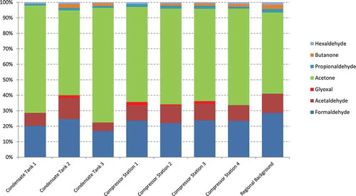
Figure 4 shows the concentrations of carbonyl compounds in the source-oriented samples collected in Phase 1. The full data set is presented in Supplemental Material (Table S6). The composition and concentrations of carbonyls in all samples are very similar to background sample, with acetone, formaldehyde, and acetaldehyde being the most abundant species. No acrolein was detected. This indicates that carbonyl compounds are not present in the emissions from natural gas production facilities and are probably formed mostly from photochemical transformation of gas phase hydrocarbons (Finlayson-Pitts and Pitts, 1999) and/or emitted from variety of combustion sources.

Figure 4. Composition of carbonyl compounds in source samples collected during Phase 1. Percentages shown are volumetric.

Downwind gradient experiment

In the second phase, 7-day time-integrated sampling was conducted at multiple locations downwind of a gas well with condensate tank emissions that were characterized during Phase 1. The measurements at this private residence are intended to serve as a case study of the pollutant gradients at increasing distance downwind of the well tanks relative to the upwind background pollutant concentrations. Figure 2 shows the locations of the sampling sites in relation to the gas well and two condensate tanks.

The concentration of each species was background subtracted using values from the corresponding sample collected at the upwind site (PSSV16). Results are presented in Figure 5a and b, which shows that average levels of VOCs decrease with distance rapidly downwind of the well, approaching background within 70 m for most species. Aromatics (e.g., BTEX) and cycloalkanes are graphed separately from the higher concentration alkanes for clarity (Figure 5a). Benzene concentration at the upwind site was higher than near the residence, possibly due to emissions from trucks or farm vehicles on the adjacent unpaved county road. 1,3-Butadiene was measured but is not included in the charts, since it tended to be near background at all sites. This plot is for the samples beginning May 13, 2010, for which data are valid for all sites.

Figure 5. VOC gradient downwind of a well with condensate tank emissions. (a) Aromatics and cycloalkanes (linear scale); (b) aliphatic hydrocarbons (log scale). Concentrations are background subtracted 7-day averages for the week of May 13, 2010.

The pollutant gradients for hydrocarbons, which had a large variation in concentration between species, can be seen more clearly in Figure 6 by normalizing all of the values to the concentration measured at the site closest to the tanks (PSSV15). The upwind site, PSSV16, is shown at −1600 m distance. All of the alkanes show a similar sharp decrease of 60–80% from site closest to the tanks (˜17 m from the tanks) to the next downwind site (˜67 m from the tanks). Concentrations at the second downwind sites (˜110 m from the tanks) were only slightly lower than from the first downwind site. In contrast to alkanes, the concentration gradients were not as steep and more variable for the BTEX species. This is likely due to the greater local background ambient concentrations of BTEX, especially benzene, as indicated by the higher values obtained for BTEX at PSSV16 relative to alkanes. In addition, 1,3-butadiene does not show an appreciable gradient, as this species is a combustion product not emitted from condensate tanks or gas wells.

Figure 6. The concentration gradient downwind of a well with condensate tank emissions. Values are 7-day averages for the week of May 13, 2010 (week 4), normalized to the concentration nearest the well.

In contrast, the corresponding data for background subtracted carbonyl compounds in Figure 7 show much more uniform concentrations, with the exception of hexaldehyde. Although carbonyl compounds are directly emitted from motor vehicles, a greater portion of these compounds in the ambient air are due to chemical transformation of hydrocarbons in the atmosphere (Finlayson-Pitts and Pitts, 1999).

Figure 7. Aldehyde gradient downwind of a well with condensate tank emissions. Concentrations are background-subtracted averages.

Community saturation monitoring

The second study area was the small community of Shale Creek in Rhome, Texas (see Figure 1). This community is a cluster of approximately 250 occupied houses with a large compressor station located approximately 200 m west-southwest of the community and a high density of gas and oil wells in the surrounding area. The community is located about 20 miles north-northwest of Fort Worth and is entirely single-family homes with no through traffic access. The spatial variations in pollutant concentrations were determined at various distances and directions from the source, sites adjacent to nearby roadways, and a background site located upwind of the community. The study results were placed in context by comparing the measured pollutant concentrations with comparable data from elsewhere in the Barnett Shale area and from urban areas of Dallas-Fort Worth.

Passive and active monitors were located in the backyards of volunteers’ houses throughout the community (sites PSSV01–PSSV07; see Figure 1). Additional passive monitors were located at the southeast corner of the boundary fence (PSSV09) and west entrance to the compressor station (PSSV11), at the perimeter of the community northeast of the plant (PSSV08), next to the adjacent County Line Road (PSSV10), and 1 mile south of Shale Creek community (PSSV12; not shown in Figure 1). We did not have permission to access the compressor station property or the area directly downwind of it, so only monitoring at the fenceline was possible.

A meteorology station was installed at the PSSV01 residential site that recorded hourly wind speed, direction, temperature, and relative humidity for 4 weeks during sampling. Table 3 shows the weekly mean of meteorology parameters from data collected at this site, and Figure S3 (Supplemental Material) displays the frequency of wind direction at this site. As Table 3 and Figure S3 show, the predominant wind direction was from south-southeast. The west or southwest component, which would transport air directly from the compressor station to the community, was relatively minor.

Table 3. Weekly mean of meteorology parameters from data collected at site PSSV01

	Temperature	Relative Humidity	Wind Speed	Easterly Wind Vector	Northerly Wind Vector
Week	(°C)	(%)	(m/sec)	(m/sec)	(m/sec)	RWD
April 22–April 29	18.0	58.7	1.0	−0.09	−0.34	SSE
April 29–May 6	20.1	61.3	1.1	0.00	−0.68	S
May 6–May 13	22.5	62.9	2.0	0.53	−1.31	SSE
May 13–May 20	21.9	77.9	0.7	0.25	−0.09	ESE

Notes: RWD = resultant wind direction. Negative wind vectors indicate prevailing wind from opposite direction.

Volatile organic compounds

VOC concentrations in the Shale Creek community were similar to or lower than at nearby area monitoring stations, especially during week 3 of sampling when the winds were mostly from the southeast and were stronger than during other weeks (see Figure S3). Table S7 shows the 21-day mean concentrations of VOC species quantified from passive Radiello cartridges, listed in the order of increasing distance from the compressor station (see Figure 1). The corresponding data from the TCEQ autoGC sites in Fort Worth and DISH (Texas Commission on Environmental Quality, 2013) averaged over the same time period and long-term Exposure Screening Levels set by TCEQ are also included for reference.

Although the site-to-site differences in concentration of total quantified VOCs is small, some individual species shows larger differences, but not always consistent with the distance from the compressor station. For example, Figure 8 shows the 4-week average concentrations for benzene and n-pentane. Benzene concentrations decrease from the two sites closest to the station (PSSV09 and PSSV11), but increase again at a distant site PSSV07. PSSV10 is close to a road, so it may be influenced by motor vehicle emissions. Benzene concentrations at a residential area located 6 km south of Shale Creek, operated as part of the Fort Worth Natural Gas Air Quality Study during the fall of 2010 (Eastern Research Group, 2011), were very similar (0.197 ± 0.035 ppb) to the mean value for the seven residential sites in Shale Creek (0.213 ppb). Concentrations of n-pentane are more uniform, although also slightly higher at the site along the county road (PSSV10). The background site PSS12, far away from Shale Creek community, had the lowest concentrations for the majority of quantified compounds.

Figure 8. Average (a) benzene and (b) n-pentane concentrations at Shale Creek community sites over 21 days, ordered from left to right according to increased distance from the compressor station. PSSV11: W side of compressor station; PSSV09: SE corner of compressor station, PSSSV08: NE of compressor station; PSSV01–PSSV07: residential sites in Shale Creek community; PSSV10: County Line Road; PSSV12: 1 mile S. Corresponding data from TCEQ autoGC sites are included for comparison.

Concentrations of carbonyl compounds were low and consistent with active sampling performed in Phase 1. Table S8 shows the 21-day average concentrations for measured carbonyls. The most abundant aldehyde in all samples is formaldehyde, followed by acetaldehyde. There is no indication of carbonyl compounds emissions from natural gas production facilities.

Oxides of nitrogen

Figure 9 shows mean (averaged over 3-week monitoring period) NO and NO₂ concentrations for passive samples collected at Shale Creek Community (SO₂ concentrations were very low, at or below the detection limit of the method, so they are not shown). Concentrations are higher at sites nearest the compressor station and at site PSSV10 located next to County Line Road. The background site PSSV12 had the lowest NO values. NO₂ concentrations at the residential sites were similar to those at the Fort Worth State and Local Air Monitoring Station (SLAMS) site (data obtained from EPA Air Quality System Web site), but NO was somewhat higher.

Figure 9. Mean NO and NO₂ concentrations over sampling period. PSSV11: W side of compressor station; PSSV09: SE corner of compressor station, PSSV08: NE of compressor station; PSSV01–PSSV07: residential sites in Shale Creek community; PSSV10: County Line Road; PSSV12: 1 mile S. Sites are ordered according to increased distance from the compressor station. Corresponding data from a monitoring station in Fort Worth are also shown for comparison.

Particulate matter

PM_2.5 filter samples were collected in parallel with passive samples at six residential locations in the Shale Creek community where electrical power for the samplers was available. Teflon filters were analyzed for PM_2.5 mass and elements Na to U, and quartz filters were analyzed for OC, EC, and PAHs. Figure 10 shows the concentrations of PM_2.5 mass and the fractions of OC and EC for each week of sampling. Both Teflon and quartz filters from the first week of monitoring at the PSSV02 site were lost due to sampler malfunctions and another Teflon filter sample from this site (April 29–May 6) was invalidated due to insect contamination. At site PSSV03, both filters from week 2 were lost due to a power outage and quartz filters from weeks 1 and 3 were invalidated due to filter clogging.

Figure 10. Composition of PM_2.5 mass for all 4 weeks of sampling at Shale Creek sites. Error bars indicate the uncertainty of the gravimetric mass measurement.

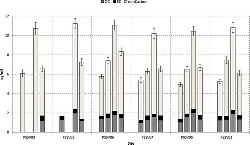
There is little variation among sites, suggesting that the fine PM concentrations are dominated by regional rather than local sources. Note that OC indicates the mass of carbon contained in organic species, not the total organic species mass (OM). Assuming an OM/OC ratio of 2:1 (El-Zanan et al., 2005, 2009; Lowenthal et al., 2009), OM contributes in the range of 30–50% to PM_2.5 mass. EC concentrations were below 0.5 μg/m³, contributing 4–8% to PM_2.5 mass. The ratio of EC to total carbon, which is a useful indicator of the relative importance of diesel engine exhaust, ranged from 15% to 30% which is similar to that observed in urban areas (Tetra Tech, Inc., 2013). In contrast to the VOC species, which tended to be lower during the third week of sampling, PM_2.5 and OC concentrations were the highest in week 3 at all monitoring sites when the predominant wind was from the southeasterly direction (see Figure 10). This may indicate transport from the Dallas-Fort Worth metropolitan area. The Teflon filters were also analyzed for elements by X-ray fluorescence to determine the main components of PM_2.5 besides OC and EC. About 40% of the noncarbonaceous mass was ammonium sulfate, with most of the remainder accounted for by elements commonly found in resuspended soil (after adjusting to account for common oxide forms).

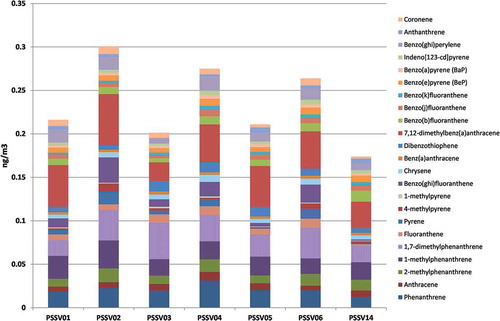
The quartz filters were also analyzed for 45 particle-associated PAHs using a GC/MS method. Table S9 (Supplemental Material) lists PAHs quantified for this study and their concentrations, and Figure 11 shows the averaged over 4 weeks concentrations of the most abundant PAHs. The concentrations of PAHs in all samples were low, in the range of picograms/m³. The most abundant PAHs in most of the samples included 1,7-dimethylphenanthrene, 7,12-dimethylbenz[a]anthracene, methylphenanthrene isomers, phenanthrene, benzo[g,h,i]fluoranthene, and chrysene. These PAHs and methylated PAHs are found in diesel engine exhaust (Zielinska et al., 2004a, 2004b), which is most likely their source in this study.

Figure 11. Average PAH concentrations at Shale Creek community sites (PSSV01–PSSV06) and Star Shell Road site (PSSV14).

VOC source apportionment

The measured VOCs were apportioned to sources using the CMB receptor model. Good model performance was achieved for 90% of the ambient sample data from the Shale Creek area using the default set of source profiles and fitting species, and the relative contributions attributed to the source categories were similar for all sites within the community, giving a high degree of credibility to the model results. Performance was not as good for the Star Shell Road sites (PSSV15 and PSSV16), and satisfactory results could not be obtained for any of the samples from site 14, possibly due to local emissions from an unrepresented source. However, those sites were only included as a demonstration of model sensitivity. Of the default profiles listed in Table 2, only four were repeatedly utilized by the CMB program to create the best solution: Tank_Vent, NG, HDD, and LDGV. The LAWNMWR profile was only used for a few samples and was combined in the results with the LDGV profile under Gasoline Engines. As noted earlier, the profiles derived from samples collected at the fenceline of gas processing plants did not turn out to be sufficiently distinct from the regional background.

Figure 12a, b, and c and Table S10 (Supplemental Material) show the results of source apportionment for the sum of all measured hydrocarbons (a), benzene (b), and n-pentane (c). For the sum of all measured hydrocarbons, the dominant source category at the Shale Creek residential sites was diesel truck emissions to which 40–50% of total NMHCs was attributed. Condensate tank emissions were estimated to contribute the next largest fraction: 24 ± 4%. The compressed natural gas (CNG) profile was linked to 10–20% of NMHCs, but it is possible that this may include some misapportionment, since the profile is similar to the lower-molecular-weight components of aged automobile exhaust. Gasoline engines, including lawnmowers, accounted for the remaining 10–20% of the total. Apportionments for the sites nearest the gas processing plant or the highway indicated slightly higher CNG and condensate tank influence. As expected, the apportionments for the sites at Star Shell Road were much more strongly dominated by condensate tank emissions (70–98%), with very little motor vehicle contribution.

Figure 12. Mean relative source contribution estimates of four source categories to (a) total hydrocarbons, (b) benzene, and (c) pentane for each monitoring site.

Examining the apportionments for individual organic compounds, the model predicted that more than 70% of pentane was attributed to fugitive emissions of natural gas, whereas more than 80% of benzene was due to engine emissions. Xylenes were almost entirely attributed to motor vehicle emissions at most sites, except at the Star Shell Road site, which is far from any public roads. In summary, CMB results indicate that motor vehicle exhaust is the dominant source of VOCs in the Shale Creek community, but emissions from natural gas extraction make a substantial contribution to some hydrocarbons <C7 (see Figure 12); however, none of them reach a level for health concerns (see Table S7).

Summary and Conclusion

The purpose of this study was to provide a better understanding of the potential contributions of emissions from gas production operations to population exposure to air toxics in the Barnett Shale region. This goal was approached using a combination of chemical characterization of the VOC emissions from active wells, saturation monitoring for gaseous and particulate pollutants in a residential community located near active gas/oil extraction and processing facilities, source apportionment of VOCs measured in the community using the CMB receptor model, and direct measurements of the pollutant gradient downwind of a gas well with high VOC emissions.

Due to access restrictions, we were not able to obtain specific source composition profiles for compressor stations or well drilling operations, but several samples from well-head condensate tank venting emissions were collected and used to create a source profile of this major source of VOC emissions in the study area. The main characteristics of the condensate tank venting emissions were the following:

• The most abundant nonmethane VOC species emitted from the condensate tank adjacent to gas wells were ethane, propane, n-butane, isobutane, isopentane, and n-pentane. These species account for over 90% of VOC emissions.

• The remaining ˜10% included mostly of 2- and 3-methylpentane, n-hexane, methylcyclopentane, cyclohexane, 2-methylhexane, 1-heptene, methylcyclohexane, n-heptane, and n-octane.

• Aromatic hydrocarbons, such as benzene, toluene, and xylenes, were much less abundant and accounted for approximately 0.1–0.2% of nonmethane VOC emissions.

• Carbonyl compounds were not emitted from the condensate tanks located next to the gas wells.

Saturation monitoring over 3–4 weeks at a residential community adjacent to a gas processing facility gave the following results:

• The average concentrations of VOC species measured by passive samplers were low, generally below 1 ppb. These concentrations are comparable or slightly higher than those measured by TCEQ over the same time period with continuous autoGCs in Fort Worth and DISH, and much lower than those specified by the short- and long-term health-based Air Monitoring Comparison Values (e.g., 180 and 1.4 ppbv, respectively, for benzene).

• PM_2.5 concentrations during the study were below the National Ambient Air Quality Standard (NAAQS) and spatially uniform. The aerosol comprised 30–50% organic compounds, with ammonium sulfate and soil making up most of the balance.

The generally low concentrations measured were consistent with the gradient measurements made downwind of a condensate tank with significant venting activity where a steep exponential decrease in emission concentrations was observed from the site closest to an emission source to the next downwind site located ˜67 m from the tank. The concentrations of emissions from the tank decreased to near background levels at a distance of ˜100 m. This steep decrease in concentration is very similar to that observed in other studies (Fujita et al., 2014; Zhu et al., 2002), where measured downwind pollutant concentrations decreased to upwind background levels within about 100 m of a roadway.

Applying the saturation monitoring VOC data and source profiles representing gas and condensate fugitive emissions and diesel and gasoline engine exhaust, the Chemical Mass Balance receptor model yielded the following results:

• The dominant source category of total NMHCs was motor vehicle emissions, to which 64 ± 10% was attributed for the residential site locations. Combined natural gas and condensate tank emissions were estimated to contribute 36 ± 10% at the residential sites, and up to 48% at the sites nearer the compressor station.

• For individual organic compounds, the CMB receptor model predicted that more than 70% of pentane is due to condensate tank emissions, whereas more than 80% of benzene is attributed to vehicle exhaust, primarily diesel.

Overall, the study results indicate that air quality impacts due to individual gas wells and compressor stations are not likely to be discernible beyond a distance of approximately 100 m in the downwind direction. However, source apportionment results indicate a significant contribution to regional VOCs from gas production sources, particularly for lower-molecular-weight alkanes (<C6). In addition, the existence of similar mean concentrations of benzene and other mobile source air toxics and urban-level EC/TC ratios in an area with little residential or commercial development may be indicative of the impact of increased heavy-duty diesel on- and off-road vehicles related to gas production.

Regarding the general applicability of these conclusions, several caveats should be considered:

• Due to contractual constraints, the study was performed in April–May when the temperatures were not high and winds were mostly from southeasterly direction. Results might differ if the study had been performed at a different time of year. Data from the TCEQ’s Northwest Fort Worth monitoring station (Texas Air Monitoring Information System Web Interface) indicate that, for the years 2008–2012, the mean concentrations of lighter hydrocarbons associated with gas production are similar in spring and summer but approximately 70% higher in fall and winter. Motor vehicle exhaust–related compounds show a weaker seasonal trend (50% higher in fall and winter).

• The compressor station adjacent to the Shale Creek community was typically downwind of the community, and observed gradients in pollutant concentrations were small and cannot be unambiguously associated with proximity to the compressor station. Slightly higher concentrations were observed at a few sites closer to roads.

• Approximately two dozen well sites were surveyed in Wise County in the areas surrounding Rhome, Decatur, Aurora, Boyd, New Fairview, Alvord, Bridgeport, Runaway Bay, Chico, Paradise, and Allison. This survey was certainly not complete, taking into account the thousands of well sites and compressor stations active in the Barnett Shale area. Thus, this study should be regarded as a pilot study and not a comprehensive mapping of emissions from all sources in the area.

• We were denied access to most active well sites and compressor stations in the area. This limited our ability to collect representative source profiles for all gas and oil extraction and processing activity in the area. The addition of profiles for well drilling, hydraulic fracturing, and gas processing might increase the apportionments for petroleum extraction–related sources.

• The conclusions drawn from this study should be considered tentative and should be supported by a larger study or data from other studies covering all seasons that provides statistical confirmation of the study results. In addition to data for other seasons, spatial pollutant gradients should be obtained for other communities in the region.

Acknowledgment

The authors acknowledge Mark McDaniel and Anna Cunningham of DRI for their assistance in sample analyses and Dr. Eric Fujita for helpful discussions.

Supplemental Material

Supplemental data for this article can be accessed at http://dx.doi.org/10.1080/10962247.2014.954735.

Funding

This project was funded by the Mickey Leland National Urban Air Toxics Research Center. The authors thank American Petroleum Institute for providing funds to write this paper.

Additional information

Notes on contributors

Barbara Zielinska

Barbara Zielinska is research professor, Vera Samburova is assistant research professor, and Dave Campbell is associate research scientist at Desert Research Institute.

Dave Campbell

Barbara Zielinska is research professor, Vera Samburova is assistant research professor, and Dave Campbell is associate research scientist at Desert Research Institute.

Vera Samburova

Barbara Zielinska is research professor, Vera Samburova is assistant research professor, and Dave Campbell is associate research scientist at Desert Research Institute.

References

- Armendariz, A. 2009. Emissions from Natural Gas Production in the Bernett Shale Area And Opportunities for Cost-Effective Improvements. Final report prepared for the Environmental Defense Fund, Washington, DC.
- Branosky, E., A. Stevens, and S. Forbes. 2012. Defining the Shale Gas Life Cycle: A Framework for Identifying and Mitigating Environmental Impacts. Washington, DC: World Resources Institute.
- Bunch, A.G., C.S. Perry, L. Abraham, D.S. Wikoff, J.A. Tachovsky, J.G. Hixon, J.D. Urban, M.A. Harris, and L.C. Haws. 2014. Evaluation of impact of shale gas operations in the Barnett Shale region on volatile organic compounds in air and potential human health risks. Sci. Total Environ. 468:832–842. doi:10.1016/j.scitotenv.2013.08.080
- Chow, J.C., J.G. Watson, L.C. Pritchett, W.R. Pierson, C.A. Frazier, and R.G. Purcell. 1993. The DRI thermal optical reluctance carbon analysis system—Description, evaluation and applications in United States air-quality studies. Atmos. Environ. 28:1185–1201.
- Eastern Research Group. 2011. City of Fort Worth Natural Gas Air Quality Study, Final Report. Prepared for City of Fort Worth, Fort Worth, TX. http://fortworthtexas.gov/uploadedFiles/Gas_Wells/AirQualityStudy_final.pdf (accessed July 2011).
- El-Zanan, H.S., D.H. Lowenthal, B. Zielinska, J.C. Chow, and N. Kumar. 2005. Determination of the organic aerosol mass to organic carbon ratio in IMPROVE samples. Chemosphere 60:485–496. doi:10.1016/j.chemosphere.2005.01.005
- El-Zanan, H.S., B. Zielinska, L.R. Mazzoleni, and D.A. Hansen. 2009. Analytical determination of the aerosol organic mass-to-organic carbon ratio. J. Air Waste Manage. Assoc. 59:58–69. doi:10.3155/1047-3289.59.1.58
- Finlayson-Pitts, B.J., and J.N. Pitts. 1999. Chemistry of the Upper and Lower Atmosphere: Theory, Experiments, and Applications. London, UK: Elsevier Science.
- Fujita, E.M., D.E. Campbell, W.P. Arnott, T. Johnson, and W. Ollison. 2014. Concentrations of mobile source air pollutants in urban microenvironments. J. Air Waste Manage. Assoc. 64:743–758. doi:10.1080/10962247.2013.872708
- Fujita, E.M., D.E. Campbell, B. Zielinska, W.P. Arnott, and J.C. Chow. 2011. Concentrations of Air Toxics in Motor Vehicle-Dominated Environments. Final report to Health Effects Institute, Boston, MA. http://pubs.healtheffects.org/view.php?id=354 (accessed December 2013).
- Fujita, E.M., D.E. Campbell, B. Zielinska, J.C. Chow, C.E. Lindhjem, A. DenBleyker, G.A. Bishop, B.G. Schuchmann, D.H. Stedman, and D.R. Lawson. 2012. Comparison of the MOVES2010a, MOBILE6.2, and EMFAC2007 mobile source emission models with on-road traffic tunnel and remote sensing measurements. J. Air Waste Manage. Assoc. 62: 1134–1149. doi:10.1080/10962247.2012.699016
- Fujita, E.M., R.E. Keislar, J.L. Bowen, W. Goliff, F. Zhang, L.H. Sheetz, M.D. Keith, J.C. Sagebiel, and B. Zielinska. 1999. 1998 Central Texas On-Road Hydrocarbon Study. Final report prepared for the Texas Department of Transportation, Austin, TX.
- Fujita, E.M., B. Mason, D.E. Campbell, and B. Zielinska. 2009. Harbor Community Monitoring Study—Saturation Monitoring. Final report to California Air Resources Board, Sacramento, CA. http://www.arb.ca.gov/research/apr/past/05-304.pdf (accessed January 2014).
- Hendler, A., J. Nunn, and J. Lundeen. 2009. VOC Emissions from Oil and Condensate Storage Tanks. Texas Environmental Research Consortium. http://files.harc.edu/Projects/AirQuality/Projects/H051C/H051CFinalReport.pdf (accessed December 2013).
- Jackson, R.B., A. Vengosh, T.H. Darrah, N.R. Warner, A. Down, R.J. Poreda, S.G. Osborn, K. Zhao, and J.D. Karr. 2013. Increased stray gas abundance in a subset of drinking water wells near Marcellus shale gas extraction. Proc. Natl. Acad. Sci. U. S. A. 110:11250–11255. doi:10.1073/pnas.1221635110
- Krzyzanowski, J. 2012. Environmental pathways of potential impacts to human health from oil and gas development in northeast British Columbia, Canada. Environ. Rev. 20:122–134. doi:10.1139/a2012-005
- Lev-On, M., C. LeTavec, J. Uihlein, K. Kimura, T.L. Alleman, D.R. Lawson, K. Vertin, M. Gautam, G.J. Thompson, W.S. Wayne, N. Clark, R. Okamoto, P. Rieger, G. Yee, B. Zielinska, J. Sagebiel, S. Chatterjee, and K. Hallstrom. 2002. Speciation of Organic Compounds from the Exhaust of Trucks and Buses: Effect of Fuel and After-Treatment on Vehicle Emission Profiles. Society of Automotive Engineers, I., Paper No. 2002-01-2873. Paper from the Society of Automotive Engineers (SAE) Powertrain and Fluid Systems Conference and Exhibition, October 2002, San Diego, California. Warrendale, PA: Society of Automotive Engineers, Inc.
- Lowenthal, D., B. Zielinska, B. Mason, S. Samy, V. Samburova, D. Collins, C. Spencer, N. Taylor, J. Allen, and N. Kumar. 2009. Aerosol characterization studies at Great Smoky Mountains National Park, summer 2006. J. Geophys. Res. Atmos. 114: D08206. doi:10.1029/2008JD011274
- Mason, J.B., E.M. Fujita, D.E. Campbell, and B. Zielinska. 2011. Evaluation of passive samplers for assessment of community exposure to toxic air contaminants and related pollutants. Environ. Sci. Technol. 45:2243–2249. doi:10.1021/es102500v
- McKenzie, L.M., R. Guo, R.Z. Witter, D.A. Savitz, L.S. Newman, and J.L. Adgate. 2014. Birth outcomes and maternal residential proximity to natural gas development in rural Colorado. Environ. Health Perspect. 122:412–417. doi:10.1289/ehp.1306722
- McKenzie, L.M., R.Z. Witter, L.S. Newman, and J.L. Adgate. 2012. Human health risk assessment of air emissions from development of unconventional natural gas resources. Sci. Total Environ. 424:79–87. doi:10.1016/j.scitotenv.2012.02.018
- Moore, C.W., B. Zielinska, G. Petron, and R.B. Jackson. 2014. Air impacts of increased natural gas acquisition, processing, and use: A critical review. Environ. Sci. Technol. 48:8349–8359. doi:10.1021/es4053472
- Tejada, S.B. 1986. Evaluation of silica-gel cartridges coated insitu with acidified 2,4-dinitrophenylhydrazine for sampling aldehydes and ketones in air. Int. J. Environ. Anal. Chem. 26:167–185. doi:10.1080/03067318608077112
- Tetra Tech, Inc. 2013. Phase III of the LAX Air Quality and Source Apportionment Study—Final Report. http://www.lawa.org/airQualityStudy.aspx?id=7716 (accessed December 2013).
- Texas Railroad Commission. 2010. Production data query system. http://webapps.rrc.state.tx.us/PDQ/generalReportAction.do (accessed November 2013).
- Texas Railroad Commission. 2013. Barnett Shale for RRC—Content page. http://www.rrc.state.tx.us/barnettshale (accessed November 2013).
- U.S. Energy Information Administration, 2013. Natural gas statistics and analysis. http://www.eia.gov/naturalgas/ (accessed December 2013).
- U.S. Environmental Protection Agency. 1999a. Method TO-11A. Determination of Formaldehyde in Ambient Air Using Adsorbent Cartridge Followed by High Performance Liquid Chromatography (HPLC) in Compendium of Methods for the Determination of Toxic Organic Compounds in Ambient Air, 2nd ed. Cincinnati, OH: Center for Environmental Research Information, Office of Research and Development, U.S. Environmental Protection Agency.
- U.S. Environmental Protection Agency. 1999b. Method TO-15. Determination of Volatile Organic Compounds (VOCs) in Air Collected in Specially-Prepared Canisters and Analyzed by Gas Chromatography/Mass Spectrometry (GC/MS), 2nd ed. EPA/625/R-96/010b. Cincinnati, OH: Center for Environmental Research Information, Office of Research and Development, U.S. Environmental Protection Agency.
- Warner, N.R., R.B. Jackson, T.H. Darrah, S.G. Osborn, A. Down, K. Zhao, A. White, and A. Vengosh. 2012. Geochemical evidence for possible natural migration of Marcellus Formation brine to shallow aquifers in Pennsylvania. Proc. Natl. Acad. Sci. U. S. A. 109:11961–11966. doi:10.1073/pnas.1121181109
- Watson, J.G., J.C. Chow, and C.A. Frazier. 1999. X-ray fluorescence analysis of ambient air samples. In Elemental Analysis of Airborne Particles, ed. S. Landsberger and M. Creatchman, 67–96. Amsterdam, the Netherlands: Gordon and Breach Science.
- Watson, J.G., N.F. Robinson, C.W. Lewis, C.T. Coulter, J.C. Chow, E.M. Fujita, D.H. Lowenthal, T.L. Conner, R.C. Henry, and R.D. Willis 1997. Chemical Mass Balance (CMB) Model version 8 user’s manual. Prepared for U.S. Environmental Protection Agency, Research Triangle Park, NC, by Desert Research Institute, Reno, NV. http://www.epa.gov/scram001/receptor_cmb.htm (accessed January 2014).
- Zhu, Y.F., W.C. Hinds, S. Kim, S. Shen, and C. Sioutas. 2002. Study of ultrafine particles near a major highway with heavy-duty diesel traffic. Atmos. Environ. 36:4323–4335. doi:10.1016/S1352-2310(02)00354-0
- Zielinska, B., E. Fujita, and D. Campbell 2011. Monitoring of Emissions from Barnett Shale Natural Gas Production Facilities for Population Exposure Assessment. Final Report No. 19 to Mickey Leland National Urban Air Toxic Research Center, Houston, TX. https://sph.uth.edu/mleland/attachments/DRI-Barnett%20Report%2019%20Final.pdf (accessed November 2013).
- Zielinska, B., J. Sagebiel, W.P. Arnott, C.F. Rogers, K.E. Kelly, D.A. Wagner, J.S. Lighty, A.F. Sarofim, and G. Palmer. 2004a. Phase and size distribution of polycyclic aromatic hydrocarbons in diesel and gasoline vehicle emissions. Environ. Sci. Technol. 38:2557–2567. doi:10.1021/es030518d
- Zielinska, B., J. Sagebiel, J.D. McDonald, K. Whitney, and D.R. Lawson. 2004b. Emission rates and comparative chemical composition from selected in-use diesel and gasoline-fueled vehicles. J. Air Waste Manage. Assoc. 54:1138–1150. doi:10.1080/10473289.2004.10470973