Emissions Variability Processor (EMVAP): Design, evaluation, and application

Abstract

Emissions of pollutants such as SO₂ and NOx from external combustion sources can vary widely depending on fuel sulfur content, load, and transient conditions such as startup, shutdown, and maintenance/malfunction. While monitoring will automatically reflect variability from both emissions and meteorological influences, dispersion modeling has been typically conducted with a single constant peak emission rate. To respond to the need to account for emissions variability in addressing probabilistic 1-hr ambient air quality standards for SO₂ and NO₂, we have developed a statistical technique, the Emissions Variability Processor (EMVAP), which can account for emissions variability in dispersion modeling through Monte Carlo sampling from a specified frequency distribution of emission rates. Based upon initial AERMOD modeling of from 1 to 5 years of actual meteorological conditions, EMVAP is used as a postprocessor to AERMOD to simulate hundreds or even thousands of years of concentration predictions. This procedure uses emissions varied hourly with a Monte Carlo sampling process that is based upon the user-specified emissions distribution, from which a probabilistic estimate can be obtained of the controlling concentration. EMVAP can also accommodate an advanced Tier 2 NO₂ modeling technique that uses a varying ambient ratio method approach to determine the fraction of total oxides of nitrogen that are in the form of nitrogen dioxide. For the case of the 1-hr National Ambient Air Quality Standards (NAAQS, established for SO₂ and NO₂), a “critical value” can be defined as the highest hourly emission rate that would be simulated to satisfy the standard using air dispersion models assuming constant emissions throughout the simulation. The critical value can be used as the starting point for a procedure like EMVAP that evaluates the impact of emissions variability and uses this information to determine an appropriate value to use for a longer term (e.g., 30-day) average emission rate that would still provide protection for the NAAQS under consideration. This paper reports on the design of EMVAP and its evaluation on several field databases that demonstrate that EMVAP produces a suitably modest overestimation of design concentrations. We also provide an example of an EMVAP application that involves a case in which a new emission limitation needs to be considered for a hypothetical emission unit that has infrequent higher-than-normal SO₂ emissions.

Implications

Emissions of pollutants from combustion sources can vary widely depending on fuel sulfur content, load, and transient conditions such as startup and shutdown. While monitoring will automatically reflect this variability on measured concentrations, dispersion modeling is typically conducted with a single peak emission rate assumed to occur continuously. To realistically account for emissions variability in addressing probabilistic 1-hr ambient air quality standards for SO₂ and NO₂, the authors have developed a statistical technique, the Emissions Variability Processor (EMVAP), which can account for emissions variability in dispersion modeling through Monte Carlo sampling from a specified frequency distribution of emission rates.

Introduction

Emissions of pollutants such as SO₂ and NOx can vary substantially from normal or steady-state conditions during startup, shutdown, malfunction, or stack-bypass conditions. During these transient periods, peak emissions can be much higher than the emissions for typical operations.

The Electric Power Research Institute (EPRI, 2014) has developed and released to the public an advanced technique, the Emissions Variability Processor (EMVAP), which can account for emissions variability for a variety of purposes. EMVAP is designed to use an emission probability distribution to better approximate the ideal modeling case that uses actual hourly emissions, while maintaining some level of conservatism. While the use of actual emissions simulates concentrations that could have been measured at numerous “virtual monitors,” we note that modeling of future operations must employ an estimate of future emissions in the form of a distribution function. EMVAP provides a procedure for using finite years of actual meteorological conditions modeled with unit emissions combined with hourly emissions drawn randomly from the user-specified distribution to create many simulated years of concentration predictions.

This paper describes the design of the EMVAP system as well as testing of EMVAP against modeling results with actual hourly emissions for several electric generating units (EGUs), some of which were used in the original AERMOD evaluation by the U.S. Environmental Protection Agency (EPA) of the AERMOD model (Cimorelli et al., 2005; Perry et al., 2005). The authors understand that for providing assurance to reviewing environmental agencies, it is important that EMVAP should provide predictions of design concentrations with the emissions distributions as created according to EMVAP user instructions that are at least as high as predicted design concentrations using actual hourly emissions. In addition, we provide an example application of EMVAP to demonstrate that the modeling of an emission distribution can show how a long-term average emission rate comprised of a mixture of typical as well as transient peak emissions can be protective of a probabilistic 1-hr NAAQS (for SO₂ and NO₂).

Review of EMVAP Design and Operation

Evaluation of emissions distribution

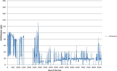
Consider the hourly frequency distribution of SO₂ emissions from the source shown in Figure 1. As shown in the figure, the emissions from this source vary greatly on an hour-to-hour basis. While the majority of the hours have emissions in the 20 g/sec range, the peak emissions that occur only rarely are approximately 130 g/sec, or 6.5 times higher than the typical emissions. Since permit limits usually have a margin to allow for operational flexibility, the permit limit for this source might be set to 200 g/sec. Typical compliance modeling procedures as described in Section 8 of the EPA modeling guidance (Appendix W: EPA, 2005) would specify that 200 g/sec would need to be modeled as if this occurs continuously, even though that emission rate is an order of magnitude higher than the typical emissions of the facility. Clearly, this would result in highly exaggerated modeled impacts relative to actual impacts that can be estimated by modeling the actual hourly emissions.

Figure 1. Example time series of variable SO₂ emissions from a single source.

In recognition of this issue, the EPA (2014a) issued new draft guidance in the form of “Technical Assistance Documents” (TADs) for modeling associated with implementation of the SO₂ NAAQS in May 2013 and again in January 2014 with updates. The modeling TAD indicates that modeling assessments for the purpose of demonstrating NAAQS compliance from existing sources should use actual hourly emissions as model input, in addition to actual stack heights.

While this approach would work for assessing NAAQS compliance for existing sources, it is more challenging to accommodate varying emissions for sources yet to operate, or for existing sources subject to modification. While AERMOD has the capability of modeling emission changes that can be scheduled, it has no capability for modeling emission variations of an unpredictable nature, such as those due to fuel sulfur variability, as well as transient conditions such as startup, shutdown, and maintenance.

While the modeling of the future operation of a variable emissions source cannot use actual historical emissions, it can, in principal, make use of an emissions distribution, perhaps based on historical emissions, and assign, on a probabilistic basis, predicted concentrations for hundreds or thousands of simulated years of operation. In essence, this is how EMVAP operates. The distribution of representative actual past emissions from existing sources can help to guide the selection of the emissions distribution by defining discrete cases, or emission “bins,” each with a probability of occurrence and an assigned emission rate. EMVAP can accommodate more than one source with variable emissions, each with its own set of emission bins. However, some sources have relatively constant emissions, and an hourly sequence of background concentrations is also a component of the total concentration; EMVAP is designed to accommodate multiple sets of both variable and constant source concentration files generated by AERMOD.

The analysis of emissions variability from existing units is an essential part of the EMVAP modeling system. For sources that have a suitably long-term electronic record of hourly emissions (at least 1 year in duration) and, if available, corresponding stack temperature and velocity hourly data, the Emissions Distribution (EMDIST) preprocessor, a component of the EMVAP modeling system, can be used as a tool to help guide and inform the selection of an appropriate EMVAP emissions distribution. EMDIST sorts hourly emissions and stack parameter data from a source into emission bins according to user instructions that can be used for input into the EMVAP program.

Each emission bin used in EMVAP is defined by a probability, emission rate, and stack parameters (exit velocity and temperature). These bins, taken together, define the user’s characterization of the emissions distribution (and associated exhaust parameters or even separate stacks in the case of a bypass operation) for various bins to be modeled.

An example of an EMDIST analysis, as applied to the example emission time series in Figure 1, is available by constructing a cumulative emissions distribution and then assigning emission bins that “cover” the cumulative emission distribution, as shown in the bin rectangles in Figure 2.

Figure 2. Emission bins from time series of variable SO₂ emissions from a single source.

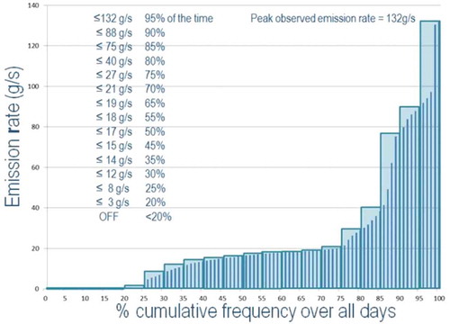
The design of the bin widths and their number is at the discretion of the EMVAP user (frequencies as low as 0.1% are allowed in EMVAP), but they are shown in this example as 20 bins, each of equal (5%) frequency. Note that the space under the rectangles indicates that the overall average emission rate assumed by EMVAP in this case would be higher than the actual emissions used to create the emission bins. This is one aspect of EMVAP design that provides some degree of conservatism.

The list of emission bins and their probabilities shown in Figure 2 are an example of input to the EMVAP emissions distribution processor. The figure shows that the peak emissions of approximately 132 g/sec at this facility occur less than 5% of the time, while the actual emissions are less than one-third of that value nearly 85% of the time.

Monte Carlo sampling with EMVAP processing

The EMVAP system is a postprocessor for dispersion models such as AERMOD that computes hourly concentrations. EMVAP use is not limited to only AERMOD, since it can use hourly concentration output from any model as long as the output is provided in AERMOD output format. As noted earlier, the standard practice of using constant emissions in dispersion models does not properly account for the inherent variability in emission rates, which is important in realistically determining compliance with the probabilistic short-term (1-hr) National Ambient Air Quality Standards (NAAQS) for NO₂ and SO₂ promulgated in 2010. EMVAP is designed to realistically model variable emission sources with respect to probabilistic short-term NAAQS by incorporating a frequency distribution of emission rates for the modeled sources, as shown in the example provided in Figures 1 and 2. Using a Monte Carlo approach, EMVAP can generate a statistical analysis based on thousands of annual simulations and thereby provide robust modeling results for use in compliance demonstrations.

After the emission bins are determined, the next step in the EMVAP process is to run AERMOD with up to 5 actual years of meteorological data for each emission bin and each source. These runs use a constant emission rate of 1 g/sec and the appropriate stack parameters for the source being evaluated with EMVAP. It is possible to use EMVAP for more than one variable source as well as a set of constant emission sources (as well as background), which can be added together in the final processing. Once the AERMOD runs with unit emissions are made for each source and emission bin, the EMVAP run can be made that reads these unit emission file results.

EMVAP uses a preselected series of 500,000 randomly generated integers (from 1 to 1000; from which EMVAP can use different starting points, or “seeds” for different sources, if appropriate) to determine how to assemble the simulated hour-by-hour model concentrations. These concentrations are scaled from the AERMOD predictions from unit emissions over all receptors that were generated from the 1 to 5 years of actual meteorological conditions prior to the use of the EMVAP postprocessor, run for each source with variable emissions. For each hour created in the simulated concentration output file for each variable source, EMVAP selects a random integer (already preselected, as just noted) between 1 and 1000. This value is used to determine what emission bin is selected for that hour from the emissions distribution. For example, for the 20 emission bins shown in Figure 2, a random number of 974 would indicate that the 20th emission bin with an emission rate of 132 g/sec is selected. For that hour and source, the concentrations available from the model runs with the 20th bin source would be extracted from the output file already available, multiplied by 132, and then written to a new concentration file being created for that simulated year.

Note that the concentrations being created for each simulated year are written to a temporary file. Once the full year of the simulated concentrations is created, EMVAP will then determine the concentration statistic (EPA calls this the “design concentration”) that is relevant to the particular pollutant (99th or 98th percentile day for SO₂ or NO₂, respectively). Once all of the simulated years are produced and the statistics are stored, the final step is to rank and output the statistics for the distribution of design concentrations over all simulated years.

While EMVAP includes the capability to randomly sample hourly emission rates according to a user-specified distribution, EMVAP does not address other variations, such as meteorological conditions, that would occur over a long period that equals or exceeds the entire operational period of an emissions source. The degree to which meteorological variability affects modeled concentrations is addressed in EPA Appendix W guidance (EPA, 2005), which specifies that the use of at least 1 year of on-site meteorological data or 5 years of off-site meteorological data is sufficient to provide a sufficiently robust estimate to assess compliance with ambient standards. Thus, the basic modeled concentrations (normalized to unit emissions) are produced using 1 to 5 years of actual meteorology. For each synthetic year (or “realization”) of concentrations produced from this basic set of information, a random number is selected on an hourly basis with a probability of being linked to an emission rate that is defined by the EMVAP user. It is important to keep in mind that the sequence of hours is associated with different meteorological conditions. Since this selection of emissions is randomized hour by hour, each synthetic year of concentrations produced is a different sequence of emission rates that is linked to the sequence of varying meteorological conditions. Since the likelihood of high predicted concentrations is a factor of both meteorological conditions and emission rates, the fact that the emission rates change for each synthetic year in a different sequence produces a potentially significant variation of results from synthetic year to synthetic year.

Although actual series of emissions show autocorrelations (i.e., high emission hours often occur in clusters), a conservative feature of EMVAP serves to randomly distribute the high emission hours evenly (on average) throughout each simulated year. The conservatism of the EMVAP technique is associated with the form of the EPA’s 1-hr standards for SO₂ and NO₂. These standards select the highest hourly concentration in each day and thus disregard the concentrations for all of the other hours that may cluster around the hour with the maximum concentration. The daily maximum 1-hr concentration is then evaluated with a statistical form of the standard.

For example, the SO₂ NAAQS is the 99th percentile among all daily peak hourly concentrations. The way the hourly concentrations are processed for comparison to the standard is that only the highest hour’s concentration for each day is evaluated. This results in 365 or 366 values for each receptor per year, of which the fourth highest is saved. In actual practice, high emission hours tend to be clustered in a sequence of emissions during a given day. However, emissions that cause high hourly concentrations that are clustered in the same day only count as one day out of 365 (or 366), leaving three more days that need to have high concentrations at the same receptor in order to be counted in the context of the standard. The way that EMVAP randomizes hourly emissions does not account for clustering, such that higher emissions are spread over a greater number of days per year than would be expected if hourly emissions were autocorrelated. Such clustering would significantly complicate EMVAP and would add more accounting burdens on sources that exhibit emissions clustering. EMVAP tends to more randomly disperse those high emission hours over more days (unclustered), and since only one hour of a high concentration counts for that day, the same number of high emission hours will have a greater chance of being populated over more days in EMVAP than in real-world practice due to the lack of intentional clustering in EMVAP. This will lead to having more days with at least one hour of high concentrations, and thus the fourth highest day (for SO₂) will more likely have a higher concentration with EMVAP.

Use of Advanced Ambient Ratio Method Tier 2 (Arm2) NO₂ Capability in EMVAP

Oxides of nitrogen (NOx) gases are emitted by combustion processes mostly in the form of NO (nitric oxide), and in the form of NO₂ (nitrogen dioxide) for a small percentage of the emissions. Within several kilometers of an emission source, the primary mechanism for transforming NO to NO₂ is through oxidation with ambient ozone.

AERMOD currently has three tiers of procedures for calculating the conversion of NO to NO₂ for 1-hr averages:

• Tier 1 conservatively assumes that 100% of the NO is converted to NO₂.

• Tier 2, the “ambient ratio method” (ARM), assumes on the basis of monitored ratios of NO₂ to NOx that a conservatively high ratio of 0.8 should be assigned to the hourly NO₂/NOx ratio.

• Tier 3 uses knowledge of the ambient ozone concentrations to limit the conversion of NO to NO₂ on a molar basis. These methods include the ozone limiting method (OLM; Cole and Summerhays, 1979) and the plume volume molar ratio method (PVMRM; Hanrahan, 1999a, 1999b). The OLM conservatively assumes instantaneous mixing of available ozone with the plume’s NO emissions, while PVMRM considers the extent of the plume mixing with ambient air as a function of plume dispersion at each receptor.

Regarding the Tier 2 method, a review of extensive ambient data (Blewitt, 2011) indicates that the ambient ratio of NO₂ to NOx varies as a function of the NOx concentration, and can be as low as 20% or less for high NOx concentrations. A refined ambient ratio method, “ARM2” (Podrez, 2013), suggested by the Blewitt review to accommodate this observed relationship, has been implemented in AERMOD version 14134 as a beta (nonguideline) approach. Based upon comments made by the U.S. EPA (2014) at a recent modeling workshop, we understand that EPA is considering an integration of ARM2 into AERMOD modeling of NO₂ concentrations with the next release of Appendix W. EMVAP has been now been enhanced to include the ARM2 capability in its handling of NO₂ predictions.

Evaluation of EMVAP

A key evaluation that supports the application of EMVAP in regulatory applications is its ability to replicate AERMOD evaluation results that EPA (2003) used in establishing AERMOD as a guideline model. The EPA’s modeling TAD indicates how AERMOD can be used to provide concentration estimates at thousands of “virtual monitors” (model receptors) with historical actual hourly emissions. The evaluation of EMVAP used three selected databases (which include concurrent meteorological, emissions, and monitoring data) to show that results of EMVAP compare favorably with AERMOD when the model uses actual hourly emissions.

The EMVAP system was evaluated using the following process:

• We selected three AERMOD 1-yr evaluation databases with variety of terrain settings.

• We ran AERMOD with both actual and peak hourly emissions and obtained the 99th percentile peak daily 1-hr maximum (design value) predicted and observed concentrations.

• We ran EMVAP to get the same result from the median and 95th percentile design values over 1000 simulated years.

• Our expectation was that the EMVAP results would be equal to or higher than modeling using actual hourly emissions.

The three 1-year AERMOD coal-fired power plant databases used in the evaluation were Lovett, Clifty Creek, and Kincaid. The results of these evaluations are discussed below. For each evaluation, EMVAP was run with 1000 iterations, thus generating 1000 years of results data for analysis. The actual hourly emissions were divided into 20 equal (5%) frequency bins with an EMDIST pre-processor run. We also ran emissions divided into 20 bins of equal emission increments from zero to the peak emission rate. The figures referenced in the following discussion show EMVAP results that use both methods to create bin distributions.

Case 1: Lovett

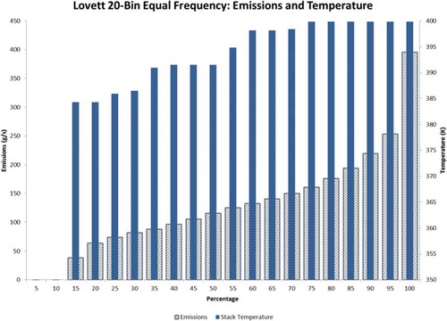
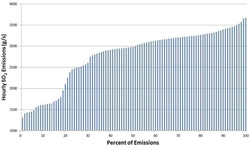
Lovett represented a complex terrain case with a single stack and nine ambient monitors with a full year of meteorological data. The frequency distribution of emissions used for Lovett is shown in Figure 3. For the emission bin distribution using equal frequencies of hours, we present the associated stack gas exit velocities in Figure 4 and the stack gas temperatures in Figure 5. The behavior of the exit velocities and temperatures among the cases is typical for a boiler, with increasing load being associated with higher emissions, higher air flow, and somewhat higher temperatures. Due to the similarity of the behavior of the stack exhaust parameters for the other evaluation databases, those additional figures are not included in this paper.

Figure 3. Frequency distribution of SO₂ emissions for Lovett (year 1988).

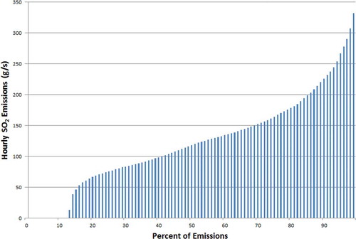
Figure 4. Exit velocities and SO₂ emissions for each Lovett bin.

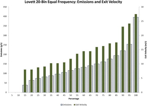
Figure 5. Stack gas exit temperatures and SO₂ emissions for each Lovett bin.

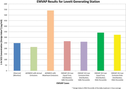
The 50th and 95th percentiles of the results from 1000 iterations of EMVAP were then compared to AERMOD run with actual hourly emissions as well as with peak hourly emissions. The comparison also included the observed design concentration (over all monitors). The results are shown in Figure 6, which shows, from left to right, the observed concentration at the monitors, the design concentration as predicted by AERMOD using actual hourly emissions as well as peak emissions, and then the EMVAP median (50th percentile) and 95th percentile design value concentrations from 1,000 iterations for the equal frequency and equal emission increment bins. The results shown in Figure 6 are as we expected: AERMOD with actual emissions shows good performance, AERMOD with constant peak emissions overpredicts substantially, and EMVAP results are somewhat more conservative relative to AERMOD with actual emissions. The level of conservatism varies with the selected percentile of the results over all iterations. It is important to keep in mind that the EMVAP results are expected to show higher design concentrations than the use of actual hourly emissions because (1) as explained earlier, the high emission hours are distributed over more days than they would be if clustering of high emissions was considered, so that the number of days with at least one high emission hour is maximized; and (2) the emission rate used for each “bin” is the maximum value in that bin (as shown in Figure 2), so that the weighted average of the emissions used by EMVAP is higher than the weighted average of the actual emissions.

Figure 6. Comparison of EMVAP results to monitored and AERMOD concentrations for Lovett.

Case 2: Clifty Creek

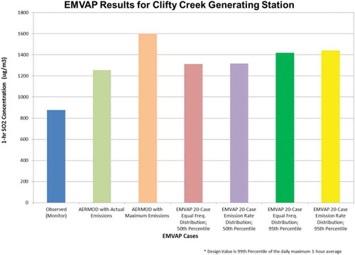
A second database included in the evaluation was Clifty Creek, located in the Ohio River Valley. This study included three units with varying load profiles, and six monitors. The emissions distribution for Clifty Creek Unit 1 is shown in Figure 7. The other two units, not shown here, had similar emissions distributions. In this case, the emission curves were somewhat flatter than that of Lovett Generating Station.

Figure 7. Frequency distribution of SO₂ emissions for Clifty Creek Unit 1 (year 1975).

EMVAP was again run in the two different ways described above for Lovett. The results of the EMVAP runs are shown in Figure 8. Although the results for Clifty Creek are qualitatively similar to those of Lovett, the flatter emissions distribution leads to the result that the EMVAP results for the design concentration are not as far below that for the peak emissions as was the case for Lovett, which had a steeper emissions distribution.

Figure 8. Comparison of EMVAP results to monitored and AERMOD concentrations for Clifty Creek.

Case 3: Kincaid

A third database evaluated involved the 1980–1981 SO₂ field study at the Kincaid Generating Station. The facility is located in a flat, rural area of Illinois. The study included 28 continuous SO₂ monitors, with about 7 months of data. The EMVAP load cases were then created using just those hours during which the experimental data were available. The emissions distribution for the Kincaid database is shown in Figure 9.

Figure 9. Frequency distribution of SO₂ emissions at Kincaid (1980–1981).

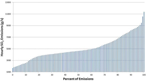
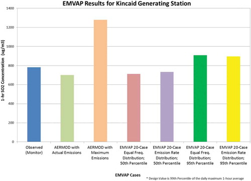
EMVAP was again run in the two ways as described for Lovett and Clifty Creek. The results of the EMVAP runs are shown in Figure 10. The comparison of EMVAP results to those for actual hourly emissions indicates that the 50th percentile shows about the same design concentration, while the 95th percentile EMVAP result is more conservative. For any given application, the authors recommend that a run of EMVAP should be conducted against modeling with actual hourly emissions to determine which ranked percentile over all of the EMVAP-generated simulated years shows a design concentration that is equal to or higher than the design concentration for the actual hourly emissions. Note that due to an uncertainty in the observed SO₂ concentrations due to a tolerance of up to 10% in differences found during calibration procedures (EPA, 2013), being “equal” for modeling can range from a predicted to observed ratio ranging from 0.9 to 1.1. In general, we recommend using a minimum 50th percentile because the form of the NAAQS is the average over all years tested.

Figure 10. Comparison of EMVAP results to monitored and AERMOD concentrations for Kincaid.

The basic goal of EMVAP is to provide a realistic, yet conservative (overpredictive), result for the modeled design concentration. The nature of the 1-hr SO₂ and NO₂ NAAQS is probabilistic, such that outliers that may occur with a simulated concurrence of worst-case meteorological conditions and worst-case emissions will be very infrequent. EMVAP provides a means to simulate these events with a prescribed emissions distribution and a series of meteorological conditions that make up the 1- to 5-year period actually simulated by AERMOD. Evaluation conducted so far has indicated that the results of EMVAP are fairly predictable and do not result in unexpected outcomes. It is understood that over many iterations, the extreme tails of the Monte Carlo distribution may be potentially unrealistic. For this reason, we have used the 50th percentile and 95th percentile EMVAP estimates in the evaluation results demonstration. Further testing by the modeling community is, of course, welcomed by the authors.

EMVAP Application for 30-Day Average Emission Rate

Conceptual approach

Previous EPA guidance, such as that issued by EPA (2011) for SO₂ implementation in September 2011, has recommended that averaging times in State Implementation Plan (SIP) emissions limits should not exceed the averaging time of the applicable NAAQS that the limit is intended to help attain. Following this approach would imply that emission limits for attaining the 1-hr SO₂ NAAQS should limit emissions based upon a single 1-hr limit, rather than limiting emissions that are averaged across a longer time period. This approach would assure that emissions in compliance with such a limit cannot result in a NAAQS violation. For purposes of discussion in the following, the term critical value refers to the highest constant hourly emission rate that would show compliance with the 1-hr SO₂ NAAQS with a modeling demonstration.

The EPA (2014b) noted in its SO₂ nonattainment modeling guidance that the requirement for a 1-hr emission limit might be too restrictive if short-term periods of emissions above the critical value were to have an extremely low likelihood of causing a NAAQS violation. This consideration is important for emission sources that have highly variable hourly emissions. The EPA addressed those concerns with recent guidance for 1-hr SO₂ nonattainment area State Implementation Plan submissions to allow for statistical techniques to accommodate the effect of infrequent high emissions. We evaluated this variability in short-term emissions in an example shown below by demonstrating that a longer-term average emission limit can still protect the 1-hr NAAQS. We note that EMVAP can be used as a statistical tool to demonstrate that rare occurrences of hourly emissions above the critical value would not threaten compliance with the 1-hr SO₂ NAAQS.

As a starting point in this process, we recommend, consistent with the 2014 EPA guidance, an initial modeling demonstration of the traditional type that sets the “critical value.” In the case of a single source with a defined background concentration, there is only one possible critical value. For multiple sources, it is possible to have multiple outcomes for critical values for each source modeled, but to simplify this EMVAP example, we have used a single isolated source. Consistent with the EPA guidance, we note that an emission rate for an averaging time longer than 1 hr would need to have a value that is no higher than the critical value, and EMVAP could be used to assure that the NAAQS is met with the assumed emissions distribution that can be used to set a longer term (e.g., 30-day) emission rate.

Example application

The general approach for the use of EMVAP to provide assurance that a 30-day average emission rate is protective of the 1-hour NAAQS is described below. The basic steps in the process are as follows:

• First, find the 1-hr average “critical value” with a traditional modeling approach.

• Then determine an emissions distribution that is applicable to the future operation.

• Next, set up EMVAP with the emissions distribution; EMVAP will use the emissions distribution and scale the modeling results to indicate a complying long-term emission rate value (e.g., a 30-day average).

• Run EMVAP to determine the complying emission rate (this will likely involve a reduced emission value relative to the critical value, as EPA expects to see).

• Rerun EMVAP with complying emissions (scaled) to verify NAAQS compliance, especially important if multiple sources are involved.

For estimating the emission distribution for future years, it is necessary to either use engineering judgment, for example, the applicability of emissions distributions from existing sources, or to obtain an actual sequence of hourly emission variations (and stack exhaust parameter variations) from an existing source that is expected to be a good match for the future source operation. This “emulation” of the future emissions distribution may require an adjustment to vary these parameters from an existing source to the future source of interest. We recommend that the EMVAP user should create an hourly sequence of future emissions that could then be used for input to EMDIST. Such a sequence could also be used to challenge EMVAP’s ability to predict at least as high as the modeled result with “actual” hourly emissions, and to establish the appropriate percentile level of the distribution of design values to select from the EMVAP run.

For this example case, we have used a single-stack source with the following stack exhaust parameters:

• Stack height: 122 m.

• Stack diameter: 5.2 m.

• Stack temperature: 416 K.

• Exit velocity: 23 m/sec.

We also assume for this example that the ambient SO₂ background concentration is 15 ppb (39.3 μg/m³). With standard AERMOD modeling in a flat terrain situation with 5 years of representative meteorological data, we find that an SO₂ emission rate of 327 g/sec shows compliance (by a small margin) with the 1-hr SO₂ NAAQS (196.5 μg/m³). Therefore, the outcome of the first step is the determination that the critical value emission rate is 327 g/sec. This emission rate, if realized on a continuous basis, would result in compliance with the 1-hr SO₂ NAAQS for the future stack operation.

For the determination of the emissions distribution to expect for the future operation of this source, assume that we have been provided with continuous emissions data from a similar source that is expected to be representative of the future operation of the source being modeled. Figure 11 shows a sample of the time series of actual SO₂ emissions from this representative source, and Figure 12 shows the depiction of the emission distribution to be used as input to EMVAP. The emission bins are such that they completely cover, with a safety margin, the cumulative distribution plotted from the representative source.

Figure 11. Time series of hourly emissions from representative source.

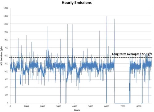
Figure 12. Emissions distribution for use in EMVAP.

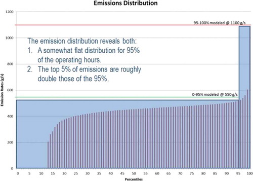
Note that for this example, the top 5% emission bin has an emission rate that is twice that of the remaining 95% time of operation. This type of distribution may be characteristic of base-loaded power plants with infrequent higher emissions associated with startup, shutdown, or maintenance/malfunction operations. For this example, assume that we have conducted a test of the EMVAP bins against actual hourly emissions with AERMOD and have determined that the selection of the 95th percentile result is sufficiently conservative. In other EMVAP applications, the selection of the 50th percentile result may be adequately conservative.

The next step involves the use of EMVAP with the same meteorological data and modeling approach that was used in the first step to obtain the “critical value” emission rate. For this step, however, AERMOD is run for each separate emission bin (there are two bins in this example), using the appropriate stack parameters and a 1-g/sec emission rate for these two bins. For this example, we assume the same stack parameters for the 95% bin and the 5% bin, but for other applications, it would be possible to have different stack exhaust parameters, or even different physical stack parameters or locations (such as for a bypass stack).

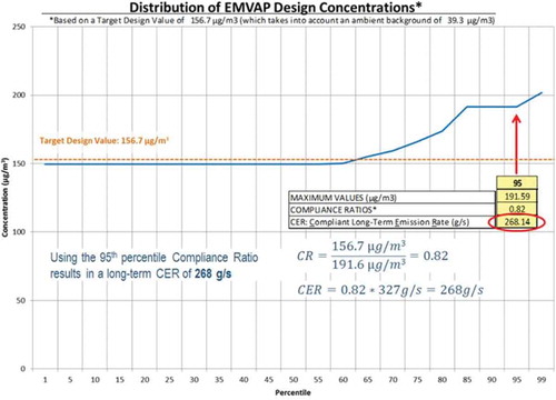
In this example, EMVAP presents a series of compliance ratios and associated long-term (30-day) emission rates depending upon the percentile of the results (over all 1,000 simulated years) that is selected, as shown in Figure 13. Note that for percentages of the EMVAP design concentrations up to about the 60th percentile, the long-term complying emission rate would be the same as the 1-hr critical value. However, with increasingly constraining percentiles, the complying long-term emission rate must be less than the 1-hr critical value. For the 95th percentile EMVAP result (which is the one selected for this example), the predicted design concentration (minus background) requires an emission reduction of 18% to show a result that barely complies with the NAAQS. Therefore, the long-term emission rate is 82% of the 1-hr critical value, or 268.14 g/sec.

Figure 13. Results of example EMVAP compliance emission rate analysis.

The last step in the process is to verify, through a final refined run of EMVAP, that the selected adjustments to the emission rate will show NAAQS compliance. In this case, the emission rates used as input to EMVAP for the Critical Value Analysis Option are scaled through an “adjustment factor” provided by the EMVAP Critical Value Analysis run so that the weighted average is the long-term complying emission rate. The result is as expected: The long-term emission rate is about 268.1 g/sec, comprised of an emission bin valid 95% of the time with an emission rate of about 255.4 g/sec and a bin valid 5% of the time with an emission rate twice as high (about 510.7 g/sec). For this final analysis, refinements or adjustments in the background component may require reruns of EMVAP with slight emission rate adjustments to show NAAQS compliance.

Conclusion

Due to stringent 1-hr SO₂ and NO₂ NAAQS, there is a need to account for variable emissions distributions to address these probabilistic NAAQS. To respond to this need, we have developed an advanced technique, the Emissions Variability Processor (EMVAP), which can account for emissions variability in dispersion modeling through Monte Carlo sampling of emission rates with user-specified emission frequency distributions. Based upon concentrations from 1 to 5 years of meteorological conditions as modeled by AERMOD, EMVAP as a postprocessing step can simulate hundreds or even thousands of years of randomly generated concentration predictions, from which the probabilistic distribution of the design concentrations can be generated.

This paper provides an overall description of the concept and design of the EMVAP model postprocessor. It shows through evaluation results on three separate databases that the 50th or 95th percentile predicted design concentrations from as many as a thousand simulated years are consistently equal to or higher than modeling using actual hourly emissions. Therefore, use of EMVAP can be relied upon to provide a statistically robust demonstration of compliance with the 1-hr NAAQS.

Previous EPA guidance had recommended that averaging times in State Implementation Plan emission limits should not exceed the averaging time of the applicable NAAQS that the limit is intended to help attain. However, new EPA guidance allows the use of the longer averaging time to address 1-hr limits that can accommodate infrequent high emission rates. We show that EMVAP can be used to make this demonstration, with the following steps:

• Conduct AERMOD modeling in the traditional sense with constant emissions to determine a “critical value” 1-hr emission limit that shows marginal NAAQS compliance.

• Define an emissions distribution that features a small percentage of emissions higher than the critical value and a weighted average that is at or below the critical value.

• Determine the percentile result for EMVAP that is sufficiently conservative by testing EMVAP against a time series of actual hourly emissions using AERMOD modeling.

• Show with EMVAP that this emissions distribution also shows NAAQS compliance.

We provide an example of an emissions distribution that illustrates how this approach would work in practice using EMVAP.

Additional information

Notes on contributors

Robert Paine

Robert Paine, CCM, QEP, is an associate vice president and technical director, Carlos Szembek is a software programmer and air quality meteorologist, and David Heinold, CCM, is a senior air quality meteorologist with AECOM’s Air Quality Modeling group in Chelmsford, MA.

Carlos Szembek

Robert Paine, CCM, QEP, is an associate vice president and technical director, Carlos Szembek is a software programmer and air quality meteorologist, and David Heinold, CCM, is a senior air quality meteorologist with AECOM’s Air Quality Modeling group in Chelmsford, MA.

David Heinold

Robert Paine, CCM, QEP, is an associate vice president and technical director, Carlos Szembek is a software programmer and air quality meteorologist, and David Heinold, CCM, is a senior air quality meteorologist with AECOM’s Air Quality Modeling group in Chelmsford, MA.

Eladio Knipping

Eladio Knipping is a principal technical leader in the Environment Sector at the Electric Power Research Institute office in Washington, DC.

Naresh Kumar

Naresh Kumar is a senior program manager of air quality in the environment sector at the Electric Power Research Institute office in Palo Alto, CA.

References

- Blewitt, D. 2011. Analysis of near field NO2 conversion rates and the development of a NO2 repartitioning modeling approach for demonstrating compliance with the 1-hour NO2 standard. Paper A-626, 104th Annual Conference and Exhibition of the Air & Waste Management Association, Orlando, FL. Air & Waste Management Association, Pittsburgh, PA.
- Cimorelli, A.J., S.G. Perry, A. Venkatram, J.C. Weil, R.J. Paine, R.B. Wilson, R.F. Lee, W.D. Peters, and R.W. Brode. 2005. AERMOD: A dispersion model for industrial source applications. Part I: General model formulation and boundary layer characterization. Journal of Applied Meteorology 44:682–693. doi:10.1175/JAM2227.1
- Cole, H.S., and J.E. Summerhays. 1979. A review of techniques available for estimating short-term NO2 concentrations. Journal of the Air Pollution Control Association 29(8): 812–817. doi:10.1080/00022470.1979.10470866
- Electric Power Research Institute (EPRI). 2014. EMVAP user manual, code, and test cases download web site. http://secourceforge.net/projects/epri-dispersion (accessed May 1, 2014).
- Hanrahan, P.L. 1999a. The plume volume molar ratio method for determining NO2/NOx ratios in modeling—Part I: Methodology. J. Air Waste Manage. Assoc. 49:1324–1331. doi:10.1080/10473289.1999.10463960
- Hanrahan, P.L. 1999b. The plume volume molar ratio method for determining NO2/NOx ratios in modeling—Part II: Evaluation studies. J. Air Waste Manage. Assoc. 49:1332–1338. doi:10.1080/10473289.1999.10463961
- Perry, S.G., A.J. Cimorelli, R.J. Paine, R.W. Brode, J.C. Weil, A. Venkatram, R.B. Wilson, R.F. Lee, and W.D. Peters. 2005. AERMOD: A dispersion model for industrial source applications. Part II: Model performance against 17 field study databases. J. Appl. Meteorol. 44:694–708. doi:10.1175/JAM2228.1
- Podrez, M. 2013. Ambient Ratio Method Version 2 (ARM2) for use with AERMOD 1-hr NO2 Modeling. Control #10. Presented at the A&WMA Specialty Conference: Guideline on Air Quality Models: The Path Forward, Raleigh, NC. Air & Waste Management Association, Pittsburgh, PA.
- U.S. Environmental Protection Agency. 2003. AERMOD: Latest features and evaluation results. http://www.epa.gov/ttn/scram/7thconf/aermod/aermod_mep.pdf (accessed May 1, 2014).
- U.S. Environmental Protection Agency. 2005. Appendix W to 40 CFR Part 41. Federal Register 70:68218. http://www.epa.gov/seccram001/guidance/guide/appw_05.pdf (accessed May 1, 2014).
- U.S. Environmental Protection Agency. 2011. Guidance for 1-hour SO2 NAAQS SIP submissions. http://www.epa.gov/airquality/seculfurdioxide/pdfs/DraftSO2Guidance_9-22-11.pdf (accessed May 1, 2014).
- U.S. Environmental Protection Agency. 2013. Quality Assurance Handbook for Air Pollution Measurement Systems, Volume II, Ambient Air Quality Monitoring Program, 2013. http://www.epa.gov/ttnamti1/files/ambient/pm25/qa/QA-Handbook-Vol-II.pdf (accessed June 15, 2014; see Table 10-3 and Appendix D, p. 13).
- U.S. Environmental Protection Agency. 2014a. SO2 NAAQS designations modeling technical assistance document. http://www.epa.gov/airquality/seculfurdioxide/implement.html (accessed May 1, 2014).
- U.S. Environmental Protection Agency. 2014b. Guidance for 1-hour SO2 nonattainment area SIP submissions. http://www.epa.gov/airquality/sulfurdioxide/pdfs/20140423guidance.pdf. (accessed May 1, 2014).
- U.S. Environmental Protection Agency. 2014c. NO2 modeling: Current status and plans for updates to Appendix W. http://www.cleanairinfo.com/regionalstatelocalmodelingworkshop/archive/2014/Presentations/Tues/015-Appendix%20W%20NO2%20updates%20RSL%202014_v2.pdf (accessed June 15, 2014).