Emission factors for fugitive dust from bulldozers working on a coal pile

Abstract

A study of a Powder River Basin (PRB) coal pile found that fugitive emissions from natural and human activity each produced similar levels of downwind fine + coarse (i.e., smaller than 10 µm, or PM₁₀) particle mass concentrations. Natural impacts were statistically removed from downwind measurements to estimate emission factor E_v for bulldozers working on the pile. The E_v determined here was similar in magnitude to emission factors (EFs) computed using a U.S. Environmental Protection Agency (EPA) formulation for unpaved surfaces at industrial sites, even though the latter was not based on data for coal piles. EF formulations from this study and those in the EPA guidance yield values of similar magnitude but differ in the variables used to compute E_v variations. EPA studies included effects of surface silt fraction and vehicle weight, while the present study captured the influence of coal moisture. Our data indicate that the relationship between PRB coal fugitive dust E_v (expressed as mass of PM₁₀ emitted per minute of bulldozer operation) and coal moisture content M_c (in percent) at the study site is best expressed as E_v =10^f(M_c) where f(M_c) is a function of moisture. This function was determined by statistical regression between log₁₀(E_v) and M_c where both E_v and M_c are expressed as daily averages of observations based on 289 hours sampled during 44 days from late June through mid-November of 2012. A methodology is described that estimates M_c based on available meteorological data (precipitation amount and solar radiation flux). An example is given of computed variations in daily E_v for an entire year. This illustrates the sensitivity of the daily average particulate EF to meteorological variability at one location. Finally, a method is suggested for combining the moisture-sensitive formulation for E_v with the EPA formulation to accommodate a larger number of independent variables that influence fugitive emissions.

Implications: Fugitive coal dust emission factors (EFs) derived by this study contribute to the small existing knowledge base for a type of pollutant that will become increasingly important as ambient particulate standards become tighter. In areas that are not in attainment with standards, realistic EFs can be used for compliance modeling and can help identify which classes of sources are best targeted to achieve desired air quality levels. Reconciling emission factor formulations that are sensitive to different factors (i.e., those from the EPA and this study) produces a more powerful tool for estimating fugitive emissions at a broad range of sources.

Introduction

Fugitive emissions are emitted gaseous or aerosol materials that do not pass through vents, stacks, or other openings. These emissions can affect air quality near a source and are regulated by federal and state agencies. By their nature, fugitive emissions are difficult to quantify. Indirect techniques have been used to estimate emissions and relate them to some kind of human activity or physical process. For example, Cowherd et al. (1974) employed a mass balance approach to derive fugitive dust emission rates from unpaved roads and other surfaces. The U.S. Environmental Protection Agency (EPA) has adopted emission factors (EFs) based on this method. Fugitive dust EFs for coal mining operations, developed using mass balance techniques, were reported by the EPA (1998). These EFs have been adopted by states and in other countries (e.g., Ghose, 2004). Unfortunately, there has been little original research published on fugitive coal dust EF development (other than the work for EPA) and there is a paucity of literature on the topic.

The mass balance method requires extensive monitoring upwind and downwind of a source to ensure that the majority of source emissions are detected. Successful application of this method requires that source attributes be reasonably constant during each monitoring period, that other sources not be present, and that all emitted mass be accurately detected. The method is not without its problems, though. In the case of particulate matter, the variable nature (and in some cases the size) of sources and the size distribution of emitted particles are factors that make it difficult to meet all these requirements. An additional problem occurs when the source is co-located at a site in close proximity to other sources whose emissions may confound measurements. In a summary of fugitive emissions data from construction activities, Muleski et al. (2005) note that vehicle exhaust is often a major contributor to PM_2.5 (i.e., airborne mass concentrations of particles with aerodynamic diameters <2.5 µm) emissions when measurements are made in close proximity to moving vehicles. The presence of stationary engines (such as cranes, power shovels, generators, etc.) or burning debris can complicate efforts to assign emissions to vehicles in motion. These issues often require that measurements be made at locations where activity is staged to eliminate undesirable interferences. Venkatram (2000) analyzed limitations associated with the empirical methods used to derive EF formulations like those used by the EPA, including the lack of a mechanistic basis and (as just mentioned) a dependence on the unique characteristics of the data sets from which they are derived. Given these limitations, there is adequate motivation to supplement purely empirical methods with alternate approaches to estimating EFs.

An alternate method for quantifying fugitive emissions is one in which ambient monitoring is combined with dispersion modeling. In this approach, ambient data are combined with detailed meteorological measurements and a model of pollutant transport and dispersion to compute downwind patterns of fugitive pollutants and back-calculate (i.e., inverse model) the source strength. This method was previously applied to estimate particulate EFs for roadways (Venkatram et al., 1999) and for a dry fly ash disposal operation (Mueller et al., 2013). In the latter study, the source area of fugitive particles covered roughly 8200 m² (0.8 ha) and the sampling was performed sufficiently far downwind that the fugitive dust plume had adequate time to grow large enough to frequently impact downwind monitors. This method eliminated anything artificial about sampling emissions from a staged activity and allowed study of a source that is rarely found anywhere except at an active coal-burning power plant. Even so, care was needed to identify confounding sources and to remove their contributions to ambient measurements.

Recently, a study was undertaken of fugitive dust from a pile of Powder River Basin (PRB) coal at an active power plant site following methods previously used by Mueller et al. (2013). The pile covered about 6.6 ha and its dimension perpendicular to the predominant wind directions (southwest and south-southwest) was about 380 m (see the next section for details). Monitors were located within 200 m downwind of this pile. Measurements collected thousands of hours of particulate and meteorological data near the pile plus video imagery in an effort to quantify fugitive dust emissions. In the present context, “dust” refers to particles smaller than 10 µm in size (PM₁₀). Previous studies have included particles larger than 10 µm but those particles are unlikely to be transported off-site and have little bearing on air regulatory compliance because current standards focus only on inhalable particulate matter (i.e., PM₁₀ and PM_2.5).

Enhanced particulate levels were measured downwind of the pile both with and without human activity on the pile. The primary human activity that produced fugitive dust was the movement of bulldozers across the coal surface, although coal was periodically dropped onto the pile from an overhead conveyor system. The latter activity was infrequent and hours when it occurred were not analyzed. Bulldozers worked to move coal between points on the pile and to scrape the coal surface. The latter activity was needed to suppress the spontaneous combustion of coal dust and is referred to here as “grooming.”

Quantifying coal dust fugitive emissions from bulldozer activity required that natural dust contributions to downwind concentrations be removed from the total observed concentrations. Natural dust emissions are described at length by Mueller et al. (2015) for this site. Their primary finding was that natural processes at the study site produced significant downwind particulate concentrations that could not be ignored when using ambient measurements to determine fugitive emissions from anthropogenic activity. This finding depended in part on knowledge of hourly bulldozer activity, which was documented using a camera. Dust transport and dispersion from the coal pile were subsequently simulated to identify the human-made dust impact. Estimated PM₁₀ emission rates and EFs due to bulldozer activity were then derived based on measured concentrations and observed coal pile activity. An upper limit was estimated for PM_2.5 emissions relative to PM₁₀. This paper summarizes the analysis used to estimate the EFs, compares results with those from previous work and provides an example of how the new EF formulation can be applied to a site using representative meteorological data.

Emissions Factor as Engineering Tool

The emissions factor E is an engineering tool to facilitate fugitive emissions estimates in terms of a more easily derived quantity. For example, fugitive dust emissions can be estimated for an unpaved road using a dust emissions factor expressed as mass of dust emitted per vehicle distance traveled. When multiplied by vehicle travel distance per unit time (such as an annual value) this factor yields a mass emission rate.

Emission factors are typically used when emission estimates are needed for air permit applications or when there is a requirement to explicitly model the downwind air quality impacts of a fugitive dust source. In many situations formulas for E do not exist for the type of source in question, requiring use of E formulations for other source types. The primary source of these formulations is the U.S. Environmental Protection Agency (EPA) AP-42 Emissions Handbook (EPA, 1995). AP-42 contains fugitive dust EF formulations for aggregate dropping operations and for vehicles driving on unpaved surfaces. In the case of bulldozers driving across a coal pile, the formulation for vehicles driving on unpaved roads at an industrial facility is the one most closely related:

(1)

In eq 1, s is the silt content (percent) of the surface, W is vehicle weight (short tons), and E_ir is the emission factor expressed as kilograms per vehicle distance (km) traveled for the ith particle size fraction. Constant k_i is a particle size fraction adjustment factor equal to 1.5 for the PM₁₀ size fraction. Exponent a = 0.9 for PM₁₀. Unlike the E formulation for unpaved public roads (EPA, 1995), eq 1 does not include corrections for surface moisture content or vehicle speed, probably because these factors were not well represented by the original experimental data. Also, eq 1 was not based on data from a coal pile. However, it is frequently applied to bulldozers driving on coal because AP-42 dos not contain alternate EF formulations. The coal surface is similar to other unpaved nonroad industrial surfaces because of infrequent traffic and less compaction and weathering than on public roads.

Coal piles exposed to varying weather conditions can have moderate or even large variations in surface moisture content in all but the driest climates. In addition, water spraying is one method used to control wind erosion from coal piles. Therefore, there is a need to derive a dust EF formulation for coal piles that considers the influence of moisture.

Emission Derivation

Measurements

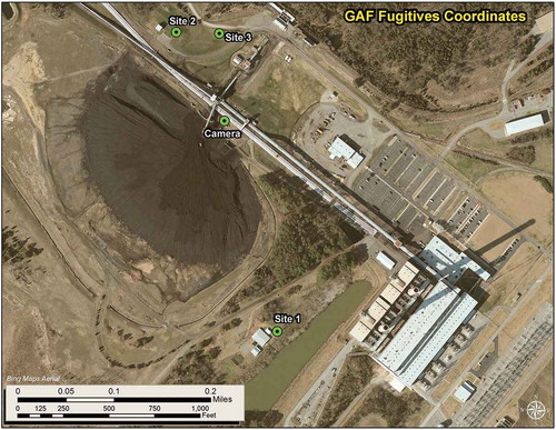
A study of fugitive dust emissions from a PRB coal pile was conducted at the Gallatin (Tennessee) electric power generating station during the summer and autumn of 2012. The area around the coal pile is shown in Figure 1. Beta attenuation monitors (BAMs) measured hourly PM₁₀ and PM_2.5 concentrations at sites labeled 1, 2, and 3 in the figure. The BAM measurement accuracy was ±4 µg m⁻³ (Mueller et al., 2013), whereas the instrumental precision was 1 µg m⁻³. Frequent southerly winds made site 1 the prevailing upwind site, while sites 2 and 3 were most often downwind. A 10-m meteorological tower near site 2 collected data on winds (three-dimensional sonic anemometers), temperature, and humidity at two levels (2.3 and 9.6 m) and net radiation. A nearby rain gauge, buried resistance sensor, and nephelometer collected data on precipitation, soil moisture content (at 5 cm below the surface), and light scattering at 525 nm. The latter measurement was useful in identifying at high-time-resolution (i.e., 1 min) plumes of particles smaller than about 1 µm. At sites 1 and 2, low-volume Federal Reference Method particle filter samplers collected PM₁₀ mass on Teflon and quartz filters for subsequent chemical analysis. The instrumentation used in this study was the same as that described by Mueller et al. (2013) for a previous study.

Figure 1. Environs surrounding the coal pile (oval black area) at the Tennessee study site. The photograph is oriented north-south from top to bottom. Monitoring sites are denoted by green circles.

A time-lapse camera (see Figure 1) with a 90-degree field of view lens imaged the coal pile and provided information on both human (e.g., bulldozers, other vehicles) and natural (e.g., dust devils, fires) activity at the pile. Site logs provided information on quantities of coal processed, along with the movement of coal through the handling system. On four separate occasions during the study coal samples were collected on the pile. These samples were later analyzed to determine silt and moisture content.

Separating contributions from different dust sources

The excess particulate concentration, C_xs, is defined in terms of the upwind and downwind concentrations:

(2)

Occurrences of the desired upwind–downwind configuration were determined by the 10-m wind direction. Winds from the south-southeast clockwise through west-southwest provide conditions when airflow passed over the coal pile and were sampled by monitors at sites 2 and 3. An additional adjustment was applied to normalize all concentrations by the fraction of time f airflow during an hour passed over the pile based on 1-min wind measurements. This adjusted concentration C_xs* was defined as

(3)

and provided a consistent measure of coal pile impact on downwind particulate levels across all hours. Note that values of f were >0 and ≤1 while averaging 0.71.

Average values of C_xs* for hours with and without human activity on the coal pile are summarized in Table 1. Concentrations in the presence of human activity (i.e., active bulldozers) were greater than concentrations without activity. The preponderance of nonzero C_xs* for hours without activity implies a “natural” source of particle emissions.

Table 1. Average adjusted PM₁₀ concentration C_xs* for hours without and with human activity on the coal pile

Monitoring site	Concentration, µg m^−3
	Without activity	With activity
2	19.7	60.7
3	21.1	59.9

Mueller et al. (2015) identified wind erosion and the action of microscale turbulence (a smaller scale form of wind erosion) on the coal pile as the most probable sources of natural fugitive emissions. AP-42 lists three different values for friction velocity (u*) erosion thresholds associated with coal: 0.55 m s⁻¹ for ground coal, 0.62 m s⁻¹ for scraper tracks on a coal pile, and 1.12 m s⁻¹ for an uncrusted coal pile. The present study used 0.55 m s⁻¹ as the lower limit (u_t*) for determining coal dust wind erosion at the study site. AP-42 indicates that wind is nearly 7 times more efficient at lofting particles in the PM₁₀ mass fraction compared to the PM_2.5 mass fraction for a given value of u*. Assuming a logarithmic wind speed profile, AP-42 suggests estimating the lowest short-term (i.e., ~1-min) surface wind speed u_s⁺ associated with particle erosion as

(4)

where the height of u_s⁺ is taken to be about 0.25 m above the surface. Wind tunnel studies have determined the ratio ρ_u = u_s/u₁₀ for different pile geometries and locations on such piles where u₁₀ is wind speed measured at a standard reference height of 10 m. AP-42 cites data suggesting ρ_u can be as high as 1.1 near the windward edges of pile tops. A 10-m wind speed threshold u_t (=minimum of u₁₀⁺) for erosion was estimated—rearranging eq 4 and inserting AP-42 values for minimum u_t* and maximum ρ_u—as

(5)

Thus, a potential was assumed to exist for wind-forced dust erosion on the coal pile whenever 1-min 10-m wind speeds were measured to be ≥5 m s⁻¹.

For hours when wind speed exceeded u_t, a statistical model provided a reliable method for calculating the natural fugitive dust concentration excess because it accounted for 70% of the variance in concentration. A model was also derived for early morning and evening hours when wind was below the erosion threshold.

Statistical models linking observed excess particulate concentration due to natural sources, , with site characteristics took the general form

(6)

µ = (u₁₀⁺ – u_t), σ_w is the standard deviation of the 10-m vertical wind component, T₂ is 2-m temperature, Γ₂ is 2-m relative humidity, is the 1-min maximum turbulent kinetic energy measured at 10 m, and d_a is the numerical day of the study (presumably this last predictor represents a surface conditioning effect that was not captured by any other parameter). Equation 6 was specific to each monitoring site. When winds were <u_t during hours before 9:00 a.m. or after 6:00 p.m. (referred to here as “stable hours”), a statistical model explained about 40% of the variance in concentration. Although not ideal, this model also provided guidance for estimating that had more skill than applying a single value such as a mean or median concentration. Thus, analogous to eq 6, the dependence of stable-hour was computed using

(7)

where x_m is the downwind distance from the pile edge to the monitor, x_f is the fetch across the pile (dependent on wind direction), t_h is the hour of the day, R_net is net radiation flux, ΔT = T₁₀ – T₂, and σ_u and σ_u⁺ are the standard deviation (hourly and 1-min maximum, respectively) of u₁₀. Both eqs 6 and 7 include information related to atmospheric transport and diffusion. In both formulations, predictors were selected that were significant with a confidence level >95%.

Statistically estimated values were constrained to be no more than the 95th percentile value observed during nonactivity hours to minimize the risk of overestimating natural dust contributions. During midday hours with low wind speeds (i.e., below the wind erosion threshold) for which no statistical model was available, median hourly values of for each hour from 9:00 a.m. through 6:00 p.m. were applied to hours with pile activity (values ranged from 25 to 34 µg m⁻³). All estimates of were subtracted from C_xs* to estimate PM₁₀ concentrations attributable to human activity, :

(8)

Table 2 summarizes the values of each of these variables for the hours when human activity was observed on the coal pile. No bulldozer activity occurred before 8:00 a.m. (i.e., the time period experiencing the lowest amount of natural emissions). Consequently, most hours experiencing bulldozer activity coincide with the midday maximum for natural emissions or the late afternoon/evening period when higher wind speeds made it more likely that wind erosion contributed to dust emissions from the pile (Mueller et al., 2015). The highest observed PM₁₀ concentrations were near or above 1000 µg m⁻³ and were typically associated with bulldozer activity. However, during most hours dust levels associated with natural emissions were not much different from levels occurring in the presence of bulldozer work. After removing the natural contribution from downwind measurements, a frequency distribution was obtained for human-derived dust levels that was strongly skewed toward low values. This is reflected in the low median and geometric mean values for compared to C_xs*.

Table 2. Comparison of fugitive PM₁₀ concentrations^a associated with natural and human activity on a coal pile (data from both downwind sites combined)

Variable	PM10 concentration statistic, µg m^−3
	Maximum	Mean	Median	Geometric mean
Cxs*	1196	60.3	33.1	33.8
	130	40.8	36.5	34.2
	1066	31.2	2.6	5.3

Note: ^aConcentrations were adjusted to reflect levels associated with continuous airflow over the source.

Frequency distributions of C_xs*, and are illustrated in Figure 2 for hours when winds transported dust from the pile toward downwind monitors. Concentration values from sites 2 and 3 were so similar that data for each variable were combined into joint distribution plots. Values of C_xs* were very skewed, ranging up to 1196 µg m⁻³ with a mean value of 60 µg m⁻³ and a median value of 33 µg m⁻³. By comparison, estimated values of ranged as high as 130 µg m⁻³ with mean and median values of 41 and 36 µg m⁻³, respectively. The distribution of is not nearly as skewed as that of C_xs*, in part because of the artificial 95th percentile constraint. However, the cap on is justified because of uncertainty in estimating it and the desire to not underestimate . Subtracting the two distributions produces a strongly skewed distribution for with maximum, mean, and median values of 1066, 31, and 3 µg m⁻³, respectively. This distribution (Figure 2) appears lognormal and is similar to that derived by Mueller et al. (2013) downwind of a fly ash disposal site. Thus, the geometric mean of —probably the most appropriate metric for describing these data—was 5.3 µg m⁻³. Note that constraints placed on hourly estimates of —as derived from eq 8—influenced values at the low end of the distribution. These factors are described in the next section.

Figure 2. Frequency distributions of C_xs* (top), (middle), and (bottom) for hours when airflow transported bulldozer-derived dust from the coal pile toward downwind monitors. Bin labels indicate the midpoint of each 20-µg m⁻³ range in bin values.

Inverse modeling to derive fugitive emission rates

Average concentration (mass per unit volume) of material emitted from a source at rate Q (mass per unit time) is related to the rate by

(9)

where is the time-average dispersion function (units of time per unit volume) that describes the dilution and spatial distribution of particulate matter in the air. In its most basic form,

(10)

for a Gaussian-shaped plume (u, y, z, σ_y, σ_z, and h denote wind speed, lateral offset from the plume centerline, height above ground, standard deviations of the concentration length scales [shape factors] along the y and z axes, and plume centerline height, respectively). All variables except u have units of length. Variants on this equation are used depending on specific atmospheric conditions that may restrict the dispersion of plume material. If Q is assumed to be constant during the averaging period,

(11)

If is taken to be the observed hourly concentration, then must be computed as the corresponding average dispersion function by using hourly meteorological parameters or by averaging results from sub-hourly periods. An alternate way to estimate Q is to replace with , which has essentially been averaged for the sub-hourly period when winds were observed blowing across the coal pile. In this approach, is modeled using only the meteorological conditions occurring when the airflow was across the pile.

Coal dust transport and dispersion was simulated using the EPA AERMOD model (EPA, 2004) and dividing the pile into three direction sectors, each with two subsectors “a” and “b” (Figure 3). The direction sectors were each about 30° wide and aligned approximately with the downwind monitoring sites. Table 3 lists the frequencies associated with airflow across each sector toward sites 2 and 3 along with the observed frequency of bulldozer activity inside each subsector for the hours modeled. Airflow and bulldozer activity were most frequent in sector 1 and least frequent for sector 3. Thus, most dust impacting the monitoring sites originated in sector 1.

Figure 3. Coal pile direction sectors (numbered 1 through 3) and subsectors (labeled “a” and “b” within each direction sector) for which hourly bulldozer activity was quantified by use of camera imagery. The camera was initially oriented to acquire images within the yellow-delineated field of view but was adjusted (red delineation) to capture a more central field of view—and more of sector 3—in September.

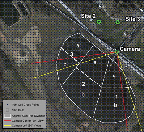
Table 3. Average observed frequencies (weights) used to allocate simulated fugitive dust emissions to each coal pile sector

Frequency	Downwind site	Coal pile sector
		1a	1b	2a	2b	3a	3b
Airflow across pile^a	2	0.35		0.27		0.19
	3	0.41		0.18		0.15
Pile activity^b	—	0.41	0.31	0.10	0.14	0.02	0.01
Airflow × activity^c	2	0.42	0.28	0.10	0.14	0.05	0.01
	3	0.45	0.29	0.10	0.11	0.03	0.01

Notes: ^aAverage frequency during each hour that the observed 1-min 10-m wind aligned a 30° coal-pile direction sector with a downwind site. Values in this row do not sum to 1.00 because of the minutes when airflow did not cross the pile (off-pile frequencies were 0.19 for site 2 and 0.26 for site 3).

^bObserved frequency of total hourly bulldozer activity that occurred within a coal pile sector. Row does not sum to 1.00 due to rounding.

^cJoint frequency of airflow and pile activity occurring relative to a downwind monitor. Rows may not sum to 1.00 due to rounding.

Table 4 summarizes sector-averaged meteorological parameters that controlled simulated coal dust transport and diffusion. The parameters (all measured at 10 m) are wind speed and direction (u₁₀ and θ₁₀), the standard deviation of θ₁₀ (σ_θ), the standard deviation of vertical wind speed w (σ_w), and turbulent kinetic energy (TKE). Parameter averages were determined only for those 1-min periods during an hour when sector and monitor were aligned (to within ±15°) as determined by the 10-m wind direction. Wind speed in the sectors having the highest values averaged 4–8% more than speed in the sectors having the lowest. Vertical turbulence, represented by σ_w, averaged 13% higher for the middle sectors than for the lateral sectors. Overall, sector differences translated into values of TKE that averaged 15% more in the middle sectors compared with the flanking sectors. Higher TKE implies more dispersion for dust emitted from the middle sectors.

Table 4. Sector-specific meteorological conditions at 10 m averaged for periods when airflow over the coal pile aligned with downwind monitoring sites

Site: sector	θ10 (deg.)	σθ (deg.)	u10 (m s^−1)	σw (m s^−1)	TKE^a (m^2 s^−2)
2: 1	168	15.4	1.66	0.28	0.19
2: 2	195	17.2	1.80	0.33	0.23
2: 3	228	17.3	1.74	0.31	0.20
3: 1	179	15.6	1.77	0.30	0.20
3: 2	208	18.5	1.71	0.34	0.23
3: 3	238	16.8	1.71	0.30	0.19

Note: ^aPer unit mass.

The sector-specific (i.e., based on sector-specific meteorology) dispersion function is denoted and when combined with the adjusted concentration yields

(13)

The advantage to using (i.e., the concentration normalized by f) is that it is more directly related to meteorological conditions over the dust source and this facilitates statistical modeling against other parameters. Likewise, using facilitates a modeling focus on only those conditions relevant to dust transport between the pile and the monitoring site. This approach assumes that the dispersion of coal pile dust during periods when the wind did not cross the pile did not significantly impact monitored concentrations. The close proximity of the monitoring sites to the source helped with this assumption because the emitted dust was transported to the monitors quickly (40–75 sec, on average), even when wind speeds were low. Although nonstationary winds could transport dust along a nonlinear path toward the monitors, any contribution to sampled air in these situations was assumed to be much smaller than the contribution of dust transported directly from the source to the monitors.

The largest potential for modeling error was when wind speed was intermittent, allowing airborne dust to accumulate over the pile during wind lulls and then transporting dust downwind when winds increased and aligned with the monitors. However, this nonsteady condition violates the steady-state assumption in AERMOD, so there is little expectation that averaging out these periods over an hour would do a better job of representing the dispersion function than limiting the modeling to those subhourly periods when the airflow aligned the source and monitors. This reasoning was the basis for modeling the dispersion function using subhourly meteorological data for minutes when source and monitor were aligned.

The six coal-pile subsectors were each assigned a weight ω_j based on the combined frequency of airflow and human activity. Polygonal areas representing each subsector were input to AERMOD and dust emissions were modeled as an area source. This approach facilitated computing Q because it allowed us to weight for the jth subsector according to the frequency with which airflow was aligned with a sector and the frequency with which human activity occurred within each source region during each hour. The particulate emission rate was computed from model results as

(14)

Table 5 lists source characteristics used to model dust emissions from each coal-pile subsector. Subsectors ranged in size from about a half hectare to just over 1 hectare. Only subsector 3b was totally elevated above the pile base. In subsectors 1a and 2a the elevation variation was assumed to be zero such that the initial depth of the dust plume was assumed to roughly equal the vehicle height consistent with camera observations. Bulldozers were required to move vertically while working within sectors in which elevation varied, and this created initial dust plumes with depths roughly equal to the change in elevation. Mean dust transport distances to the monitoring sites ranged between 214 and 306 m for subsectors 1a and 1b, which experienced the most bulldozer activity.

Table 5. Source characteristics used to model area emissions from the coal pile

Characteristic	Pile sector
	1a	1b	2a	2b	3a	3b
Area (ha)	0.72	1.15	1.09	1.09	0.69	0.46
Mean source elevation^a (m)	0	0	0	0	0	15
Initial plume depth^b (m)	2	15	2	15	12	2
Distance (m) from sector center to site 2	225	306	170	265	146	207
Distance (m) from sector center to site 3	214	299	187	285	214	255

Notes: ^aHeight relative to pile base.

^bThe minimum depth was roughly the height of the bulldozer. Larger values were selected to model dispersion from sectors in which the variation in pile elevation caused bulldozers to drive from lower to higher points on the pile.

Given the variability in both natural and human dust emissions, it was not surprising that hours occurred when ≥ C_xs*. In these cases,

(15)

This formula serves two purposes. First, when estimated > C_xs*, 4 µg m⁻³ is added to the difference to account for potential concentration measurement uncertainty (Mueller et al., 2013) that can produce slightly negative values after removing the estimated natural background. Second, eq 15 tests the estimated value of to ensure that, at a minimum, it had the lowest detectable value (1 µg m⁻³) reported by the BAM when pile activity was observed. Thus, a minimum value was assigned to equal to the lowest detectable value of C_xs* for hours when the human activity signal from the coal pile was low but within the combined noise of the PM₁₀ measurement and the estimate of . This adjustment was made in 35% of the hours analyzed and in most cases was probably necessary because of the small level of human activity on the pile during some hours (Figure 4). Observed bulldozer activity was ≤30 minutes for just over 20% of the hours studied, whereas the upper limit was 120 activity minutes (i.e., 2 bulldozers each operating for the full 60 minutes of an hour). This approach produces a conservative EF estimate because it ensures that at low levels of activity a nonzero estimate of emissions is computed. Conservatism in estimating emissions is desirable to protect public health and obtain regulatory acceptance.

Figure 4. Distribution of observed bulldozer activity (total minutes) per hour. Bin labels are the upper end of the 10-min range in bin values with up to two bulldozers working at once.

Computing PM₁₀ emission factors

The PM₁₀ fugitive particulate emission flux (mass per unit area per unit time, Q_f10 = Q/A where A is the source area) of coal dust produced by bulldozers operating on the coal pile was calculated from and the total simulated emission rate attributable to all six pile sectors weighted using the joint wind direction and activity frequencies determined for each sector. Table 6 summarizes Q_f10 and several other related particulate fluxes and emission rates. The mean values were skewed because of a small number of high values, so the median values are also provided because they better represent the central tendency of the derived emission flux distributions. The mean values are more than a factor of 10 greater than the medians.

Table 6. Calculated nonzero PM₁₀ coal dust emission rates due to bulldozer activity

Metric	Site 2	Site 3
Sample size	139	150
Mean Qf10, g ha^−1 sec^−1	5.5	3.2
Median Qf10, g ha^−1 sec^−1	0.09	0.10
Median Qe, kg hr^−1	0.76	0.71
Median Ev, kg min^−1	0.016	0.022
Geometric mean Ev, kg min^−1	0.026^a
AP-42 Ev from mean S, kg min^−1	0.121^a
Geometric mean of AP-42 Ev, kg min^−1	0.131^a

Note: ^aData from both downwind sites combined.

The mass emission rate Q_e represents the emitted mass per hour computed as

(16)

where q_j is the emission flux (mass per unit area per second) for the jth pile subsector and A_j is the corresponding subsector area. Emission rate distributions were computed using data from each downwind monitoring site. Distribution medians of both Q_f10 (= Σq_j/6, the average of q_j over the six pile subsectors) and Q_e are nearly the same for the two sites. Thus, results based on different monitoring data and slightly different mixes of meteorological conditions and pile sectors were quite similar. [Note: Using data from sites 2 and 3 separately, 10th percentile Q_e values were 0.09 and 0.10 kg hr⁻¹ (0.20 and 0.22 pounds hr⁻¹), respectively, and 90th percentile values were 18 and 33 kg hr⁻¹ (40 and 73 pounds hr⁻¹), respectively.] This similarity also exists for the mass emission rate per unit time of bulldozer operation given by

(17)

where t_v is the total minutes of bulldozer activity per hour. E_v data from both downwind sites were combined into a single data set. The distribution of E_v is essentially lognormal, consistent with .

One way to evaluate E_v is to compare its geometric mean with equivalent values computed using the AP-42 formula for the PM₁₀ fugitive EF (mass per distance traveled) for unpaved surfaces at an industrial site (i.e., eq 1). The mean observed s = 5% for the PRB coal with a range of 3.2–9.7%. A geometric mean of AP-42 E_v (note: E_v = VE_ir) of about 0.13 kg per minute (0.29 pounds min⁻¹) for bulldozer operations was computed using the observed distribution of s and assuming a mean vehicle speed V = 8 km hr⁻¹ (5 miles hr⁻¹). The EF based on the mean s was slightly lower at about 0.12 kg min⁻¹ (0.26 pounds min⁻¹). This compares (Table 6) to the geometric mean E_v from field data analysis of about 0.03 kg min⁻¹ (0.07 pounds min⁻¹).

Hourly 10-m wind direction indicated airflow across the coal pile (i.e., f > 0) in the absence of precipitation during 177 hours for site 2 and 178 hours for site 3 without human activity seen on the pile and with valid concentration data. Dust dispersion was simulated for all hours when subhourly (1-min) 10-m wind direction aligned a portion of the pile with the downwind monitors. For some hours there were no subhourly winds that aligned the pile and the monitors. This happened because the hourly wind direction was a resultant vector that was occasionally derived from winds blowing from directions on either side of the coal pile but not over the pile. No basis existed for computing dust plumes moving toward sites 2 and 3 without observing subhourly airflow across the pile. A small number of hours that were modeled produced no nonzero dust concentrations at sites 2 or 3. This was likely caused by winds that blew across the edge of the pile and, under stable conditions with little dispersion, did not produce plumes that were sufficiently wide to impact sites 2 or 3. Consequently, there were 38 hours at site 2 and 40 hours at site 3 when no plume impacts at the monitors were computed. The remaining joint (sites 2 and 3) data set contained 277 hours with valid, nonzero dust EFs.

Regarding a PM_2.5 E_v

The database was examined for evidence that human activity on the coal pile generated PM_2.5 emissions along with PM₁₀. The ratio of [PM_2.5]/[PM₁₀] was 0.14 when bulldozers operated, compared to 0.33 in the absence of human activity. The large decrease when human actions and natural erosion are mixed implies that the ratio due only to human activity is <0.14. Analysis showed that [PM₁₀] and [PM₁₀] were roughly equal for hours when human activity was present based on statistical estimates of the natural component. Observed natural PM₁₀ levels were only one-third of PM₁₀ measured in the presence of human activity (Table 1), although these data represent different sets of hours. It is likely that the actual ratio of natural to human-derived PM₁₀ was between one-third and one-half. Combining natural particulate levels (having a PM_2.5 mass fraction of 0.33) with human-influenced levels (having an unknown fraction of PM_2.5) must produce a net ratio :

(18)

In eq 18, F_hum and F_nat denote the fraction of total PM₁₀ associated with human and natural processes and must sum to 1. Variables and denote PM_2.5/PM₁₀ fractions that are associated with human and natural processes, respectively. must be slightly negative because = 0.33 and F_hum ≈ F_nat ≈ 0.50. Of course, a fraction <0 is impossible but—given uncertainty in F_hum and F_nat—this slightly negative result is not surprising. Alternatively, assuming F_nat = 0.33 and F_hum = 0.67 as shown in Table 1, then one must conclude = 0.045. These variations on estimating F_2.5(h) lead to the conclusion that 0 ≤ ≤ 0.045.

This demonstrates that human activity on the pile produces less PM_2.5 than natural processes. Comparing the two measured mass size fractions for the same hours revealed a small (r² < 0.2) linear correlation with confidence exceeding 99% that the slope m (as in the equation PM_2.5 = m PM₁₀ + b) was not zero (i.e., m = 0.06). Because natural processes did not show a significant relationship between the two size fractions, this result suggests that some small amount (~6%) of PM_2.5 is emitted from human-made actions on the pile. Given that this comparison uses data that include both natural and anthropogenic contributions to airborne particles, it is possible that a greater correlation exists between the two size fractions than is indicated from analysis.

These estimates of (from 0 to 0.06) are smaller than the ratio of 0.10 cited in AP-42 for fugitive particulate emissions associated with vehicle movement on unpaved industrial surfaces. The AP-42 value was not derived from tests of vehicles driving on crushed coal so its applicability is questionable. An upper limit of 0.06 is a conservative value to use based on the data presented here and would be consistent with results described for some western U.S. fugitive dust sources (Western Regional Air Partnership [WRAP], 2005).

Meteorological Variability

Derivation of PM₁₀ E_v formula

It is important to know what drives the variation in E_v so that these results can be applied for maximum accuracy. The first step is computing daily averages of log₁₀(E_v), denoted E_v^τ. The logarithmic transformation is needed to prevent extremely high values from controlling the results. Several potential predictors of E_v^τ were explored (e.g., temperature, wind speed, solar radiation flux, turbulence intensity, time spent by machinery driving on pile, bulldozer behaviors), but the strongest candidate was M_c. Coal moisture content can be measured from coal samples by comparing sample weights before and after oven drying. The loss in weight is attributable to water and is used to calculate M_c, usually expressed as a percent. This sampling could not be done all the time so a surrogate method was needed to determine M_c. It is likely that soil moisture content, M_s, is a suitable surrogate for M_c because both soil and crushed PRB coal contain particles of similar sizes and share some similarities in hygroscopic chemical constituents (e.g., calcium and other salts and metal oxides). Soil moisture content was measured adjacent to the meteorological tower using an electronic sensor buried roughly 5 cm below the soil surface. Twenty-four coal samples collected on four separate days were analyzed for M_c. Daily average standard deviations of measured M_c were only 2.4%, similar to that for M_s during corresponding rain-free periods. Daily average M_c and M_s were compared and found to share 85% of their variance. The resulting regression equation, (both M_s and M_c expressed as percent), was the basis for values of M_c used in subsequent analyses.

An investigation of soil moisture M_s and environmental factors was made to identify a means of estimating coal moisture content M_c using readily available data. Surface moisture levels result from a balance between water inputs (primarily precipitation) and losses (runoff and evapotranspiration). Runoff is highly variable, is greatest during and immediately following precipitation, and essentially falls to zero after prolonged periods without precipitation. Our soil monitoring site was flat (as was the sampling location for obtaining coal for water content analysis), implying that runoff toward and away from the measurement location was usually slow. Runoff can be neglected because it is likely to be infrequently affected by factors that control evapotranspiration on a 24-hr time scale. Therefore, to statistically analyze daily M_s variability, it is useful to assume that

(19)

where P is precipitation and e is evapotranspiration. Precipitation was directly measured. The water evaporation flux e is controlled by the rate at which water vapor is transported through the air layer above the ground. Following diffusion theory,

(20)

where ρ is the density of moist air, K_w is the eddy diffusivity for water vapor (unit area per unit time), and is the vertical gradient in specific humidity q_v (mass of water vapor per unit mass of moist air). It follows that q_v and its vertical gradient depend on air temperature T and solar radiation incident on the ground R_sol because, to a good approximation,

(21)

with saturation vapor pressure p_vs (at temperature T), air pressure p and relative humidity Γ. At the ground, T and Γ vary with T_s (surface temperature), R_sol, and M_s. Saturation vapor pressure increases with T, which implies a steeper gradient in q_v just above the surface and greater evaporation potential as T_s and R_sol increase. Hence, there is an expectation that M_s will vary negatively with T and R_sol, and positively with P.

This is exactly what was found when daily average M_s () was treated as the dependent variable in a multivariate linear statistical regression against the suite of observed meteorological variables. The only meteorological variables found to be significantly correlated with were daily average 2-m T (), daily average hourly R_sol (), and P₂₄ (24-hr precipitation amount). A similar statistical analysis of hourly M_s also indicated a dependence on wind speed but this dependence was not found for daily data.

During the 5-month (June–November) Gallatin coal pile study, more than half the variance in was associated with variance in and P₂₄, with only a minor amount tied to . However, to derive a more generalized statistical model of , a year of data collected previously at a different site in Alabama was included in our analysis. Inclusion of winter months increased the statistical importance of (presumably because days were included with very low solar input) but still resulted in a regression model that included the same three predictors identified from the Gallatin data set. This model of the combined data set explained about half the total variance in the daily average . However, an even better model was derived when from the previous day was included as a predictor. This is because of the high autocorrelation of with time-lagged values of itself. In such a model, 1-day lagged accounts for more than 70% of the variance in today’s , while and P₂₄ combine to account for an additional 14%. In this model solar radiation and precipitation serve as surrogates for soil (and coal) drying or moistening over the most recent 24-hr period while day-lagged adds a time-integrated influence (including the effect of past temperature) to the prediction equation that is not included in the previous model based on same-day data. The result is a formulation for that, when applied to an entire year of data, better replicates the observed daily variation in moisture content. Application of this method requires an initial guess of but the influence of the initial guess disappears after only a couple days of calculations. Initial values of should be in the range typical for PRB coal: between 15 and 35%.

The following formulation is based on data from a wide range of meteorological and seasonal conditions encompassing 361 days at two sites (total r² = 0.84):

(22)

In eq 22, each predictor of was determined to be significant with a confidence level exceeding 99%. With 1-day lagged expressed in percent, P₂₄ expressed in cm, and in W m⁻², the values of the coefficients were found to be a₀ = 8.17, a₁ = 0.761, a₂ = –0.013 W⁻¹ m², and a₃ = 0.553 cm⁻¹.

Analysis of E_v^τ was based on daily average values (to reduce data noise) compared with corresponding averages of other variables, including M_c and R_sol. Vehicle weight and speed were constant or nearly so and did not provide good predictors. The resulting data set contained 44 sets of values. Multivariate modeling of E_v^τ identified only one predictor, M_c, with statistical confidence at >99%.

The study was divided into two periods distinguished by whether routine coal removal (reclamation) from the pile was occurring. Exclusive reclamation began October 15 and continued through the end of the study. Ninety-five percent of the coal added to the pile during the study was added before August 9 and no coal additions were made after October 7. Of the coal removed from the pile, 70% occurred after October 15. Thus, before October 15, work on the pile was mostly focused on suppressing coal dust combustion (coal removal occurred sporadically on 30 of 107 days during this period). Coal surface grooming, occurring less than 8 hr/day, involved a bulldozer scraping its blade across the top of the coal to mix the top layer with underlying coal containing higher moisture content. Beginning October 15, bulldozers worked daily (12+ hours on some days) pushing coal toward an underground hopper for conveyance to the plant. During reclamation, bulldozers also continually reshaped the pile as coal was removed and this involved more pushing of surface coal.

A statistical comparison was made of E_v^τ with M_c for the two different periods. Results are illustrated in Figure 5. There is a clear negative association between E_v^τ and M_c that is different for each period. The regression for each period captures about half (46–52%) of the variance in E_v^τ. The remaining variability is due to measurement and modeling error, uncertainty in the correction to remove the natural dust component, and unknown variations in M_c across different portions of the pile. Regression slopes for the two periods are different, with less sensitivity to M_c and much higher values of E_v during the drier period. This difference could be influenced by the nature of the bulldozer work as previously described but the operational differences are subtle at best. The difference is more likely attributed to a seasonal effect driven by the drying capacity of the atmosphere. The cooler autumn period means less drying of the coal surface and higher M_c. The tendency for E_v^τ to decline more quickly as M_c increases is probably independent of season and bulldozer mode of action. Subbituminous coal becomes “sticky” (i.e., poses handling problems) with high moisture content. This change in physical characteristic—observed firsthand when taking coal samples for analysis—is likely the reason for the faster decline in E_v with increasing M_c because “sticky” coal has higher cohesive forces binding particles together. Note that the crushed coal has the consistency of wet concrete for M_c > 30%.

Figure 5. Plot compares daily average log₁₀(E_v) versus M_c for separate periods either ending before or beginning on October 15. Separate linear regression lines (and coefficients of determination) are shown for each period. The two lines intersect at roughly M_c = 29.5%.

Daily average values of E_v^τ versus M_c were alternately fitted with different regression curves (i.e., linear and polynomial formulations for M_c), but none provided a more satisfactory fit than those illustrated in Figure 5. Given the differences in the two data subsets previously described, it is recommended that either one or two linear regression formulas be used depending on circumstances. There is little data to support the E_v^τ extrapolated behavior at the extremes of M_c so caution is advised. A single formulation would be most appropriate in situations where M_c is always <30% (i.e., the “Before” data set regression in Figure 5). This is because the two linear equations shown in Figure 5 intersect at M_c ≈ 29.5%. For M_c > 30% the second formulation (the “After” data set regression in Figure 5) would be better because it reflects what is expected to be a rapid decline in E_v as the coal pile takes on a change in physical attribute. Thus, for M_c <29.5%,

(23)

with M_c expressed as a percentage. Constant c₁ was 689 kg min⁻¹ (1519 pounds min⁻¹). Note that PRB coal—the type studied here—tends to maintain high moisture content so that M_c values below 15% are unlikely (USGS, 1999). When M_c > 29.5% the best formulation is

(24)

In eq 24 c₂= 1.07 x 10¹¹ kg min⁻¹ (2.36 x 10¹¹ lb min⁻¹). Beware that eq 24 would greatly overestimate E_v for low M_c. At M_c = 29.5, eq 23 yields E_v = 0.023 kg min⁻¹ and eq 24 yields E_v = 0.027 kg min⁻¹ (the two equations intersect precisely at M_c = 29.786). For applications where a single formulation is most convenient, the following (regression r² = 0.52) is applicable across a larger range in M_c (but E_v overestimates at high M_c may be a problem):

(25)

with c₃ = 3175 kg min⁻¹ (7000 lb min⁻¹). Using eq 25, the dust EF essentially goes to zero (i.e., <1 g min⁻¹) for M_c >37%, although no data were collected for M_c this high.

Figure 6 compares E_v (using eqs 23 and 24) with E_v derived from V∙E_ir (denoted E_v(AP)) based on typical conditions for bulldozers operating on the PRB coal pile (s = 5%; W = 66 tons; V = 8 km hr⁻¹) and eq 1. The formula for E_ir does not include a variation with surface moisture so it is a constant 104 g min⁻¹ in the plot (the likely range in E_v(AP) due to s and V variability is also illustrated). On average, E_v > E_v(AP) for M_c < 25%. This comparison suggests that a very dry surface of PRB coal is capable of emitting PM₁₀ at a rate above that indicated by E_v(AP) for dry surfaces. However, the emission rate drops quickly and becomes negligible for moist surfaces. For reference, Figure 6 also shows the AP-42 moisture-dependent EF for unpaved public roads, assuming the same bulldozer speed and surface conditions as the coal pile. This formulation is not applicable to bulldozer work on coal piles but is shown here as a point of reference to illustrate the expected lower limit of fugitive emissions from surfaces that emit a lot less dust because of frequent use and compacted surfaces. The next section describes an example of how to apply this method for estimating and daily average E_v () from standard meteorological data.

Figure 6. Comparison of different values of E_v versus M_c using emission factors from AP-42 for unpaved public roads, unpaved industrial surfaces, and from this study. The potential variability of the E_v(AP) for industrial sites—assuming 25% variability in vehicle speed and surface silt content—is illustrated using dashed lines above and below the parallel solid line.

Application of E_v formula

Application of the coal dust EF E_v formulation is illustrated here using data collected by the National Weather Service (NWS) in Nashville, TN (temperature and precipitation), and in Bowling Green, KY (solar radiation). Nashville measurements are made a little more than 30 km southwest of the study site, whereas solar radiation data were collected about 65 km north of the site.

A time-series plot of daily average based on actual meteorological data is presented in Figure 7. The pattern that emerges is one in which is highest (29–33%) in winter and autumn and lowest in the middle of summer (<27%). Daily variations in moisture content can be large because of precipitation variability. Figure 8 plots the time series of derived using estimated . 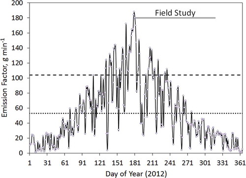Emission factors tended to be lowest in winter and autumn—coinciding with higher –and highest in summer when moisture content was lowest. The AP-42 value for E_v is plotted for comparison. A value of 104 g min⁻¹ (229 lb min⁻¹) was computed for the coal pile activity at the study site. Moisture content is not a factor in the AP-42-derived E_v so no daily variations exist. However, AP-42 allows assuming = 0 on days when precipitation ≥0.01 inches is observed. On many of those days, our moisture-sensitive E_v produces such low emissions that they are essentially zero anyway. The AP-42 E_v is twice the annual average E_v (53 g min⁻¹) derived from field data. In itself this difference is not too remarkable, given the uncertainty in the E_v estimates. What makes the AP-42 formulation inadequate is its inability to account for the effect of coal moisture on E_v, and this can produce large annual overestimates of fugitive emissions in regions where precipitation is plentiful for at least a portion of the year. Also, in situations where air quality modeling of fugitive emissions is required, a method for computing variations in E_v should produce more realistic results than assuming constant E_v.

Figure 7. Daily average coal moisture content for 2012 computed from hourly meteorological data measured near Nashville, TN, and eq 22. The period of the field study is denoted by the solid horizontal line in the upper part of the graph.

Figure 8. Daily emission factors for fugitive PM₁₀ coal dust calculated using the formulations for E_v versus M_c (eqs 23 and 24) and M_c plotted in Figure 7. The period of the field study is denoted by the solid horizontal line in the upper part of the graph. The E_v(AP) (= VE_ir) is represented by the horizontal dashed line near 100 g min⁻¹, and the annual average of E_v based on the study formulation is represented by the dashed line parallel to and below the line for E_v(AP).

E_v Sensitivity

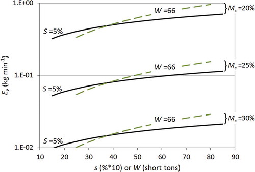
Although these results are specific to PRB coal, there is some question as to how to apply the derived EF formulation to other sites. First, note that vehicle speed is currently not a parameter used to estimate E_ir using the AP-42 formulation (eq 1) and may not vary sufficiently to enable quantification for work on a coal pile. Given that our E_v formulation produces values that are greater than, equivalent to, and less than those from AP-42 (i.e., E_v(AP)) depending on M_c, it is not unreasonable to assume that the two EF approaches provide insight into a common phenomenon that has been measured using two different methods. This is likely true within the accuracy of either methodology for determining E. Therefore, it is appropriate to combine the E_v formulation derived here with the sensitivity of E_ir to vehicle weight W and surface silt content s because the data on which E_v is based represent values of W and s that were within the range of values tested to develop the AP-42 E_ir formulation. Put another way, how could assuming similar sensitivities to W and s result in greater uncertainty than using a formulation not based on PRB coal that ignores M_c?

Let E_ir = f(s,W) represent eq 1. Assuming it is better to consider M_c than to apply a formulation that ignores it, it is suggested that

(26)

From this, it follows that

(27)

Equation 27 provides a means of computing E_v as a function of M_c, s, and W. The prime notation denotes new values of each variable derived from the values applicable in the present study (i.e., W° = 66 short tons, s° = 5%) and E_v° computed using eq 23, 24, or 25. This method of estimating E_v′ would not be advised for values of W′ and s′ outside the range of values that were associated with the studies on which eq 1 is based. The reader is referred to AP-42 for guidance. Although E_v sensitivity is somewhat greater to changes in s than W, coal silt content tends to vary less than vehicle weight from one situation to the next so that the latter is more likely to be important in individual situations. Figure 9 illustrates E_v response to the independent variables in eq 27. Emission factor sensitivity is largest in response to coal moisture, varying by nearly 2 orders of magnitude for in the range 20–30%. This E_v response is expected, given that water spraying is a standard technique for controlling fugitive dust emissions from aggregate material surfaces. The solid lines in Figure 9 denote E_v sensitivity to W with s = 5%. Dashed lines indicate E_v sensitivity to s with W = 66 short tons. Sensitivity to surface silt content is somewhat greater than to vehicle weight.

Figure 9. Sensitivity of E_v to various independent variables as determined from eq 27.

Conclusion

This study quantified the primary source of fugitive dust emissions from human activity on a PRB coal pile. Emissions from bulldozers working on the pile were estimated after removing the contribution from natural dust emissions. Bulldozer activity is needed to either groom or scrape the coal to minimize dust combustion or push coal around the pile (either toward an underground bunker for reclamation to the plant or to redistribute coal dumped onto the pile by the conveyor system). Coal dumping—another source of fugitive dust—occurred too infrequently to quantify its impact on dust levels.

It appears that downwind fugitive dust levels (as PM₁₀) from natural processes can occasionally be as high as or higher than levels from human activity. This makes it imperative that natural impacts on downwind concentrations be considered when using monitored concentrations to estimate fugitive dust impacts from human activity. Natural and human-made fugitive dust emissions produce similar downwind impacts, in part because both processes tend to remove similar-size particles by mechanical means from the same surface. Also, the lengths of time involved in natural and anthropogenic particle-emitting actions are similar in that both are transient processes that do not stay in one location for very long. Thus, both types of dust-emitting events share similar origins and similar downwind signatures.

The movement of bulldozers across the coal pile was associated with an increase in downwind concentrations of PM₁₀. Emissions of PM_2.5 were ≤6% of PM₁₀ emissions. Dispersion modeling of dust transported from the pile coupled with estimated anthropogenic levels of PM₁₀ derived EFs that were smaller than those computed using an AP-42 formulation, which was not developed using coal pile data and does not consider moisture effects. Uncertainty in the EFs was large because of the uncertainty in estimated levels of natural particles. However, daily averaging of EFs and coal moisture content revealed that the latter is an important predictor of emissions. In fact, the data indicate that the EF for fugitive coal dust decreases by two orders of magnitude as coal moisture content increases from 21 to 33% and essentially vanishes for M_c >33%. This is a valuable finding because the applicable AP-42 formulation does not allow for variation with coal moisture content.

Daily average coal moisture content was found to be strongly associated with precipitation, air temperature, and solar radiation, parameters that serve as surrogates for water input and evaporation processes. Time-lagged surface moisture is an even better predictor of daily surface moisture because it provides a superior representation of time-integrated factors controlling the surface water balance (i.e., it eliminates the need for temperature or rainfall history in the form of previous-day temperature and precipitation data). A time series of surface moisture can be built from available data on precipitation and solar radiation. Potential meteorological predictors are available from on line National Oceanic and Atmospheric Administration (NOAA) data records and can be used to estimate fugitive coal dust emissions for periods when it is not raining and temperatures average above freezing. An alternate estimation methodology would be needed for wintertime in cold climates. The value of this approach is evident for plants located where frequent rainfall tends to add moisture to the coal, with the resulting emissions being lower than those otherwise derived using AP-42.

All of the preceding conclusions are for a PRB coal pile. The characteristics of PRB coal (average silt content of 5%) are such that the EFs derived in this study may overstate emissions from work on piles composed of different coal types. However, the moisture effect may also be unique to PRB coal. Additional research is needed to determine whether the EFs derived here are applicable to other coals.

Funding

The authors are grateful to the Gallatin plant personnel who supported the field measurement phase of this effort. Funding for this work was provided by the Electric Power Research Institute and the Tennessee Valley Authority.

Additional information

Notes on contributors

Stephen F. Mueller

Stephen F. Mueller, Jonathan W. Mallard, and Qi Mao perform environmental studies for the Tennessee Valley Authority.

Jonathan W. Mallard

Stephen F. Mueller, Jonathan W. Mallard, and Qi Mao perform environmental studies for the Tennessee Valley Authority.

Qi Mao

Stephen F. Mueller, Jonathan W. Mallard, and Qi Mao perform environmental studies for the Tennessee Valley Authority.

Stephanie L. Shaw

Stephanie L. Shaw is a senior project manager for air quality studies at Electric Power Research Institute.

References

- Cowherd, C., Jr., K. Axetell, Jr., C.M. Guenther, and G.A. Jutze. 1974. Development of Emission Factors for Fugitive Dust Sources, Midwest Research Institute report to the EPA. EPA-450/3-74-037. http://nepis.epa.gov/Adobe/PDF/2000MC6B.PDF.
- Ghose, M.K. 2004. Emission factors for the quantification of dust in Indian coal mines. J. Sci. & Ind. Res. 63, 763–768.
- Mueller, S.F., J.W. Mallard, Q. Mao, and S.L. Shaw, 2013. Fugitive particulate emission factors for dry fly ash disposal. J. Air Waste Manage. Assoc. 63. doi:10.1080/10962247.2013.795201
- Mueller, S.F., J.W. Mallard, and S.L. Shaw. 2015. Variability of natural dust erosion from a coal pile. J. Appl. Meteor. Climatol. doi:10.1175/JAMC-D-14-0126.1
- U.S. Environmental Protection Agency. 1995 with subsequent updates. Compilation of Air Pollutant Emission Factors—Volume I: Stationary Point and Area Sources, AP-42 Fifth Edition. Research Triangle Park, NC: Office of Air Quality Planning and Standards.
- U.S Environmental Protection Agency. 1998. Revision of emission factors for AP-42 Section 11.9—Western Surface Coal Mining. Prepared by the Midwest Research Institute for Office of Air Quality Planning and Standards. Research Triangle Park, NC. http://pubs.usgs.gov/pp
- U.S. Environmental Protection Agency. 2004. User’s Guide for the AMS/EPA Regulatory Model—AERMOD. EPA-454/B-03-001. Research Triangle Park, NC: Office of Air Quality Planning and Standards.
- U.S. Geological Survey. 1999. Coal quality and geochemistry, Powder River Basin, Wyoming and Montana. In 1999 Resource Assessment of Selected Tertiary Coal Beds and Zones in the Northern Rocky Mountains and Great Plains Region, chapter PQ. Report 1625-A, p. 27. http://pubs.usgs.gov/pp/p1625a/Chapters/PQ.pdf
- Venkatram, A. 2000. A critique of empirical emission factor models: A case study of the AP-42 model for estimating PM10 emissions from paved roads. Atmos. Environ. 34:1–11. doi:10.1016/S1352-2310(99)00330-1
- Venkatram, A., D. Fitz, K. Bumiller, S. Du, M. Boeck, and C. Ganguly, 1999. Using a dispersion model to estimate emission rates of particulate matter from paved roads. Atmos. Environ. 33:1093–1102. doi:10.1016/S1352-2310(98)00316-1
- Western Regional Air Partnership. 2005. Analysis of the fine fraction of particulate matter in fugitive dust—Final report, Midwest Research Institute report for the Western Governors’ Association Western Regional Air Partnership. http://www.epa.gov/ttnchie1/ap42/ch13/related/mri_final_fine_fraction_dust_report.pdf.