The geographic distribution and economic value of climate change-related ozone health impacts in the United States in 2030

Abstract

In this United States-focused analysis we use outputs from two general circulation models (GCMs) driven by different greenhouse gas forcing scenarios as inputs to regional climate and chemical transport models to investigate potential changes in near-term U.S. air quality due to climate change. We conduct multiyear simulations to account for interannual variability and characterize the near-term influence of a changing climate on tropospheric ozone-related health impacts near the year 2030, which is a policy-relevant time frame that is subject to fewer uncertainties than other approaches employed in the literature. We adopt a 2030 emissions inventory that accounts for fully implementing anthropogenic emissions controls required by federal, state, and/or local policies, which is projected to strongly influence future ozone levels. We quantify a comprehensive suite of ozone-related mortality and morbidity impacts including emergency department visits, hospital admissions, acute respiratory symptoms, and lost school days, and estimate the economic value of these impacts. Both GCMs project average daily maximum temperature to increase by 1–4°C and 1–5 ppb increases in daily 8-hr maximum ozone at 2030, though each climate scenario produces ozone levels that vary greatly over space and time. We estimate tens to thousands of additional ozone-related premature deaths and illnesses per year for these two scenarios and calculate an economic burden of these health outcomes of hundreds of millions to tens of billions of U.S. dollars (2010$).

Implications: Near-term changes to the climate have the potential to greatly affect ground-level ozone. Using a 2030 emission inventory with regional climate fields downscaled from two general circulation models, we project mean temperature increases of 1 to 4°C and climate-driven mean daily 8-hr maximum ozone increases of 1–5 ppb, though each climate scenario produces ozone levels that vary significantly over space and time. These increased ozone levels are estimated to result in tens to thousands of ozone-related premature deaths and illnesses per year and an economic burden of hundreds of millions to tens of billions of U.S. dollars (2010$).

Introduction

Climate change can affect air pollutant concentrations in a myriad of ways. Meteorological factors, such as temperatures, cloudiness, precipitation frequency and intensity, wind speeds, and planetary boundary layer heights, are all first-order drivers that influence air quality by determining photochemical reaction rates, vertical mixing, horizontal transport, biogenic emissions, and rates of pollutant removal by wet and dry deposition. Over longer time scales, climate change may also affect land use and population density, modifying emissions and meteorology and thus further affecting air quality. That these factors are related through a number of complex nonlinear pathways makes it challenging to model the individual role of each variable in a comprehensive framework.

For example, many epidemiological studies and risk assessments that examined the influence of climate change on air quality held most factors constant and allowed only a limited number of input parameters to vary (Tagaris et al., 2009; Selin et al., 2009; Bell et al., 2007; Jacobson, 2008; Silva et al., 2013; Post et al., 2012). Bell et al. (2007) project ozone levels to the year 2050 in 50 eastern U.S. cities using the Intergovernmental Panel on Climate Change (IPCC) Fourth Assessment Report A2 emission scenario and describe how climate change increases ozone-related daily mortality by maintaining constant anthropogenic emissions and allowing meteorology to vary over time. That study attempted to isolate the role of climate change on future meteorology and its subsequent effect on human health, holding all other factors constant. Other assessments quantify the effects of historical changes in climate, making it challenging to identify the factor(s) most responsible for climate-related effects. For example, Jacobson (2008) relates historical changes in CO₂ levels to ambient ozone concentrations and the risk of premature death. Silva et al. (2013) quantifies the human health burden due to total anthropogenic outdoor air pollution and further characterizes the portion of this burden attributable to past climate change.

Climate and air quality modeling are each time and resource intensive, so simulations focus on a limited number of projected years, climate scenarios, and geographic locations (Chang, Zhou, and Fuentes, 2010; Sheffield et al., 2011; Chang, Hao, and Sarnat, 2014; Jackson et al., 2010). Sheffield et al. (2011) relate asthma emergency department visits in the 2020s in the New York City metropolitan area to simulated ozone changes using the IPCC A2 emission scenario. Chang et al. (2014) use a series of general circulation models (GCMs) and regional climate models to estimate the change in ozone-related emergency department visits due to climate change in the Atlanta, GA, metropolitan area.

Taken together, these time, resource and data constraints pose special challenges to disentangling the influence of each factor that might affect climate, air quality, and health. For this reason, analyses of relationships between air quality, climate and health generally alter a subset of input parameters such as the climate model or assumptions regarding future growth in emissions, or limit the geographical extent of the modeled air quality domain. Because calculating health impacts is comparatively computationally efficient, it is relatively easy to test the sensitivity of the results to various input parameters.

We select among the existing suite of climate models, greenhouse gas forcing scenarios, and population projections to examine the scope, magnitude, spatial distribution and economic value of climate-change related air quality and health impacts in the year 2030 relative to meteorology in the year 2000. Specifically, in this analysis we use multiple years within a time slice centered on 2030 from two GCMs and different climate forcing scenarios to account for different assumptions regarding the influence of future greenhouse gas concentrations on climate and to account for year-to-year variability in projected air quality impacts. We characterize the near-term influence of a changing climate on tropospheric ozone-related health impacts near the year 2030, which is a policy-relevant time frame that is subject to fewer uncertainties than previous studies that have focused on 2050 or later (e.g., Post et al., 2012).

In this study, we account for federal air quality policies requiring that areas meet the health-based National Ambient Air Quality Standard (NAAQS) for ozone. Our modeling reflects the emissions controls that have been adopted to reduce anthropogenic emissions of nitrogen oxides (NOx) and volatile organic compounds (VOCs), which will decline significantly between the present day and 2030. Our research aim is not to predict future ozone levels, but rather to quantify and monetize the “climate penalty” (Wu et al., 2008). That is, we seek to estimate the influence of near-term climate change on ozone, and the resulting health impacts and economic burden of those health impacts. We use the same anthropogenic emissions for the historical (ca. 2000) and future (ca. 2030) air quality modeling to isolate the influence of climate change on air quality, employing a 2030 emissions inventory that accounts for fully implementing existing anthropogenic emissions controls, which will strongly influence future tropospheric ozone levels. We quantify a comprehensive suite of ozone-related mortality and morbidity impacts including emergency department visits, hospital admissions, acute respiratory symptoms, and lost school days and estimate the economic value of these impacts. This analytical approach yields estimated climate change-attributable ozone-related premature deaths and illnesses that better account for the baseline atmospheric environment that is expected to prevail in the United States at 2030, as well as differences in climate scenarios and variability in predicted ozone levels across years and locations.

In the following, we first describe the methods we employ to project ozone levels and human health impacts. Next, for each scenario we report the ozone-related health impacts and the economic value of these outcomes; then we discuss the implications of these results.

Methods

Here we apply a suite of modeling tools that are linked sequentially to quantify (a) global climate impacts from specified greenhouse gas forcing scenarios, (b) the resultant regional climate changes over the United States at a higher spatial resolution, (c) the resultant near-surface ozone impacts over the United States driven by the regional climate, and (d) the resultant health impacts and economic value in the United States of climate-related changes in 2030 ozone air pollution levels (Figure 1).

Figure 1. Overview of analytical approach to estimating climate-related ozone changes, health impacts, and economic values.

Regional climate modeling

We used fields from two different GCMs that participated in the fifth phase of the Coupled Model Intercomparison Project (CMIP5) (Taylor, Stouffer, and Meehl, 2012). For each GCM, we downscaled two 11-year time slices: the 1995–2005 period from the historical 20th-century experiment, and the period 2025–2035 following one of the Representative Concentration Pathways (RCPs) (van Vuuren et al., 2011):

1. RCP 8.5 modeled with the National Center for Atmospheric Research/Department of Energy (NCAR/DOE) Community Earth System Model (CESM) (hereafter referred to as “CESM/RCP 8.5”).

2. RCP 6.0 modeled with the NASA Goddard Institute for Space Studies (GISS) Model E2 (hereafter referred to as “GISS/RCP 6.0”).

The RCP 8.5 scenario (Riahi et al., 2011) assumes “business as usual,” where greenhouse gases will increase substantially over the next century, eventually leading to an 8.5 W m⁻² radiative forcing level by 2100. The RCP 6.0 scenario (Fujino et al., 2006) assumes a modest degree of mitigation of greenhouse gas emissions such that total radiative forcing will increase over the next century before stabilizing at 6.0 W m⁻² in 2100.

We downscaled these GCM projections using the Weather Research and Forecasting (WRF) model following techniques described by Bowden et al. (2012) and Otte et al. (2012). We conducted WRF simulations at 36-km horizontal grid spacing over the United States, incorporating the global climate forcing at the lateral boundaries, through the interior of the domain (following Otte et al., 2012), and in the sea-surface temperatures. It is important to recognize that climate simulated by and downscaled from GCMs for a particular historical (or future) day cannot be compared directly with the actual meteorology that occurred (or will occur) on that day. Rather, the historical period 1995–2005 is intended to be representative of the year 2000, while the future period (2025–2035) is intended to be representative of 2030.

Air quality modeling

The historical and future climate WRF outputs were processed by the Meteorology–Chemistry Interface Processor (MCIP) (Otte and Pleim, 2010) and subsequently input into the Community Multi-scale Air Quality model (CMAQ) version 5.0.1 (Byun and Schere, 2006) to assess how the climate-driven meteorological changes would impact near-surface ozone levels (i.e., concentrations within the lowest model layer, about 38 m deep) over the continental United States. The air quality modeling was also conducted at 36-km grid spacing. While 36-km regional climate and air quality modeling would not be appropriate for projecting future ozone values in individual locations, this resolution is suitable for assessing the sensitivity of future regional-scale ozone levels to climate-driven changes in meteorology. The chemical lateral boundary conditions in the air quality modeling are based on an independent simulation of the year 2011 using the GEOS-Chem global chemical transport model (Bey et al., 2001). The time-varying chemical boundary conditions are used for each year and are unchanged between the base and future climate case. Thus, any changes in ozone transported into the domain are not assessed in this analysis.

For the CESM/RCP 8.5 scenario we used CMAQ to simulate each of the 11 historical years (1995–2005) and 11 future years (2025–2035) to capture the impacts of potential inter-annual variability in the climate response. For the GISS/RCP 6.0 scenario, we identified three historical and three future years that were least conducive, moderately conducive, and most conducive to forming near-surface ozone across the entire continental United States. These years were identified using previous CMAQ simulations of the same 11-year periods that had been forced with present-day emissions, but were otherwise identical to the configuration applied here. The annual number of exceedances of 75 ppb for daily maximum 8-hr ozone were tallied within model grid cells throughout the United States; then the years of each 11-year simulation period were ranked. The most (least) conducive year contained the most (least) exceedances of the threshold, and the moderately conducive year was the median year of each 11-year simulation period. Due to the computational costs associated with air quality modeling, only the regional climate fields from these two 3-year subsets of the GISS/RCP 6.0 were combined with the 2030 emissions in the CMAQ simulations used in the present study.

In this study, only the meteorological conditions (and specific emissions sectors that depend upon meteorology) were changed within the historical and future CMAQ runs to isolate the climate impacts in each scenario—all other input variables were held constant in the air quality modeling scenarios. The emissions were based on U.S. Environmental Protection Agency (EPA) estimates of 2030 levels, which assume the implementation of air quality policies affecting ozone precursor emissions such as the Mercury and Air Toxics Standards and the Tier-2 rule affecting mobile sources (EPA, 2011a,b; EPA, 2012). Biogenic and sea salt emissions were allowed to vary according to climate-driven meteorological changes, but emissions from mobile sources, electrical generating units, and wildfires did not change as a function of climate.

Estimating health impacts

We assess health impacts associated with surface-level ozone in the 5969 36-km grid cells in the continental United States. In each grid cell, we apply a health impact function relating changes in ambient concentrations with ozone-related adverse outcomes. A log-linear health impact function, which we use to quantify most of the impacts in this analysis, is illustrated by eq 1:

(1)

where is the change in the incidence of a particular health endpoint attributable to the change in ozone concentration (∆X), Pop and Y₀ are the population and baseline incidence rates for the year 2030, and β is the concentration-response factor drawn from the epidemiology literature. We calculate impacts using the environmental Benefits Mapping and Analysis Program–Community Edition (BenMAP-CE), v1.08 (EPA, 2014), following EPA regulatory analyses and similar studies in the literature (Fann et al., 2011).

We estimated the change in ozone-related adverse human health outcomes of several health endpoints the U.S. Environmental Protection Agency (EPA) quantified in a recent regulatory impact analysis (EPA, 2010) for the Ozone NAAQS. The EPA quantified health outcomes that the EPA Integrated Science Assessment (ISA) determined were causally, or likely to be causally, related to ozone exposure (EPA, 2014). When selecting among epidemiological studies to use as the basis for constructing health impact functions, the agency considered an array of attributes, including statistical design (e.g., time series, case crossover, etc.); time period analyzed; population attributes; population size; and pollutant measures, among other characteristics. In brief, the agency selected studies for which the attributes made them most appropriate for an air pollution health impact analysis. A complete description of the systematic approach to selecting studies can be found in the Regulatory Impact Analysis for the Particulate Matter NAAQS (EPA, 2012). Consistent with the guidance provided by the National Academies of Sciences, and as a means of characterizing uncertainty in the ozone-mortality relationship, we report premature deaths attributable to short-term (i.e., day-to-day) changes in ozone using effect estimates from a suite of multicity studies and meta-analyses (National Research Council, 2008).

For both the GISS/RCP 6.0 and CESM/RCP 8.5 scenarios we estimate air pollution-related health impacts at 2030 using Integrated Climate and Land Use Scenarios (ICLUS) population projections (EPA, 2009; Bierwagen et al., 2010). ICLUS projects the county-level population distribution using assumptions consistent with the IPCC Special Report on Emission Scenarios (SRES) (IPCC, 2000). For this analysis we selected ICLUS projections for SRES A1 and B2, which are roughly consistent with RCP 8.5 and RCP 6.0, respectively. In a sensitivity analysis, we also examine the impact of using ICLUS A1 and B2 population projections to 2050, as well as another population projection developed for 2030 (Woods and Poole, 2012) (Supplemental Figure 1).

We estimate ozone-related effects on premature death, emergency department visits for asthma, hospital visits for respiratory causes, acute respiratory symptoms, and lost school days. We calculate ozone-related premature deaths using cause-specific mortality rates (referenced as Y₀ in the preceding equation) provided by the Centers for Disease Control and Prevention (CDC, 2008) that we projected to the year 2030 using information provided by the U.S. Census Bureau; these projected mortality rates do not account directly for the influence of climate or air quality changes. Morbidity rates are more difficult to project in the future, and we use cause-specific morbidity rates for the year 2007, assuming constant rates over time, though they are likely to change in reality (Tables 1 and 2 of Supplemental Material). We use the seasonal (May–September) average of the 8-hr daily maximum (MDA8) ozone concentration in each 36-km grid cell from CMAQ. Gridded health impact results are aggregated according to six climate regions used by the National Climate Assessment (NCA) in Supplemental Figure 1 (National Climate Assessment, 2014).

Estimating the economic value of health impacts

To estimate the economic value of the health impacts of a changing climate on air quality, we assign a dollar value to the incidence of premature deaths and illnesses occurring in 2030. We derive both cost of illness (COI) and willingness to pay (WTP) measures from the published economic literature, which we then multiply by the counts of adverse health outcomes to express the economic value of these impacts. COI metrics generally account for the value of medical expenditures to treat the adverse outcome and sometimes also the value of the productivity lost due to the illness (e.g., time spent in the hospital). By contrast, WTP measures are generally understood to account for the value that individuals place on both these direct costs as well as the value they place on avoiding pain and suffering (Harrington and Portney, 1987; Berger and Blomquist, 1987). For this reason, economic benefit analyses of air pollution impacts tend to prefer WTP values when they are available.

As in the preceding, we use economic value estimates that are consistent with recent EPA Regulatory Impact Analyses. We estimate the value of statistical life (VSL) to characterize the economic value of ozone-related premature deaths. VSL is a summary measure that expresses the economic value of small changes in the risk of premature death to a large number of people, and is not intended to describe the economic value of any particular life. In this analysis we use a EPA Science Advisory Board-recommended VSL that is derived from a meta-analysis of 26 individual studies (EPA Health Effects Subcommittee, 2010). Because the willingness to pay to reduce mortality and morbidity risk will grow with personal income, and in this analysis we quantify values in a future year, we adjusted each WTP measure; for VSL this value is $9.9 million in 2030 (2010 dollars). We value health outcomes including respiratory hospital admissions, emergency department visits, and lost school days using COI measures and value acute respiratory symptoms using a WTP measure. The source of this literature and the unit values are summarized in Supplemental Table 3.

Results

We first report the ozone-related impacts and dollar values for each of the two climate scenarios that have been calculated using projected ozone levels averaged across the scenario years. Next we characterize the spatial distribution of these impacts by NCA region and the interannual variability.

Air quality changes

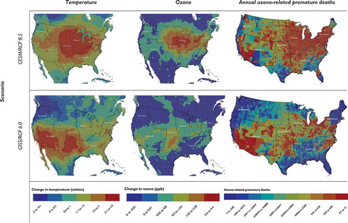
Both the CESM/RCP 8.5 and GISS/RCP 6.0 scenarios are associated with large changes in daily maximum temperatures over the months when ozone levels tend to be highest over the United States. In both scenarios, average daily maximum temperatures are projected to increase by 1–4°C over a broad swath of the continental U.S. (Figure 2). The locations of the largest projected temperature increases vary by scenario, and the average U.S. warming is greater in the CESM/RCP 8.5 scenario, as could be expected. Concurrently, other pollution-relevant weather variables (not shown) are also projected to change. The net effect on near-surface ozone is shown in Figure 2. Seasonal (May–September) mean increases in MDA8 ozone levels of 1–5 ppb are common in the CESM/RCP 8.5 scenario, resulting in more exceedances of the 75-ppb ozone NAAQS than in the historical climate case. The GISS/RCP 6.0 scenario also shows large increases in ozone over some parts of the country (e.g., central United States, California) but projects decreases in ozone over other locations (e.g., Pacific Northwest, Gulf Coast).

Figure 2. Projected change in average daily maximum temperature, seasonal average maximum daily 8-hr ozone, and ozone-related premature deaths in 2030.

Average health impact estimates and economic values in 2030

As a means of describing a central tendency estimate of ozone-related health impacts in the year 2030, we report first the number of premature deaths and illnesses calculated from the average projected ozone values for the 3 individual year GISS/RCP 6.0 and 11 sequential year CESM/RCP 8.5 climate scenarios. We estimate a greater overall number of premature deaths and illnesses for the CESM/RCP 8.5 scenario than the GISS/RCP 6.0 scenario. As shown in Table 1, using GISS/RCP 6.0, we project tens to hundreds of premature deaths, hundreds of respiratory emergency department and hospital visits, tens of thousands of days of missed school, and hundreds of thousands of cases of acute respiratory symptoms. The impact is one order of magnitude greater in each category using CESM/RCP 8.5, as we project hundreds to thousands of premature deaths, thousands of respiratory emergency department and hospital visits, hundreds of thousands of days of missed school, and more than 1 million cases of acute respiratory symptoms.

Table 1. Additional ozone-related premature deaths and illnesses attributable to climate change in 2030 in the continental United States (95% confidence intervals)

Health outcome^a	Climate scenario^b
	GISS/RCP 6.0	CESM/RCP 8.5
Alternative estimates of ozone-related premature death (ages 0–99 years)
Bell et al. (2004)	37	420
	(12–61)	(140–700)
Huang, Dominici, and Bell (2004)	56	640
	(21–92)	(240–1000)
Schwartz (2005)	56	640
	(17–94)	(200–1100)
Bell, Dominici, and Samet (2005)	120	1300
	(56–180)	(630–2000)
Ito, De Leon, and Lippmann (2005)	160	1900
	(98–230)	(1100–2600)
Levy, Chemerynski, and Sarnat (2005)	170	1900
	(110–220)	(1300–2500)
Respiratory hospital admissions (ages 0–1 and 65–99 years)	360	3900
	(65–870)	(1600–8000)
Respiratory emergency department visits (ages 0–99 years)	89	1200
	(82–310)	(1000–4300)
Acute respiratory symptoms (ages 18–64 years)	210,000	1,900,000
	(86,000–330,000)	(780,000–3,000,000)
Missed days of school (ages 5–17 years)	67,000	650,000
	(23,000–150,000)	(230,000–1,500,000)

Notes: ^aEstimates rounded to two significant figures.

^bThe 2030 ozone levels calculated by averaging each modeled year of ozone levels—three selected years for GISS/RCP 6.0 and 2025–2035 for CESM/RCP 8.5.

The estimated economic value of these premature deaths and illnesses is substantial (Table 2). We estimate the value of the hospital admissions, emergency department visits, missed days of school, and acute respiratory symptoms for the GISS/RCP 6.0 scenario in the tens of millions of U.S. dollars, and hundreds of millions of dollars for the CESM/RCP 8.5 scenario (2010 dollars). We estimate the value of the additional premature deaths to be in the hundreds of millions of dollars for the GISS/RCP 6.0 scenario, and in the tens of billions of dollars for the CESM/RCP 8.5 scenario. To characterize the total dollar value of the additional premature deaths and illnesses, we report the sum of these impacts, finding that the economic value of these adverse outcomes ranges from $320 million to $1.4 billion for the GISS/RCP 6.0 scenario and from $3.6 to $15 billion for the CESM/RCP 8.5 scenario.

Table 2. Economic value of ozone-related premature deaths and illnesses attributable to climate change in 2030 (95% confidence intervals, millions of 2010 dollars)

Health outcome^a	Climate scenario^b
	GISS/RCP 6.0	CESM/RCP 8.5
Alternative estimates of ozone-related premature death (ages 0–99 years)
Bell et al. (2004)	$290	$3400
	($24–$870)	($280–$10,000)
Huang, Dominici, and Bell (2004)	$450	$5200
	($38–$1300)	($430–$15,000)
Schwartz (2005)	$450	$5100
	($36–$1300)	($410–$15,000)
Bell, Dominici, and Samet (2005)	$940	$11,000
	($82–$2700)	($940–$31,000)
Ito, De Leon, and Lippmann (2005)	$1300	$15,000
	($120–$3700)	($1400–$42,000)
Levy, Chemerynski, and Sarnat (2005)	$1300	$15,000
	($120–3600)	($1400–$41,000)
Respiratory hospital admissions (ages 0–1 and 65–99 years)	$11	$100
	($2–$19)	($10–$130)
Respiratory emergency department visits (ages 0–99 years)	$0.04	$0.5
	($0.01–$0.1)	($0.3–$1.3)
Acute respiratory symptoms (ages 18–64 years)	$13	$120
	($5–$25)	($45–$220)
Missed days of school (ages 5–17 years)	$7	$64
	($3–$9.4)	($28–$91)
Total economic value of ozone-related premature deaths and illnesses
Sum of Bell et al. 2004 and each morbidity outcome	$320	$3600
	($34–$920)	($350–$10,000)
Sum of Levy et al. 2005 and each morbidity outcome	$1400	$15,000
	($130–$3700)	($1500–$41,000)

Notes: ^aEstimates rounded to two significant figures.

^bThe 2030 ozone levels calculated by averaging each modeled year of ozone levels—three selected years for GISS/RCP 6.0 and 2025–2035 for CESM/RCP 8.5.

Health impacts by geographic region

In the figures described next, we describe how the ozone-related premature deaths are distributed throughout the United States for each climate scenario. Figure 2 plots the distribution of temperature and ozone (at 36-km grid cells) and climate change-attributable premature deaths (at each county), illustrating the relationship between these three variables. The GISS/RCP 6.0 scenario projects the greatest increases in temperature in the southwestern United States, where CMAQ consequently projects increases in ozone levels. Likewise, we estimate the greatest number of ozone-related deaths to occur in metropolitan areas affected by this temperature change, including Los Angeles, CA, and Dallas, TX. Separately, the CESM/RCP 8.5 scenario projects higher temperatures and ozone levels in the midwestern United States. Under this scenario, we project cities including Chicago, IL, and New York, NY, to see an increase in the number of ozone-related premature deaths.

Interannual variability

The aggregated results already reported do not reflect the substantial year-to-year variability in simulated temperature and ozone changes. Here we examine the influence of meteorological interannual variability on ozone levels and resulting estimated health impacts. We compare several individual future year simulations against the 3-year GISS/RCP 6.0 and 11-year CESM/RCP 8.5 scenario averages of the present-day years to better understand how future inter-annual variability can affect results. We select three future years for each of the two climate models that represent the least conducive, moderately conducive, and most conducive years for forming ozone levels above the current NAAQS for ozone (75 ppb) and predict ozone-related premature deaths in each of those three years using an array of short-term ozone mortality risk coefficients (Table 3). Those years with meteorology projected to be least and moderately conducive to forming ozone in the GISS/RCP 6.0 scenario yield a net reduction in ozone-related deaths and illnesses as compared to a baseline that does not reflect climate change. In the year most conducive to forming ozone in the GISS/RCP 6.0 scenario, we predict a net increase in the number of ozone-related premature deaths. By contrast, the year that is predicted to be least conducive to forming ozone in the CESM/RCP 8.5 scenario yields a net reduction in ozone-related deaths and illnesses, while the moderately and most conducive years yield substantial increases in ozone health impacts.

Table 3. Estimated number of additional ozone-related premature deaths and illnesses attributable to projected change in the U.S. climate (95% confidence intervals)

	GISS/RCP 6.0			CESM/RCP 8.5
	Years least, moderately, and most conducive to forming ozone			Years least, moderately, and most conducive to forming ozone
Health outcome^a	Least (2035)	Moderately (2027)	Most (2025)	Least (2028)	Moderately (2030)	Most (2035)
Alternative estimates of ozone–related premature death (ages 0–99 years)
Bell et al. (2004)	–220	–6	340	–32	400	870
	(–75 to –380)	(–2 to –9)	(110 to –570)	(–11 to –53)	(230–670)	(290–1500)
Huang, Dominici, and Bell (2004)	–350	3	520	–48	620	1,300
	(–130 to –570)	(1–4)	(190–840)	(–18 to –77)	(230–1000)	(500–2200)
Schwartz (2005)	–340	–8	520	–49	620	1300
	(–100 to –580)	(–3 to –14)	(160–880)	(–15 to –83)	(190–1000)	(410–2600)
Bell, Dominici, and Samet (2005)	–720	–21	1,100	–110	1300	2800
	(–340 to –1,100)	(–10 to –38)	(520–1,700)	(–53 to –170)	(610–2000)	(1300–4300)
Ito, De Leon, and Lippmann (2005)	–1000	–25	1500	–140	1800	3900
	(–600 to –1400)	(–15 to –34)	(920–2100)	(–87 to –200)	(1100–2500)	(2400–5500)
Levy, Chemerynski, and Sarnat (2005)	–1000	–29	1500	–160	1800	3900
	(690 to –1300)	(–20 to –38)	(1100–2000)	(–110 to –210)	(1200–2400)	(2700–5200)
Respiratory hospital admissions (ages 0–1 and 65–99 years)	–1900	–130	3,100	–250	3500	7500
	(–280 to –4100)	(–42 to –260)	(6800–1100)	(–110 to –560)	(2200–5700)	(5000–12,000)
Respiratory emergency department visits (ages 0–99 years)	–510	–3	770	38	1200	2500
	(–420 to –1700)	(–14 to –4)	(–720 to 2700)	(17—86)	(530–2600)	(1100–5600)
Acute respiratory symptoms (ages 18–64 years)	–950,000	–2400	1,600,000	–180,000	1,900,000	4,000,000
	(–390,000 to –1,500,000)	(–380 to –6100)	(650,000–2,500,000)	(75,000–280,000)	(780,000–3,000,000)	(1,600,000–6,300,000)
Missed days of school (ages 5–17 years)	–310,000	–4,000	500,000	–81,000	660,000	1,400,000
	(–110,00 to –670,000)	(–6300 to –1500)	(180,000–1,100,000)	(28,000–110,000)	(600,000–730,000)	(1,300,000–1,500,000)

Note: ^aEstimates rounded to two significant figures.

All 11 projected years of ozone changes under the CESM/RCP 8.5 scenario were used to examine the annual variability in ozone-related premature deaths within the 6 NCA climate regions (Figure 3). The Northwest, the Great Plains, and the Southwest regions are projected to incur few ozone related health impacts, while the Northeast and Midwest regions are projected to have increases in ozone-related deaths (i.e., reductions in mortality avoided) for most of the years.

Figure 3. Annual number of climate-attributable ozone-related premature deaths by region and year for the CESM/RCP 8.5 scenario.

Discussion

For the two climate scenarios in which we modeled ozone-related air quality changes in 2030, we estimate hundreds to thousands of premature deaths, hundreds to thousands of respiratory emergency department and hospital visits, tens of thousands to hundreds of thousands of days of missed school, and hundreds of thousands to millions of cases of acute respiratory symptoms. We find that the economic value of these impacts is in the hundreds of millions to billions of dollars. These estimates vary greatly according to the combined climate model and RCP simulated, as we estimate much greater impacts using the CESM/RCP 8.5 scenario than we do with the GISS/RCP 6.0 scenario. Likewise, we find that the scope and magnitude of these impacts vary significantly across the scenarios and between individual years. The CESM/RCP 8.5 scenario generally predicts greater ozone formation in the Midwest, while we estimate higher ozone levels in the Southwest under the GISS/RCP 6.0 scenario. Consistent with previous health impact analyses that account for ozone-related effects, the impacts we report are also greatly influenced by the concentration-response relationship used to quantify the incidence of premature deaths.

This work is similar in some respects to studies published elsewhere in the literature. For example, Post et al. (2012) used an earlier version of the BenMAP tool to quantify climate-change-attributable national-level ozone-related premature death and illnesses and applied similar baseline incidence rates and concentration-response functions. However, that study used year 2050 ozone predictions from seven climate scenarios based on earlier generations of GCMs and did not characterize the economic value of those impacts. That paper reported climate-change-attributable ozone-related premature deaths that varied significantly across scenarios and approaches to projecting future population, and ranged from thousands of additional deaths to hundreds of avoided deaths.

Tagaris et al. (2009) quantified the sensitivity of ozone and fine particle levels in 2050 to marginal changes in precursor emissions including NOx, NH₃, and SO₂ and further quantified the number of premature deaths attributable to changes in these two pollutants. Because that paper reported changes in premature deaths as a function of marginal changes in ozone levels, it is difficult to compare those estimates to the results reported here. Bell et al. (2007), as described earlier, characterized ozone-related impacts in the year 2050 within 50 Eastern cities, holding anthropogenic emissions constant. None of the studies already described assign a dollar value to the avoided/incurred deaths and illnesses.

There are several unique facets to this study. First, we use GCM versions conducted for CMIP5 that include more than 10 years of further model developments beyond those used previously, as well as taking advantage of recent advances in regional climate modeling techniques. Second, we quantify effects in the year 2030 using an EPA emissions inventory that accounts for emission control measures expected to affect the level and distribution of ozone precursor emissions. Third, we characterize the variability in ozone-related impacts over both space (by U.S. county) and time (for each of the projected scenario years). Finally, we assign a dollar value to these projected ozone-related health impacts, giving insight to the potential economic value of this particular aspect of future climate change.

Limitations

As with any analysis of this scope and complexity, there are several notable limitations and uncertainties. First, we considered only two Representative Concentration Pathways (RCP 6.0 and RCP 8.5) that were modeled using two GCMs (GISS and CESM). Modeling each RCP using a different climate scenario means that differences in the predicted ozone levels and health impacts are attributable to both the RCP and the GCM.

Second, several emissions categories that are important to forming ozone, and could potentially be affected by climate (e.g., mobile sources, EGUs, and wildfires), are unchanged between the contemporary-climate and projected-climate air quality modeling. Other studies have shown linkages between a warmer climate and increased evaporative emissions from mobile sources (Rubin et al., 2006), increased electricity usage (Mideksa and Kallbekken, 2010), and increased wildfire activity over parts of the United States (Yue et al., 2013), all of which could lead to even greater health impacts from climate than shown here.

Third, using 36-km grid spacing (as was done here) does not consider potentially important interactions between meteorology, ozone, and health at the local scale, particularly within urban areas. However, adding higher spatial resolution to more finely resolve urban areas would add at least an order of magnitude more computational expense to this analysis. Fourth, we assume concentration-response relationships are constant over time, although changing populations, concentrations, baseline health status, and air pollution mixtures would almost certainly alter the relationship. Likewise, we assume baseline morbidity rates are constant over time, though they are likely to change as a result of changing economic and demographic conditions. Similarly, we did not account for the potential for climate-induced changes in temperature to increase (or decrease) ozone-related risks (Ren, Williams, and Tong, 2006; Ren, Williams, and Mengersen, 2009; Jhun et al., 2014). Fifth, because quantifying climate-induced PM_2.5 changes is even more strongly related to emissions changes that we did not model (e.g., wildfires), we did not include fine particle levels for this analysis. Many of these assumptions and limitations are consistent with other assessments of future climate-induced air quality changes in the literature (Post et al., 2012).

It is also important to note that this analysis does not account for policies that might mitigate the impacts estimated here, apart from those policies that are already expected to be in place by 2030. For example, while this modeling projects that climate change will create meteorological conditions more conducive to forming ozone, and hence increase the ground-level ozone in many parts of the country, we did not attempt to model air quality management adaptation scenarios that could reduce the level of ozone precursor emissions that would occur in response to these climate-driven impacts. To the extent that climate change increases ambient ozone concentrations (and/or other criteria pollutants) above the health-based air quality standards, the Clean Air Act directs states and municipalities to attain the standard by developing policies to reduce these ambient levels (Bachmann, 2007).

Conclusion

The results of this analysis suggest that for a given level of emissions of ozone precursors, climate change is likely to increase ambient ozone levels over much of the country by 2030, causing a nontrivial number of premature deaths, respiratory emergency department and hospital visits, missed school, and acute respiratory symptoms. The economic value of these impacts is substantial. In the preceding, we noted that characterizing the influence of a changing climate on air quality and health is computationally intensive, so it is often tailored to specific research questions. In this assessment we describe the number, distribution, and economic value of climate-related ozone health impacts attributable to climate change, as simulated using two global climate models and RCPs. In-depth analysis of the drivers of ozone changes (both meteorological drivers and meteorologically influenced emissions drivers) is underway and will appear in a forthcoming paper focused on the regional climate and air quality simulations. Future analyses should consider applying a single GCM to simulate air quality impacts from multiple RCPs—or use multiple GCMs forced with a single RCP. As air quality science continues to evolve, assessments may also be better able to quantify climate-induced changes in fine particle levels. Future analyses might also attempt to characterize the change in mobile source emissions as a function of changes in temperature. Finally, analyses of the effect of climate change on health could draw upon the small, but growing, body of epidemiological literature finding that temperature modifies air pollution risk.

Disclaimer

The views expressed herein are solely those of the author, and do not necessarily represent the views or positions of the U.S. Government or any of its agencies.

Supplemental Materials

Supplemental data for this article can be accessed at http://dx.doi.org/10.1080/10962247.2014.996270.

Additional information

Notes on contributors

Neal Fann

Neal Fann and Amanda Curry Brown are policy analysts at the Office of Air Quality Planning and Standards, Office of Air and Radiation in Research Triangle Park, NC

Christopher G. Nolte

Christopher G. Nolte and Tanya L. Spero are atmospheric scientists at National Exposure Research Laboratory, Office of Research and Development in Research Triangle Park, NC

Patrick Dolwick

Patrick Dolwick and Sharon Phillips are atmospheric scientists at the Office of Air Quality Planning and Standards, Office of Air and Radiation in Research Triangle Park, NC

Tanya L. Spero

Christopher G. Nolte and Tanya L. Spero are atmospheric scientists at National Exposure Research Laboratory, Office of Research and Development in Research Triangle Park, NC

Amanda Curry Brown

Neal Fann and Amanda Curry Brown are policy analysts at the Office of Air Quality Planning and Standards, Office of Air and Radiation in Research Triangle Park, NC

Sharon Phillips

Patrick Dolwick and Sharon Phillips are atmospheric scientists at the Office of Air Quality Planning and Standards, Office of Air and Radiation in Research Triangle Park, NC

Susan Anenberg

Susan Anenberg is Deputy Managing Director for Recommendations at the United States Chemical Safety and Hazard Investigation Board in Washington, DC.

References

- Bachmann, J. 2007. The A&WMA 2007 critical review—Will the circle be unbroken: A history of the U.S. National Ambient Air Quality Standards. J. Air Waste Manage. Assoc. 57(6): 652–97. doi:10.3155/1047-3289.57.6.652.
- Bell, M.L., F. Dominici, and J.M. Samet. 2005. A meta-analysis of time-series studies of ozone and mortality with comparison to the national morbidity, mortality, and air pollution study. Epidemiology 16(4): 436–45. doi:10.1097/01.ede.0000165817.40152.85.
- Bell, M.L., R. Goldberg, C. Hogrefe, P.L. Kinney, K. Knowlton, B. Lynn, J. Rosenthal, C. Rosenzweig, and J.A. Patz. 2007. Climate change, ambient ozone, and health in 50 US cities. Climatic Change 82:61–76. doi:10.1007/s10584-006-9166-7
- Bell, M.L., A. McDermott, S.L. Zeger, J.M. Samet, and F. Dominici. 2004. Ozone and short-term mortality in 95 US urban communities, 1987–2000. J. Am. Med. Assoc. 292(19): 2372–78. doi:10.1001/jama.292.19.2372.
- Berger, M.C., and G.C. Blomquist. 1987. Valuing changes in health risks: A comparison of alternative measures. Southern Economic 53(4):967–84.
- Bey, I., D.J. Jacob, R.M. Yantosca, J.A. Logan, B.D. Field, A.M. Fiore, Q. Li, H.Y. Liu, L.J. Mickley, and M.G. Schultz. 2001. Global modeling of tropospheric chemistry with assimilated meteorology: Model description and evaluation. J. Geophys. Res. 106(D19): 23073. doi:10.1029/2001JD000807.
- Bierwagen, B.G., D.M. Theobald, C.R. Pyke, A. Choate, P. Groth, J.V. Thomas, and P. Morefield. 2010. National Housing and impervious surface scenarios for integrated climate impact assessments. Proc. Natl. Acad. Sci. USA 107(49): 20887–92. doi:10.1073/pnas.1002096107.
- Bowden, J.H., T.L. Otte, C.G. Nolte, and M.J. Otte. 2012. Examining interior grid nudging techniques using two-way nesting in the WRF model for regional climate modeling. J. Climate 25(8): 2805–23. doi:10.1175/JCLI-D-11-00167.1.
- Byun, D., and K.L. Schere. 2006. Review of the governing equations, computational algorithms, and other components of the models—3 Community Multiscale Air Quality (CMAQ) modeling system. Appl. Mech. Rev. 59(2): 51. doi:10.1115/1.2128636.
- Centers for Disease Control and Prevention. 2008. CDC-Wonder. Wide-Ranging OnLine Data for Epidemiologic Research (CDC Wonder) (data from years 2004–2006). http://wonder.cdc.gov/ (accessed August 15, 2014).
- Chang, H.H., H. Hao, and S.E. Sarnat. 2014. A statistical modeling framework for projecting future ambient ozone and its health impact due to climate change. Atmos. Environ. 89(June 1): 290–97. doi:10.1016/j.atmosenv.2014.02.037.
- Chang, H.H., J. Zhou, and M. Fuentes. 2010. Impact of climate change on ambient ozone level and mortality in southeastern United States. Int. J. Environ. Res. Public Health 7(7): 2866–80. doi:10.3390/ijerph7072866.
- Fann, N., A.D. Lamson, S.C. Anenberg, K. Wesson, D. Risley, and B.J. Hubbell. 2011. Estimating the national public health burden associated with exposure to ambient PM(2.5) and ozone. Risk Analysis 32(1): 81–95. doi:10.1111/j.1539-6924.2011.01630.x.
- Fujino, J., R. Nair, M. Kainuma, T. Masui, and Y. Matsuoka. 2006. Multi-gas mitigation analysis on stabilization scenarios using AIM global model. Energy J 27:343–53. doi:10.5547/ISSN0195-6574-EJ-VolSI2006-NoSI3-17
- Harrington, W., and P.R. Portney. 1987. Valuing the benefits of health and safety regulation. J. Urban Econ. 22(1): 101–12. doi:10.1016/0094-1190(87)90052-0.
- Huang, Y., F. Dominici, and M. Bell. 2004. Bayesian hierarchical distributed lag models for summer ozone exposure and cardio-respiratory mortality. Johns Hopkins University Dept. of Biostatistics Working Paper Series (September 8). http://ideas.repec.org/p/bep/jhubio/1056.html.
- International Panel on Climate Change. 2000. Special Report on Emission Scenarios. Cambridge, UK. http://www.ipcc.ch/ipccreports/sres/emission/index.php?idp=0.
- Ito, K., S.F. De Leon, and M. Lippmann. 2005. Associations between ozone and daily mortality: Analysis and meta-analysis. Epidemiology 16(4): 446–57. doi:10.1097/01.ede.0000165821.90114.7f.
- Jackson, J.E., M.G. Yost, C. Karr, C. Fitzpatrick, B.K. Lamb, S.H. Chung, J. Chen, J. Avise, R.A. Rosenblatt, and R.A. Fenske. 2010. Public health impacts of climate change in Washington State: Projected mortality risks due to heat events and air pollution. Climatic Change 102(1–2): 159–86. doi:10.1007/s10584-010-9852-3
- Jacobson, M.Z. 2008. On the causal link between carbon dioxide and air pollution mortality. Geophys. Res. Lett. 35(3): L03809. doi:10.1029/2007GL031101.
- Jhun, I., N. Fann, A. Zanobetti, and B. Hubbell. 2014. Effect Modification of ozone-related mortality risks by temperature in 97 US cities. Environ. Int. 73C(August 8): 128–34. doi:10.1016/j.envint.2014.07.009.
- Levy, J.I., S.M. Chemerynski, and J.A. Sarnat. 2005. Ozone exposure and mortality. Epidemiology 16(4): 458–68. doi:10.1097/01.ede.0000165820.08301.b3
- Melillo, J., T. Richmond, and G.W. Yohe, ed. 2014. Climate change impacts in the United States: The third national climate assessment. Washington, DC. doi:10.7930/J0Z31WJ2.
- Mideksa, T.K., and S. Kallbekken. 2010. The impact of climate change on the electricity market: A review. Energy Policy 38(7): 3579–85. doi:10.1016/j.enpol.2010.02.035.
- National Research Council. 2008. Estimating Mortality Risk Reduction and Economic Benefits from Controlling Ozone Air Pollution. Washington, DC: National Academies Press. http://www.nap.edu/catalog.php?record_id=12198.
- Otte, T.L., and J.E. Pleim. 2010. The Meteorology-Chemistry Interface Processor (MCIP) for the CMAQ modeling system: Updates through MCIPv3.4.1. Geosci. Model Dev. 3(1):243–56. doi:10.5194/gmd-3-243-2010
- Otte, T.L., C.G. Nolte, M.J. Otte, and J.H. Bowden. 2012. Does nudging squelch the extremes in regional climate modeling? J. Climate 25 (20): 7046–66. doi:10.1175/JCLI-D-12-00048.1.
- Post, E.S., A. Grambsch, C. Weaver, P. Morefield, J. Huang, L.-Y. Leung, C.G. Nolte, et al. 2012. Variation in estimated ozone-related health impacts of climate change due to modeling choices and assumptions. Environ. Health Perspect. 120(11): 1559–64. doi:10.1289/ehp.1104271.
- Ren, C., G.M. Williams, and K. Mengersen. 2009. Temperature enhanced effects of ozone on cardiovascular mortality in assessment using the NMMAPS Data. Archives 64(3): 177–84. doi:10.1080/19338240903240749
- Ren, C., G.M. Williams, and S. Tong. 2006. Does particulate matter modify the association between temperature and cardiorespiratory diseases? Environ. Health Perspect. 1690(11): 1690–96. doi:10.1289/ehp.9266.
- Riahi, K., S. Rao, V. Krey, C. Cho, V. Chirkov, G. Fischer, G. Kindermann, N. Nakicenovic, and P. Rafaj. 2011. RCP 8.5—A scenario of comparatively high greenhouse gas emissions. Climatic Change 109(1–2): 33–57. doi:10.1007/s10584-011-0149-y
- Rubin, J.I., A.J. Kean, R.A. Harley, D.B. Millet, and A.H. Goldstein. 2006. Temperature dependence of volatile organic compound evaporative emissions from motor vehicles. J. Geophys. Res. 111(D3): D03305. doi:10.1029/2005JD006458.
- Schwartz, J. 2005. How sensitive is the association between ozone and daily deaths to control for temperature? Am. J. Respir. Crit. Care Med. 171(6): 627–31. doi:10.1164/rccm.200407-933OC
- Selin, N.E., S. Wu, K.M. Nam, J.M. Reilly, S. Paltsev, R.G. Prinn, and M.D. Webster. 2009. Global health and economic impacts of future ozone pollution. Environ. Res. Lett. 4(4): 044014. doi:10.1088/1748-9326/4/4/044014.
- Sheffield, P.E., K. Knowlton, J.L. Carr, and P.L. Kinney. 2011. Modeling of regional climate change effects on ground-level ozone and childhood asthma. Am. J. Prevent. Med. 41(3): 251–57; quiz A3. doi:10.1016/j.amepre.2011.04.017.
- Silva, R.A., J.J. West, Y. Zhang, S.C. Anenberg, J.-F. Lamarque, D.T. Shindell, W.J. Collins, et al. 2013. Global premature mortality due to anthropogenic outdoor air pollution and the contribution of past climate change. Environ. Res. Lett. 8(3): 034005. doi:10.1088/1748-9326/8/3/034005.
- Tagaris, E., K.-J. Liao, A.J. Delucia, L. Deck, P. Amar, and A.G. Russell. 2009. Potential impact of climate change on air pollution-related human health effects. Environ. Sci. Technol. 43 (13) (July 1): 4979–88. doi:10.1021/es803650w
- Taylor, K.E., R.J. Stouffer, and G.A. Meehl. 2012. An overview of CMIP5 and the experiment design. Bull. Am. Meteorol. Soc. 93(4): 485–98. doi:10.1175/BAMS-D-11-00094.1.
- U.S. Environmental Protection Agency. 2009. Land-use scenarios: Scenarios consistent with climate change storylines. http://cfpub.epa.gov/ncea/cfm/recordisplay.cfm?deid=203458 (accessed January 13, 2015).
- U.S. Environmental Protection Agency. 2010. Regulatory impact assessment for the reconsideration of the National Ambient Air Quality Standard for ozone. Research Triangle Park, NC. http://www.epa.gov/ttn/ecas/regdata/RIAs/s1-supplemental_analysis_full.pdf.
- U.S. Environmental Protection Agency. 2011a. Regulatory impact assessment for final transport rule. Research Triangle Park, NC: U.S. EPA.
- U.S. Environmental Protection Agency. 2011b. Regulatory impact assessment for the mercury and air toxics standards. http://www.epa.gov/ttn/ecas/regdata/RIAs/matsriafinal.pdf.
- U.S. Environmental Protection Agency. 2012. Regulatory impact assessment for the PM NAAQS RIA. Research Triangle Park, NC. http://www.epa.gov/ttn/ecas/regdata/RIAs/finalria.pdf.
- U.S. Environmental Protection Agency. 2014. Environmental Benefits Mapping and Analysis Program—Community Edition (BenMAP-CE). Research Triangle Park, NC. www.epa.gov/air/benmap.
- U.S. Environmental Protection Agency Health Effects Subcommittee. 2010. Review of EPA’s DRAFT Health Benefits of the Second Section 812 Prospective Study of the Clean Air Act. Washington, DC. http://yosemite.epa.gov/sab/sabproduct.nsf/0/72D4EFA39E48CDB28525774500738776/$File/EPA-COUNCIL-10-001-unsigned.pdf.
- U.S. Environmental Protection Agency National Center for Environmental Assessment, Research Triangle Park NC, Environmental Media Assessment Group, and J. Brown. 2014. Integrated science assessment of ozone and related photochemical oxidants (Final report). http://cfpub.epa.gov/ncea/isa/recordisplay.cfm?deid=247492 (accessed January 24, 2014).
- van Vuuren, D.P., J. Edmonds, M. Kainuma, K. Riahi, A. Thomson, K. Hibbard, G.C. Hurtt, et al. 2011. The representative concentration pathways: An overview. Climatic Change 109(1–2): 5–31. doi:10.1007/s10584-011-0148-z. http://link.springer.com/10.1007/s10584-011-0148-z.
- Wu, S., L.J. Mickley, E.M. Leibensperger, D.J. Jacob, D. Rind, and D.G. Streets. 2008. Effects of 2000–2050 global change on ozone air quality in the United States. J. Geophys. Res. 113(D6): D06302. doi:10.1029/2007JD008917.
- Yue, X., L.J. Mickley, J.A. Logan, and J.O. Kaplan. 2013. Ensemble projections of wildfire activity and carbonaceous aerosol concentrations over the western United States in the mid-21st century. Atmos. Environ. 77(October 1):767–80. doi:10.1016/j.atmosenv.2013.06.003.