Exploring the modeling of spatiotemporal variations in ambient air pollution within the land use regression framework: Estimation of PM₁₀ concentrations on a daily basis

Abstract

Estimation of daily average exposure to PM₁₀ (particulate matter with an aerodynamic diameter <10 μm) using the available fixed-site monitoring stations (FSMs) in a city poses a great challenge. This is because typically FSMs are limited in number when considering the spatial representativeness of their measurements and also because statistical models of citywide exposure have yet to be explored in this context. This paper deals with the later aspect of this challenge and extends the widely used land use regression (LUR) approach to deal with temporal changes in air pollution and the influence of transboundary air pollution on short-term variations in PM₁₀. Using the concept of multiple linear regression (MLR) modeling, the average daily concentrations of PM₁₀ in two European cities, Vienna and Dublin, were modeled. Models were initially developed using the standard MLR approach in Vienna using the most recently available data. Efforts were subsequently made to (i) assess the stability of model predictions over time; (ii) explores the applicability of nonparametric regression (NPR) and artificial neural networks (ANNs) to deal with the nonlinearity of input variables. The predictive performance of the MLR models of the both cities was demonstrated to be stable over time and to produce similar results. However, NPR and ANN were found to have more improvement in the predictive performance in both cities. Using ANN produced the highest result, with daily PM₁₀ exposure predicted at R² = 66% for Vienna and 51% for Dublin. In addition, two new predictor variables were also assessed for the Dublin model. The variables representing transboundary air pollution and peak traffic count were found to account for 6.5% and 12.7% of the variation in average daily PM₁₀ concentration. The variable representing transboundary air pollution that was derived from air mass history (from back-trajectory analysis) and population density has demonstrated a positive impact on model performance.

Implications: The implications of this research would suggest that it is possible to produce a model of ambient air quality on a citywide scale using the readily available data. Most European cities typically have a limited FSM network with average daily concentrations of air pollutants as well as available meteorological, traffic, and land-use data. This research highlights that using these data in combination with advanced statistical techniques such as NPR or ANNs will produce reasonably accurate predictions of ambient air quality across a city, including temporal variations. Therefore, this approach reduces the need for additional measurement data to supplement existing historical records and enables a lower-cost method of air pollution model development for practitioners and policy makers.

Introduction

The transport and transformation of air pollution in the atmosphere is complex, involving many chemical and physical processes. As a result, difficulties often arise in the development of deterministic models that can accurately predict ambient air pollution concentrations that include both temporal and spatial variation over large areas. However, many statistical models have been successfully developed to predict air pollution over large areas, including temporal and spatial variation. Such statistical modeling techniques have included approaches such as multiple linear regression (MLR), land use regression (LUR), principal component analysis, nonparametric regression (NPR), artificial neural networks (ANNs), and time-series analysis in various studies (Comrie, 1997; Abdul-Wahab et al., 2005; Arian et al., 2007; McNabola et al., 2009; Chen et al., 2010; Donnelly et al., 2011a; Dons et al., 2013).

LUR-based models have been developed relating a variety of factors to air pollution concentration. The methodology combines air pollution monitoring data at a number of locations with the development of statistical models using predictor variables usually obtained through geographic information systems (Hoek et al., 2008). Such predictor variables have included representations of demographics and land use. Predictor variables have also included meteorological conditions such as wind speed, wind direction, and temperature (Arian et al., 2007; Chen et al., 2010; Sahsuvaroglu et al., 2012). Predictor variables have included temporal factors to account for annual, seasonal, monthly, daily, and hourly variations (Chen et al., 2010; Mölter et al., 2010; MacIntyre et al., 2011; Smith et al., 2011; Dons et al., 2013, 2014). Data on specific known sources of air pollution emissions, in addition to general land use factors, have also been included in various published LUR models. Examples of such sources include traffic and industrial point source data (Chen et al., 2012b; Dons et al., 2013, 2014).

In addition to traffic and industrial point sources, the concentration of certain pollutants at a particular location is also known to be influenced by a contribution from transboundary air pollution. Back-trajectory analysis has been used by numerous investigators to relate air mass history to background air pollution levels and high-concentration episodes (Donnelly et al., 2011a; Lee et al., 2013). However, to date predictor variables accounting for this specific known source of air pollution have not been included in reported adaptions of LUR-based modeling methodologies.

The objective of many recent investigations utilizing the LUR methodology has been to build on its ability to produce spatially and temporally accurate predictions of air pollution. These efforts, as outlined above, have included the addition of new variables and data types. Whereas modeling of spatial variation in concentrations is the focus of most investigations, short-term temporal variation is averaged out in most studies. In order to deal with daily temporal variation Chen et al. (2012a) applied a two-step modeling approach using data from 18 monitoring stations for 2325 km² area. Data were initially modeled with meteorological variables and temporal trends removed, whereas residuals were modeled with land use variables. On the other hand, models developed in one step with meteorological and land use variables together can provide a complementary approach in the refinement of the statistical models used to relate predictor variables to air pollution data using nonlinear approaches such as NPR and ANNs. Air pollution data and some predictor variables are often not normally distributed and thus may not be suitable for use in MLR where a normal distribution is assumed (Donnelly et al., 2011b). Donnelly et al. (2011b) used the NPR approach to predict the concentration of NO₂ at background monitoring stations where the amount of monitoring data was limited (due to gaps in data sets, etc.). The resulting models enabled the realistic prediction of long-term concentration variations with wind speed and direction.

In addition, ANNs have also been used to predict air pollution concentrations based on the analysis of historic data records (Cobourn et al., 2000; Chaloulakou et al., 2003). Ibarra-Berastegi et al. (2008) applied ANNs to predict hourly concentrations of five urban pollutants in Bilbao up to 8 hr ahead of background measurements. The performance of these models varied depending on pollutant type and the background monitor in question (R² = 0.15–0.88). Although not strictly a form of regression, such statistical techniques may enable further improvement of models based on the land use regression conceptual framework.

In this paper, modeling of the temporal and spatial variation in ambient PM₁₀ (particulate matter with an aerodynamic diameter <10 μm) concentration has been carried using various statistical approaches within the land use regression conceptual framework, for two European Cities. The investigation included the development of a standard MLR model using land use predictor variables for one European city. The predictive performance of this model was subsequently refined using alternative statistical approaches to MLR and using additional predictor variables. The additional predictor variables included a representation of the 48-hr air mass history and a new representation of traffic emissions as daily peak traffic count. The alternative statistical approaches to MLR in land use regression included NPR and ANNs. The methodology was subsequently applied in a second European city to examine its transferability between locations. Finally, this paper also highlights the applicability of the proposed methodology using sparse spatial input data.

Methodology

Overview of experiment design

The objective of this investigation was to develop a model of ambient air quality capable of predicting daily variation and spatial variation in cities using readily available data. Previous LUR-based investigations have often used supplementary measurement data in addition to that available within cities from fixed-site monitors (FSMs). However, obtaining additional measurement data is costly in terms of expense, time, and resources, and often impractical for practitioners and policy makers (Hoek et al., 2008; Mölter et al., 2010; Yann et al., 2014). Thus, this investigation aims to produce an accurate method of estimating the temporal and spatial variation of ambient air quality using the readily available data in European cities.

A series of 12 models were developed using a number of variations in the modeling concept for Vienna (Austria) and Dublin (Ireland). These models related the daily average PM₁₀ concentration across Dublin or Vienna to a number of predictor variables, listed in Tables 1 and 2. Predictor variables included available data on land use, traffic, and meteorology in Dublin and Vienna. Models varied in the range of predictor variables included in each; in the range of available historical input data; in the number of FSMs available; and in the statistical technique applied to relate predictor variables to PM₁₀ concentrations. Models were first developed and refined for Vienna; the same methodology was subsequently applied to Dublin. The number of predictor variables was also limited to be no greater than the number of available FSMs to avoid overspecification of variables (Freund et al., 2006).

Table 1. List of the 12 models developed

Model	Description	Number of FSMs	Input Data
Vienna 1	Standard MLR approach for Vienna	13	2012
Vienna 2	Standard MLR approach using a longer period of input data	13	2011–2012
Vienna 3	Addition of seasonal and weekly variation	13	2011–2012
Vienna 4	Alternative statistical technique (NPR) using Vienna 3 input data	13	2011–2012
Vienna 5	Alternative statistical technique (ANN) using Vienna 3 input data	13	2011–2012
Dublin 1	Standard MLR a longer period of input data	7	2007–2009
Dublin 2	Addition of seasonal and weekly variation Dublin 1	7	2007–2009
Dublin 3	Alternative statistical technique (NPR) using Dublin 2 input data	7	2007–2009
Dublin 4	Alternative statistical technique (ANN) using Dublin 3 input data	7	2007–2009
Dublin 5	Standard MLR approach using a longer period of input data, but limited FSMs	5	2007–2009
Dublin 6	Standard MLR approach for Dublin	5	2009
Dublin 7	Standard MLR approach, including new predictor variables for air mass history and peak traffic count	5	2009

Table 2. List of predictor variables applied to each model developed

			Vienna			Dublin
Variable	Variable Code		1–2	3–5	1	2–4	5–6	7
Air mass history rating	D1	—						√
Vehicle km traveled* (20 m)	D2							√
Vehicle km traveled* (30 m)	D3	—			√	√	√
Peak traffic count at nearest intersection*	D4	—						√
Major road^# (35 m)	—	V1	√	√
Stability class	D5	—			√	√	√
Open space area (100 m)	D6	V2	√	√	√	√	√
Population density^‡ (50 m buffer)	—	V3	√	√
Temperature* (°C)	—	V4	√	√
Rainfall/precipitation** (mm)	D7	V5	√	√	√	√
Wind speed*^† (m/sec)	D8				√	√	√	√
Maximum sustained wind speed^† (km/hr)	—	V6	√	√
Dew point* (°C)	D9	—			√	√	√	√
Season	D10	V7		√		√
Day of week	D11	V8		√		√

Notes: D_i represents independent variables utilized for Dublin and V_i represents the equivalent for Vienna; numerical values within parentheses indicate the corresponding buffer size; all length/distance is in km and an area is in km² unit. *Daily average, or average; ^†natural-log-transformed variables; **daily total; ^#length; ^‡persons/km².

The first model (Vienna 1) comprised the development of a standard MLR-based model for Vienna with the objective of establishing a baseline against which the addition of new variables and/or alternative statistical techniques could be compared. Vienna 1 was applied to the most recently available PM₁₀ data set from the available FSM network in Vienna city during the study. Thus, Vienna 1 comprised one year’s input data (2012) from 13 FSMs and predicted the average daily PM₁₀ concentration within Vienna City.

Vienna 2 was developed using an identical approach to the baseline model Vienna 1, using a longer period of historical input data (2011–2012). The objective of Vienna 2 was to demonstrate the performance of the model over a longer time period than the one year’s data used in Vienna 1.

Vienna 3 was subsequently developed using the input data for Vienna 2 with the addition of dummy variables representing seasonal and weekly variation. Thus, Vienna 3 allowed the prediction of average daily PM₁₀ concentration in Vienna City across the seasons and days of the week. The objective of Vienna 3 was to enable the prediction of the temporal variation in ambient air quality across the city.

The models Vienna 4 and Vienna 5 were developed to demonstrate the effect on predictive performance of the use of alternative statistical modeling techniques to linear regression within the land use conceptual framework. Both models used the same predictor variables and input data applied to Vienna 3, where Vienna 4 used NPR to relate average daily PM₁₀ concentrations to the predictor variables and Vienna 5 used ANNs (instead of MLR). Thus, the objective of Vienna 4 and Vienna 5 was to improve the accuracy of predictions of ambient air quality using the available data previously used in Vienna 3. As highlighted in the introductory section, using linear regression to relate predictor and independent variables may not be the most appropriate technique when some relations between air quality and influencing factors are nonlinear. Previous investigations have shown that the NPR and ANN can give accurate predictions of air quality; hence, these are examined in the context of the land use framework.

Following the completion of the modeling exercise in Vienna, a similar approach was taken in Dublin. The objective of the repetition of this exercise in a differing European city was to examine the transferability of the methodology between differing locations. Dublin and Vienna presented differing types of city: Dublin was considerably smaller and located on a coastline in Western Europe; Vienna is an inland city in Central Europe.

Dublin 1 was applied to the most recently available PM₁₀ data set from the FSM network in Dublin city during the study. Thus, Dublin 1 comprised three years’ input data (2007–2009) from seven FSMs and predicted the average daily PM₁₀ concentration within Dublin City center. Data from the period 2007–2009 were chosen for Dublin 1, as this was the most recently available and reasonably complete data set available in Dublin. Additional FSMs were in place in Dublin, but these were either not operational in this period or had long periods of missing data, which necessitated their exclusion. Data were available up to as recent as 2010 in Dublin; however, too much missing data were present during this year, which warranted its exclusion.

In the period 2007–2009, 6% of data were missing from the seven FSMs. The Dublin 1 model was developed following the approach taken in the Vienna 2 model. Dublin 2 was then developed using the input data for Dublin 1 with the addition of dummy variables representing seasonal and weekly variation. The objective of Dublin 2 was to enable the prediction of temporal variations in ambient air quality in Dublin as was carried out in Vienna 3. Following the Vienna modeling strategy, Dublin 3 used NPR to relate average daily PM₁₀ concentrations to the predictor variables, whereas Dublin 4 used ANNs. Again, the objectives of Dublin 3 and Dublin 4 were to improve the accuracy of predictions of ambient air quality in Dublin using the available data.

The purpose of Dublin 5–7 was to assess the stability of the models predictions using less available input data and to assess impacts of the addition of some alternative new predictor variables. The Dublin 5 model was developed following same approach used for Dublin 1 model; however, this model included data from 2007–2009 from only five FSMs that were available in 2009. The objective of Dublin 5 was therefore to assess the impact on model performance of limiting the amount of available input data even further below the seven available monitors in Dublin. As mentioned above, the costs associated with air quality monitoring are high and the extent of air quality monitoring networks varies from city to city depending on the budget available for such measurements and the extent of regulation in place on air quality. Thus, the results of Dublin 5 in comparison with the previous models would give some insights into the effects of number of FSMs available.

Subsequent to this, Dublin 6 was developed in a similar fashion to Dublin 5 while using data from the year 2009 only. The objective of this model was to assess the stability of the models predictive performance to changes in the length of historical input data. As was experienced in this investigation, periods of missing data from FSM networks can be a regular occurrence and thus Dublin 6 could allow the impact of shorter historical data records to be quantified.

Finally, model Dublin 7 was developed using the standard MLR approach for the 2009 data set as an alternative approach to Dublin 6 with the addition of alternative new predictor variables representing the air mass history and peak traffic count at the nearest intersection. Details of the derivation of the air mass history variable are given in the air mass history section. As a limit was placed on the number of input variables and to avoid colinearity, the five input variables in Dublin 7 can be seen to differ from those in Dublin 6 (see Table 2).

Data collection

PM₁₀ pollutant concentration data were collected from local government FSMs, as shown in Figure 1a and b. The seven FSMs in Dublin (Ireland Environmental Protection Agency, 2015) were diverse in nature; three of which were located in high-density areas of the city center, one in an open park, and two near to the coast. One of the coastal sites was characterized by docking activity and low population density. Of the 13 FSMs in Vienna, 5 were located in the high-density central area, 2 were in medium-density areas, 3 were in mixed-use areas, 1 in a forest area, and 2 on the south border of the city. These monitors provided a wide coverage of the central area, outside core area, and green areas for both cities.

Figure 1. Maps showing FSMs in (a) Vienna and (b) Dublin.

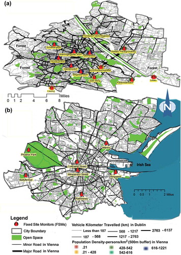
PM₁₀ data were collected using a gravimetric instrument, or analyzed gravimetrically from sampled volumes of air in Dublin area, whereas fine dust samplers were applied in Vienna (Vienna City Administration, 2006; Ireland Environmental Protection Agency, 2014). The average daily PM₁₀ concentrations across the Vienna FSMs were 29.8 and 24.7 µg/m³ for the years 2011 and 2012, respectively, whereas the average daily PM₁₀ concentrations for Dublin were 15.6, 14.7, and 13.8 µg/m³ for the years 2007, 2008, and 2009. Both the Municipal Government of Vienna and the Irish Environmental Protection Agency follow internal quality assurance procedures in order to maintain the highest quality of data and to meet European Union (EU) standards. In Vienna, 1% of FSM data were missing for 2012 and 2% of data were missing for the 2011–2012 period, whereas 6% of data were missing from the seven FSMs and 2% of the data were missing from five FSMs in the period of 2007–2009 in Dublin. For 2009, less than 1% PM₁₀ data were missing from the five FSMs. In addition, some further data were excluded where data on associated independent variables (e.g., weather) were also missing, or contained unexpected values. For Dublin 7, an additional 3.5% of data were missing, due to missing daily peak hour traffic data. Due to missing data among predictor variables in the Vienna data sets, the 2012 and 2011–2012 periods were reduced by 1% and 2%, respectively. Less than 0.05% of data were removed due to unexpected values.

Predictor variables representing differing factors for the area surrounding FSMs were collected from various sources in GIS format. Different buffer zones were established around each FSM, considering the dispersion characteristics of the pollutant in question. These values were determined using ArcGIS software.

In order to estimate vehicle kilometers traveled (VKT), annual average daily traffic (AADT) volume was multiplied by the length of road. VKT surrounding each of the FSMs was determined for different sizes of buffer (100–350 m radius). The AADT data were obtained from the Traffic Noise & Air Quality Unit of Dublin City Council (DCC) in GIS format. In addition, daily traffic count at the nearest junction to the FSMs was also obtained from real-time loop detectors (Sydney Coordinated Adaptive Traffic Systems [SCATS]) in Dublin. Whereas VKT in a buffer provides an indication of the spatial variation of the average traffic, SCATS data may provide additional information about temporal variation at the sites. Daily peak traffic for each intersection was estimated as an average count during morning peak (7–9 a.m.) and evening peak (4–6 p.m.).

Road length data for Dublin was obtained from DCC, whereas the OpenStreetMap (OSM) data set was used for Vienna. Roads that were above the tertiary category were classified as major roads. Land use GIS data sets were obtained from the European central database system (European Environment Agency [EEA], 2013a) and OpenStreetMap (OSM, 2013). Some land use layers of the GIS land use data sets for Dublin and Vienna were combined and reclassified based on their general spatial relationships with ambient air quality. These were (a) pollutant-producing land use—industrial and commercial land use (Dublin), and (b) noncontributing land use—open space (and similar use) in Vienna and Dublin.

Population densities for Dublin were collected from the Central Statistics Office (CSO, 2013) and from the European central database system for Vienna (EEA, 2013b). Dublin meteorological data were combined from both Phoenix Park and Airport stations operated by Met Éireann. Vienna data were obtained from the Schwechat-Flughafen station and were validated against the 2012 data set of Hohe Warte station (ZAMG, 2013). Natural log-transformed wind variables were applied in all of the relevant models as their distribution was positively skewed, and the Anderson-Darling test confirmed that these data did not have a normal distribution.

Air mass history

In an attempt to improve model accuracy, a means of describing the origins of the air mass was included in model Dublin 7. Previous investigations applied wind back-trajectory analysis in identifying the sources of pollutants (Lee et al., 2013). To extend this concept to the current LUR-based modeling framework representing a known source of PM₁₀, the air history was determined using the Hybrid-Single Particle Lagrangian Integrated Trajectory (HYSPLIT) model (National Oceanic and Atmospheric Administration Air Resources Laboratory [NOAA ARL], 2013). The air mass history of 365 days in Dublin in 2009 were determined at a fixed hour of the day (12 p.m.). Each individual air mass history produced by the HYSPLIT model in the form of a trajectory was then overlaid onto a grid developed to produce a rating score indicating the likely degree of pollutant sources it encountered in the previous 48 hr (e.g., Atlantic Ocean vs. UK or northern Europe). Each trajectory was estimated for 48 hr backward in time, as PM₁₀ has been reported to survive for approximately 2 days in the atmosphere (World Health Organization [WHO], 2006). The receptor height was chosen as 500 m, representative of the typical mixing height in Ireland and above ground level to avoid topographic friction (Donnelly, 2011a). The resulting air mass history ratings were subsequently included in the regression for Dublin 7 as the predictor variable D₁.

Figure 2 illustrates the grid developed to carry out the rating of air mass history in the northwestern Europe region. The grid resolution was approximately 54 km², and due to the computational resources available this was the lowest grid size that could be accommodated during this study. Each grid cell was rated based on the average population density range using Europe wide population density data (Center for International Earth Science Information Network [CIESIN], 2013). The rating represented the level of urbanization in respect to a lower threshold of urbanization, as areas with population densities higher than 150 persons/km² are classified as urban (Organisation for Economic Co-operation and Development [OECD], 1994). For population densities below 150 persons/km², grid cells have been divided into five groups having a rating of 1 to 5. Grid cells with population densities greater than 150 persons/km² were equally sized, and an increase in the rating of 1 corresponded to an increase of mean population density of 375 persons/km². Grids predominately occupied by water bodies, or the ocean, were rated as 0.

Figure 2. Air mass history rating grid based on population density and urbanization.

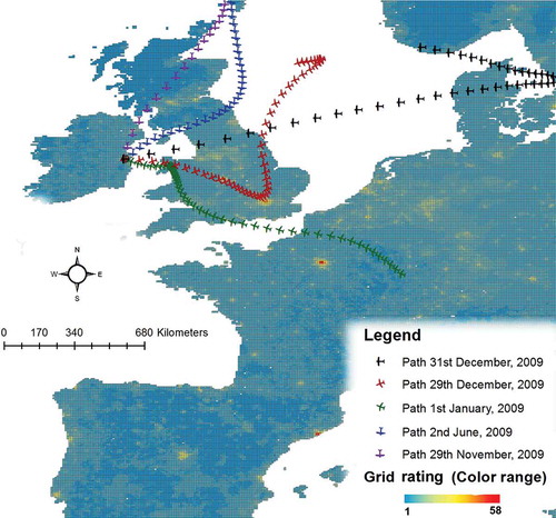
The values of each cell that an individual trajectory passed through were summed to give an accumulative score to each trajectory. Relative to one another, these scores gave an indication of the extent of transboundary air pollution in Dublin for each day in 2009.

Multiple linear regression

The models developed using the MLR statistical technique were of the form shown in eq 1.

(1)

where E is the average daily PM₁₀ concentration; X_i is the predictor variable i; is the error; and A_i is the regression coefficient for predictor variable i.

To develop the MLR models (Vienna 1–3, Dublin 1, 2, and 5–7), the forward selection procedure was applied where predictor variables with the highest simple correlation with the dependent variable were included step by step (Pardoe, 2012). At the end of each step, the variable influential factor (VIF) was checked to ensure no multicollinearity existed, and only statistically significant variables were retained in the models. Normality, tests for all the models were conducted that confirmed an unbiased and homoscedastic relationship between residual and fitted values. In addition, Cook’s distance was checked for outliers and influential variables. The data were checked before model development using scatter plots to ensure that there were no missing values or unexpected values in the analysis. Selected variables (√) in the final models were presented in Table 2.

As MLR assumes that the input data are normally distributed, natural logarithm transformation of PM₁₀ data was carried out in all models. Both the Kolmogorov-Smirnov and Shapiro-Wilk tests for normality in the data confirmed the need for this transformation.

Nonparametric regression

NPR in the form of locally weighted scatter plot smoothing (LOWESS) was also conducted in this study. LOWESS operates by fitting simple models to localized subsets of the data to develop a function that describes the determining part of the variation in the data, point by point. A smooth curve through a set of data points is obtained where each smoothed value is given by a weighted least squares regression. At each point in the data set a low-degree polynomial is fitted to a subset of the data, with explanatory variable values near the point whose response is being estimated. The polynomial is fitted using weighted least squares, giving more weight to points near the point whose response is being estimated (i.e., neighboring points) and less weight to points further away. The value of the regression function for the point is then obtained by evaluating the local polynomial using the explanatory variable values for that data point (Pitard et al., 2004).

The size of the localized subsets or bandwidth was carried out in LOWESS using the k-nearest neighbor approach, and this was optimized during model development by trial and error. The k-nearest neighborhood size for Dublin and Vienna in the final models produced were 35% and 50%, respectively.

Predictor variables for each neighboring point were given a weight through the tricube weighting function. A weighted least-square model was also developed for each point, using only the nearest neighbor observations to minimize the weighted residual sum of the squares. The procedure was carried out for each point, and finally the fitted values were connected to produce the LOWESS curve. A smoothing factor was also required in order to make a balance between bias and prediction noise. Cross-validation was applied to select smoothing factors for each model.

This LOWESS modeling technique of NPR was deployed for Vienna 4 and Dublin 3 . A higher smoothing factor, which was derived by cross-validation, was used for Dublin (0.6) compared with Vienna (0.3) in order to produce better prediction for the Phoenix Park observations. The Phoenix Park is the largest green space in a major city in Europe where the average pollutant concentration during this study was notably lower (11.01 µg/m³) over the three years than the rest of the FSMs in Dublin (15.60 µg/m³).

Artificial neural networks

ANN models were also developed for Vienna 5 and Dublin 4. ANN modeling is an information processing paradigm that is based on the way in which biological nervous systems, such as the brain, process information. In their general form, ANNs refer to parallel model architecture capable of performing numerical calculations based on distributed processing. A feed-forward neural network was used in this study that comprises an input layer, a hidden layer, and an output layer. This ANN operates through each layer, receiving a weighted input from a preceding layer and then transmitting its outputs to neurons in the next layer. The summation of weighted input signals is calculated, and this summation is then transferred by a nonlinear activation function. In this optimization, the Levenberg-Marquardt backpropagation technique was applied, which is widely used for nonlinear least square regressions.

After several iterations with different numbers of hidden neurons (10, 15, 20, 25, 30, and 35), a best-performing network architecture for each city was selected. The combination of “input–hidden layers–output” for Dublin (15-20-1-1) and (15-15-1-1) for Vienna yielded consistent satisfactory results (i.e., similar training and validation performance) for several iterations.

Model validation

Model validation was carried out using the “leave-one-out cross-validation” (LOOCV) technique, whereby one FSM was left out of model development and the model developed was then used to predict the average daily PM₁₀ concentration at the remaining FSMs (Wang et al., 2012). For n FSMs, this process was repeated n times such that each FSMs was excluded in turn from model development and was subsequently used to compare model predictions with measured values.

The comparison of model predictions and measured values was carried out using model performance statistics such as the coefficient of determination (R²) and the root mean square error (RMSE). Comparison of model predictions and measured values was also carried out in two phases, first comparing the model predictions of the measured values included in model development with the same measured values, and second comparing model predictions with measured values excluded from model development using the LOOCV technique. In the case of ANNs, models were developed using 70% of the available input data, while 15% were used for validation and 15% were used for testing.

The development of the standard LUR models was performed using R statistical software (Fox and Weisberg, 2011; R Core Team, 2012). Alternative modeling techniques were developed using Microsoft Excel XLSTAT 2013 suit for nonparametric regression and MATLAB (MathWorks, Natick, MA, USA) for neural networks.

Mapping of ambient air quality

The final models in both cities can be applied at any location for prediction of ambient PM₁₀ concentration, and are applied here on a moderate grid size for discussion. Maps of Dublin and Vienna both were divided into a 400 × 400 m grid and PM₁₀ concentrations were predicted using the final models developed at the centroid of the each grid cell for a typical day in winter. Ordinary kriging was subsequently applied to these data to interpolate between data points and produce maps of ambient PM₁₀ concentrations for both cities. This was carried out using ArcMap 10.1 software (ESRI, 2012).

Results

MLR-based models

The models produced using the MLR statistical technique are shown in Table 3. The baseline model for Vienna was developed with one year’s data and included 13 FSMs (Vienna 1). This model produced an R² of 35%. Increasing the length of historical input data in Vienna 2 from one to two years demonstrated a marginal improvement in R² (37%) and highlighted the stability of the modeling techniques’ predictive performance over the medium term, as has been found by previous investigators (Gulliver et al., 2011; Gonzales et al., 2012). Finally, the addition of seasonal and weekly variation using dummy variables for Vienna resulted in a further marginal improvement in R² to 39%.

Table 3. MLR models for Dublin and Vienna

Model	Variables with ≤0.001 Significance	Adjusted R^2*	P	SE	N	Max.VIF
Vienna 1	Ln(PM) = 5.041 + 2.543 × 10^−2V1 − 8.970 × 10^−2V2 + 8.233 × 10^−6 V3 − 1.935 × 10^−2V4 − 3.475 × 10^−2V5 − 6.869 × 10^−1 V6	0.35	<2.2 × 10^−16	0.47	4624	1.08
Vienna 2	Ln(PM) = 4.906 + 3.242 × 10^−2V1 − 9.933 × 10^−2V2 + 6.304 × 10^−6 V3 − 2.098 × 10^−2V4 − 3.925 × 10^−2V5 − 5.936 × 10^−1V6	0.37	<2.2 × 10^−16	0.47	9264	1.10
Vienna 3	Ln(PM) = 4.707 + 3.242 × 10^−2V1 − 9.934 × 10^−2V2 + 6.321 × 10^−6V3 − 1.599 × 10^−2V4 − 3.667 × 10^−2V5 − 6.061 × 10^−1V6 + 1.682 × 10^−1Winter + 7.794 × 10^−2Tuesday + 1.275 × 10^−1 Wednesday + 1.569 × 10^−1Thursday + 3.743 × 10^−2Friday − 3.339 × 10^−2Saturday − 9.908 × 10^−2Sunday	0.39	<2.2 × 10^−16	0.46	9264	1.28
Dublin 1	Ln(PM) = 2.630 + 4.107 × 10^−6D3 − 1.002 × 10^−1D6 − 9.688 × 10 ^−3D7 − 4.763 × 10^−1D8 − 4.169 × 10^−2 D9 + 2.363 × 10^−1D5	0.39	<2.2 × 10^−16	0.41	5503	1.78
Dublin 2	Ln(PM) = 2.485 + 4.016 × 10^−6D3 − 1.032 × 10^−1D6 − 8.901 × 10^−3D7 − 4.953 × 10^−1D8 − 3.002 × 10^−2D9 + 2.118 × 10^−1D5 + 1.915 × 10^−1Winter + 8.677 × 10^−2 + Tuesday + 9.783 × 10^−2Wednesday + 1.310 × 10^−1Thursday + 1.115 × 10^−1Friday + 4.332 × 10^−2 Saturday − 8.700 × 10^−2Sunday	0.42	<2.2 × 10^−16	0.42	5503	1.33
Dublin 5	Ln(PM) = 2.736 + 4.090 × 10^−6D3 − 8.648 × 10^−2D6 − 4.964 × 10^−1D8 − 4.433 × 10^−2D9 + 2.108 × 10^−1D5	0.39	<2.2 × 10^−16	0.41	4116	1.93
Dublin 6	Ln(PM) = 2.968 + 4.042 × 10^−6D3 − 3.212 × 10^−1D5 − 4.243 × 10^−1D8 − 4.549 × 10^−2D9 + 1.207 × 10^−1D5	0.38	<2.2 × 10^−16	0.40	1624	1.75
Dublin 7	Ln(PM) = 3.071 + 4.936 × 10^−4D1 + 7.297 × 10^−6D2 + 4.904 × 10^−5D4 − 4.554 × 10^−1D8 − 4.288 × 10^−2D9	0.43	<2.2 × 10^−16	0.43	1273	1.61

With a similar performance to Vienna, Dublin 1 was found with R² = 39%. Applying the seasonal variable increases the R² to 42%. Model prediction stability over time could also be noticed when a comparison is made between Dublin 1, Dublin 5, and Dublin 6.

Decreasing the number of FSMs available in 2009 in Dublin 5 resulted in a marginal reduction in model performance (42% to 39%) and again demonstrated the stability of the technique over time. This slight decrease in performance using one year’s data has also been noticed as happened similar in Vienna.

In short, Dublin 2 with the addition of temporal variations showed an increase of model performance similar in magnitude to the increase for Vienna, 4% in both cases.

Using the same five FSMs and including a representation of air mass history and peak traffic count improved performance compared with Dublin 6, with an R² of 43% (Dublin 7). Individually, air mass history was found to explain 6.5% of the variation in PM₁₀, whereas peak traffic count accounted for 12.7%.

NPR and ANN models

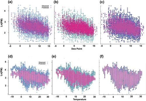
The results of models developed using the proposed alternative statistical modeling techniques are shown in Table 4. The NPR approach in Dublin 3 provided a small improvement of 3% over Dublin 2; however, a significant improvement of 12% was found for Vienna. Models using the ANN approach in Dublin and Vienna produced the highest performance statistics of all models examined at 51% and 66%, respectively. A graphical representation of the results has also been included in Figure 3, showing the predictability of the different modeling techniques. In Figure 3a–f, log-transformed PM₁₀ predicted data were plotted against observed data for a single predictor in the MLR, NPR, and ANN models for Vienna and Dublin, respectively. Figure 3 shows that ANN has predicted data coverage higher than that of the other two models for both Vienna and Dublin.

Table 4. Nonparametric and neural network models for Dublin and Vienna

Model	Model Structure	R^2	No. of Data points
Vienna 4	LOWESS method, polynomial degree: 1; k-nearest neighbors: % = 50; kernel: tricube; bandwidth: standard deviation; smoothing factor: 0.1	0.51	9264
Vienna 5	Two layer Levenberg-Marquardt backpropagation (network structure 15-15-1-1)	0.66	7875
			(85%* of 9264)
Dublin 3	LOWESS method, polynomial degree: 1; k-nearest neighbors: % = 35; kernel: tricube; bandwidth: standard deviation; smoothing factor: 0.6	0.45	5503
Dublin 4	Two layer Levenberg-Marquardt backpropagation (network structure 15-20-1-1)	0.51	4678
			(85%* of 5503)

Notes: *70% for model training and 15% data of model generalization, which also ensured stop training before overfitting.

Figure 3. Graphical representation of the performances of different models. MLR (Vienna 3), (b) NPR (Vienna 4), (c) ANN (Vienna 5), (d) MLR (Dublin 2), (e) NPR (Dublin 3), and (f) ANN (Dublin 4) models.

Model validation results

The results of model cross-validation using the LOOCV technique are shown together with the performance of the models in predicting the measured data involved in their original development in Table 5. As could be expected, the models’ ability to predict the measured data using the LOOCV technique is less than that were predictions are made on the data used for model development. However, in most cases this reduction in performance is marginal with the exception of Dublin 1 and Dublin 2. Both of these models produced poor predictions for the Phoenix Park FSM, which as noted earlier, was significantly different in nature to the other six FSMs in the study. Diem and Comrie (2002) noted that although FSMs are located in unique positions, LOOCV may provide unreliable predictions at most of the monitors, as each monitor may have critically important values for many of the independent variables.

Table 5. Results from model validation

		SD			RMSE
Model	No. of Sites	PM10 (µg/m^3)	Model R^2	ValidationR^2	PM10(µg/m^3)
Vienna 1	13	15.77	0.35	0.36	12.96
Vienna 2	13	17.83	0.37	0.38	14.46
Vienna 3	13	17.83	0.39	0.39	14.36
Vienna 4	13	17.83	0.51	0.48	13.05
Vienna 5	13	17.83	0.66	0.65	10.69
Dublin 1	7	9.18	0.39	0.28	8.17
Dublin 2	7	9.18	0.42	0.30	8.07
Dublin 3	7	9.18	0.45	0.39	7.33
Dublin 4	7	9.18	0.51	0.54	6.27
Dublin 5	5	8.92	0.39	0.35	7.32
Dublin 6	5	7.80	0.38	0.37	6.28
Dublin 7	5	7.52	0.43	0.34	6.28

Again, model predictions using the NPR and ANN techniques produced the best model performance statistics, where Vienna 5 produced the most reliable PM₁₀ predictions.

Discussion

MLR-based models

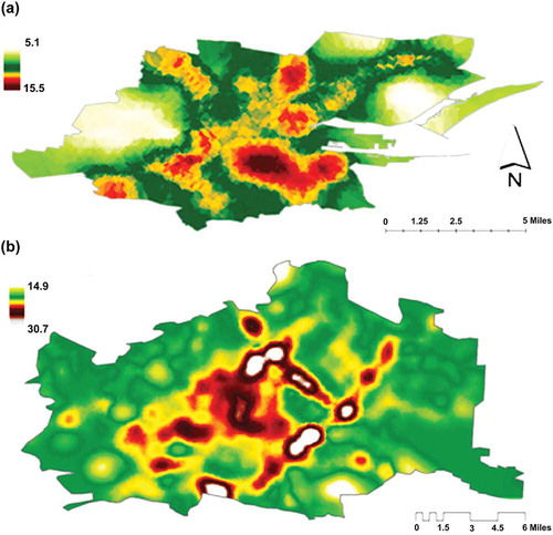
The objective of air pollution modeling in this case is to enable the prediction of air pollution concentrations over large areas with good temporal and spatial resolution, and to do so using the available resources without the need for additional expensive monitoring. Figure 4 shows the results of this process as a typical graphical output for the best-performing models in the study, Vienna 5 and Dublin 4 for a typical winter day. Figure 4b shows similarity in graphical output of the model developed in a recent study Kurz et al. (2014). Kurz et al. (2014) applied a combined emission–dispersion model system to project PM₁₀ concentrations in Vienna between 2005 and 2020, and a graphical representation of the model in 2010 showed that higher PM₁₀ concentration areas were also modeled as high PM₁₀ concentration areas under this study in a typical winter day.

Figure 4. Graphical outputs of average daily PM₁₀ concentrations from (a) Dublin 6 and (b) Vienna 5 for winter Mondays.

With the limited number of FSMs available in Dublin and Vienna, using the MLR approach predictive performance was typically in the range of R² = 28–43%. Such a performance can be considered low and perhaps highlights the limitation of this approach with limited input data. However, it should be noted that in practice FSM data are limited in number, as local government authorities have limited resources with which to measure urban air quality. Thus, air pollution models must be developed to make reliable predictions on air quality using the amount of readily available data, if the problem highlighted at the start of this paper is to be practically addressed.

Using the MLR statistical approach and predictor variables of Dublin 7 produced the R² = 43%, and these can be attributed to the addition of two new variables representing air mass history and peak traffic count. In addition, it can also be noted that the performance of the models across two distinctly different European cities is quite consistent. Omitting Dublin 7 from the result of MLR models gives a range of performance statistics of R² = 30–38%. Furthermore, the stability of predictions from these models over time has been shown to be consistent in both Dublin and Vienna, i.e., little change in performance statistics were noted when the amount of historical input data was increased by one to two years.

The omission of two FSMs in Dublin 5 produced an increase in performance for the model validation data (R² = 0.35 against R² = 0.30 in Dublin 2), which was due to the ability of models developed excluding the Phoenix Park FSM to subsequently make predictions of concentrations at this station. As noted earlier, the Phoenix Park FSM was significantly different in nature to the other six, and the models developed produced very poor predictions of concentration at this location during validation.

In addition, increasing the length of historic input in the Vienna 2 model showed the stability of the modeling techniques, which has also been found by previous investigators (Gulliver et al., 2011; Gonzales et al., 2012). However, the increasing variation (i.e., higher standard deviation) of the data yields a higher RMSE in Table 5 in comparison with the Vienna 1. Previous models were developed based on one year’s data and were applied to consecutive years; on the other hand, models under this study were developed with two or three years’ data together, which led to a larger RMSE. This limitation of RMSE has subsequently tackled by using NPR and ANN methods. The Dublin 5 model was developed following the Dublin 1 model methodology and showed both improvement in model performance and RMSE; however, data variability in the Dublin 5 model was lower than that of Dublin 1 model both in the spatial and temporal sense.

NPR and ANNs

Using the alternative statistical modeling approaches to relate PM₁₀ concentration to the predictor variables produced more favorable results. Using the NPR approach in both Dublin and Vienna, the validation coefficient of determination was at or close to 50%. Using ANNs produced the best predictive performance statistics, with R² of 65% for Vienna and close to 50% for Dublin, and the lowest RMSE for both cities. This highlights the impact of the nonlinear nature of the relationships between many of the variables and PM₁₀ and the assumption of normality in the data for MLR. Thus, using the same number of FSMs and the same historical input data, very significant improvements in model performance can be achieved using a nonlinear statistical technique, regardless of the limited availability of FSM data.

Previous investigations using advanced statistical models have also found that these have outperformed linear regression–based techniques (Chaloulakou et al., 2003). Here, the improvements found were greater for Vienna than for Dublin. For example, a 12% improvement was found using the NPR technique for Vienna, whereas only 3% improvement was found for Dublin. Similarly, a 27% improved was found for Vienna using the ANN technique, whereas this was only 9% for Dublin. This may be explained by the differing characteristics of the two cities and the impact of the respective predictor variables. The sensitivity index for each variable in each city is shown in Supplemental Table A, and shows that the most important variable in Vienna was precipitation, followed by max sustained wind speed. In Dublin it can be seen that the sensitivity index was more evenly distributed across the predictor variables. Comrie (1997) noted that the relationships between air pollution and weather are typically complex and non linear. Therefore as weather variables were of more importance in Vienna than in Dublin the addition of non linear statistical techniques in Vienna have achieved a greater level of improvement than those in Dublin

Air mass history

The representation of air mass history as variable D₁ (in Dublin 7) demonstrated an increase in model performance over the Dublin 6 from 38% to 43%. This finding highlights that LUR-based model predictive performance may be increased significantly with the inclusion of a variable representing the contribution of transboundary air pollution.

The methodology applied here to the derivation of D₁ is a first attempt at the inclusion of such a variable and offers considerable scope for refinement and possible improvement in its explanatory power. Alternative rating systems, including negative scores for water bodies or green areas, could be investigated. Similarly, the density of the grid applied to the derivation may also offer scope for improvement. Other factors that may alter the eventual score attained by a trajectory include the selected height and hour of the day, etc.

Future research is required to examine the optimum approach to the derivation of D₁, and the extent to which improvements in its explanatory power are possible. The inclusion of different ratings for areas with the large combustion plants or sources of natural dust, e.g., ploughing and grazing activities, could be incorporated within the grid for improvements in this model. Such improvement may provide interesting comparison where applied in inland cities and cities where urban background PM₁₀ concentration are heavily influenced by long-range transport and secondary aerosols (Lenschow et al., 2001).

It should also be noted that the production of 365 air mass histories for 2009 and the subsequent production of a rating score for each one was a labor-intensive process in the current study. Future work may also be required to address the automation of this process for wider use in air pollution modeling.

Hourly traffic count

Different forms of traffic volume/intensity data have been used in many previous investigations of the LUR modeling technique. These included annual average daily traffic count (Briggs et al., 2000; Mölter et al., 2010) and simulated traffic data (Jason et al., 2008; Smith et al., 2011; Dons et al., 2013). In the present study, annual average daily traffic data have also been used to derive the VKT variable for models Dublin 1–6. Although data representing annual average daily traffic, or derived variables such as VKT count, often become a useful parameter for incorporating spatial variability in models, hourly traffic count, such as applied in Dublin 7, obtained from the intelligent traffic management systems, i.e., loop detectors, may provide additional temporal information for high-resolution LUR-based models. Such inclusions may be required for the modeling of air quality variations in the shorter term for road users. Annual average traffic count may not always be useful for this purpose, because traffic variability is unpredictable, and traffic causing higher emissions often originate from outside the study area, or the city (Sider et al., 2013).

Conclusions

In conclusion, the results of this investigation highlight that it is possible to predict air pollution concentrations using adaptions of the land use methodology to an acceptable level of accuracy using a limited number of FSMs. It has been shown that this is best achieved using nonlinear statistical modeling techniques such as NPR or ANNs and that this methodology is applicable in two differing cities in Europe. It can also be concluded that the results of the models are stable from year to year in the medium term.

For the purpose of the practical implementation of citywide air pollution models by local authorities, policy makers, or planners, this finding has positive impacts. As highlighted at the outset of this paper, there is a need for air pollution models that can be developed in the absence of additional costly monitoring, over and above the normal level of monitoring carried out by local governments. The proposed methodology highlighted in this paper may facilitate the development of such models.

The proposed addition of transboundary air pollution and a more accurate representation of traffic activity, as predictor variables, have been shown to significantly improve the performance of MLR-based land use regression approach.

Future research is required into the performance of this modeling technique for other forms of air pollution.

Funding

This research was part funded by the European Union 7th Framework Programme under the Peacox Project.

Supplemental Material

Supplemental data for this article can be accessed at http://dx.doi.org/10.1080/10962247.2015.1006377.

Nomenclature

FSM	=	fixed-site monitor
MLR	=	multiple linear regression
LUR	=	land use regression
NPR	=	nonparametric regression
ANN	=	artificial neural network
VKT	=	vehicle kilometer traveled
AADT	=	annual average daily traffic

Acknowledgment

The authors would like to thank Dublin City Council for the provision of input data.

Additional information

Notes on contributors

Md. Saniul Alam

Md. Saniul Alam is a Ph.D. researcher at Trinity College Dublin, Ireland.

Aonghus McNabola

Aonghus McNabola, Ph.D., is an assistant professor of the Department of Civil, Structural and Environmental Engineering, Trinity College Dublin, Ireland.

References

- Abdul-Wahab, S.A., C.S. Bakheit, and S.M. Al-Alawi. 2005. Principal component and multiple regression analysis in modelling of ground-level ozone and factors affecting its concentrations. Environ. Model. Softw. 20:1263–1271. doi:10.1016/j.envsoft.2004.09.001
- Arian, M.A., R. Blair, N. Finkelstein, J.R. Brook, T. Sahsuvaroglu, B. Beckerman, L. Zhang, and M. Jerrett. 2007. The use of wind fields in a land use regression model to predict air pollution concentrations for health exposure studies. Atmos. Environ. 41:3453–3464. doi:10.1016/j.atmosenv.2006.11.063
- Briggs, D.J., C. de Hoogh, J. Gulliver, J. Wills, P. Elliott, S. Kingham, and K. Smallbone. 2000. A regression-based method for mapping traffic-related air pollution: Application and testing in four contrasting urban environments. Sci. Total Environ. 253:151–167. doi:10.1016/S0048-9697(00)00429-0
- Chaloulakou, A., G. Grivas, and N. Spyrellis. 2003. Neural network and multiple regression models for PM10 prediction in Athens: A comparative assessment. J. Air Waste Manage. Assoc. 53:1138–1190. doi:10.1080/10473289.2003.10466276
- Center for International Earth Science Information Network (CIESIN). 2013. Gridded Population of the World (GPW), version 3. http://sedac.ciesin.columbia.edu/gpw (accessed April 2, 2013).
- Chen, C., C. Wu, H. Yu, C. Chan, and T. Cheng. 2012a. Spatiotemporal modelling with temporal-invariant variogram subgroups to estimate fine particle matter PM2.5 concentraions. Atmos. Environ. 54:1–8. doi:10.1016/j.atmosenv.2012.02.015
- Chen, L., Z. Bai, S. Kong, B. Han, Y. You, X. Ding, S. Du, and A. Liu. 2010. A land use regression for predicting NO2 and PM10 concentrations in different seasons in Tianjin region, China. J. Environ. Sci. 22:1364–1373. doi:10.1016/S1001-0742(09)60263-1
- Chen, L., Y. Wang, P. Li, Y. Ji, S. Kong, Z. Li, and Z. Bai. 2012b. A land use regression model incorporating data on industrial point source pollution. J. Environ. Sci. 24:1251–1258. doi:10.1016/S1001-0742(11)60902-9
- Cobourn, W.G., L. Dolcine, M. French, and M.C. Hubbard. 2000. A comparison of non-linear regression and neural network models for ground-level ozone forecasting. J. Air Waste Manage. Assoc. 50:1999–2009. doi:10.1080/10473289.2000.10464228
- Comrie, A.C. 1997. Comparing neural networks and regression models for ozone forecasting. J. Air Waste Manage. Assoc. 47:653–663. doi:10.1080/10473289.1997.10463925
- Central Statistics Office. 2013. Census 2011 Small Area Population Statistics (SAPS). http://www.cso.ie/en/census/census2011smallareapopulationstatisticssaps/ (accessed January 14, 2015).
- Diem, J.E., and A.C. Comrie. 2002.Predictive mapping of air pollution involving sparse spatial observations. Environ. Pollut. 119:99–117. doi:10.1016/S0269-7491(01)00308-6
- Donnelly, A., B.D.R. Misstear, and B. Broderick. 2011a. Relationship of background NO2 concentrations in air to back trajectories through parametric and nonparametric regression methods: Application at two background sites in Ireland. J. Environ. Model. Assess. 17:363–373.
- Donnelly, A., B.D.R. Misstear, and B. Broderick. 2011b. Application of nonparametric regression methods to study the relationship between NO2 concentrations and local wind direction and speed at background sites. Sci. Total Environ. 409:1134–1144. doi:10.1016/j.scitotenv.2010.12.001
- Dons, E., M. Van Poppel, L. Int Panis, S. De Prins, P. Berghmans, G. Koppen, and C. Matheeussen. 2014. Land use regression models as a tool for short, medium and long term exposure to traffic related air pollution. Sci. Total Environ. 476–477:378–386. doi:10.1016/j.scitotenv.2014.01.025
- Dons, E., M. Van Poppel, B. Kochan, G. Wets, and L. Int Panis. 2013. Modeling temporal and spatial variability of traffic-related air pollution: Hourly land use regression models for black carbon. Atmos. Environ. 74:237–246. doi:10.1016/j.atmosenv.2013.03.050
- ESRI (Environmental Systems Resource Institute). 2012. Arc-GIS: ArcMap 10.1. ESRI, Redlands, California. http://www.esri.com/news/arcnews/spring12articles/introducing-arcgis-101.html, (accessed January 15, 2013).
- European Environment Agency. 2013a. Corine land cover 2006 seamless vector data and population density disaggregated with Corine land cover 2000. http://www.eea.europa.eu/data-and-maps/data/clc-2006-vector-data-version-2 (accessed on January 2, 2013).
- European Environment Agency. 2013b. Population density. http://www.eea.europa.eu/data-and-maps/data/population-density#tab-european-data (accessed on January 2, 2013); http://www.eea.europa.eu/data-and-maps/data/population-density#tab-methodology (accessed January 3, 2013).
- Freund, R.J., W.J. Wilson, and P. Sa. 2006. Regression Analysis: Statistical modelling of a Response Variable, 2nd ed. London: Academic Press.
- Fox, J. and S. Weisberg. 2011. An {R} Companion to Applied Regression, Second Edition. Thousand Oaks CA: Sage. http://socserv.socsci.mcmaster.ca/jfox/Books/Companion (accessed January 20, 2013).
- Gonzales, M., O. Myers, L. Smith, H.A. Olvera, S. Mukerjee, W.W. Li, N. Pingitore, M. Amaya, S. Burchiel, M. Berwick, and ARCH Study Team. 2012. Evaluation of land use regression models for NO2 in El Paso, Texas, USA. Sci. Total Environ. 432:135–142. doi:10.1016/j.scitotenv.2012.05.062
- Gulliver, J., K. de Hoogh, D. Fecht, D. Vienneau, and D. Briggs. 2011. Comparative assessment of GIS-based methods and metrics for estimating long-term exposures to air pollution. Atmos. Environ. 45:7072–7080. doi:10.1016/j.atmosenv.2011.09.042
- Hoek, G., R. Beelen, K. de Hoogh, D. Vienneau, J. Gulliver, P. Fischer, and D. Briggs. 2008. A review of lands regression models to assess the spatial variation of outdoor air pollution. Atmos. Environ. 42:7561–7578. doi:10.1016/j.atmosenv.2008.05.057
- Ibarra-Berastegui, G., A. Elias, A. Barona, J. Saenz, A. Ezcurra, and J. Diaz de Argandõna. 2008. From diagnosis to prognosis for forecasting air pollution using neural network: Air pollution monitoring in Bilbao. Environ. Modell. Softw. 23:622–637.
- Ireland Environmental Protection Agency. 2015. Air Quality. http://www.epa.ie/air/quality/ (accessed January 14, 2015).
- Ireland Environmental Protection Agency. 2014. Air quality. http://www.epa.ie/pubs/reports/air/quality/aqreview2010.html#.VFN2oPmsVig 2/3 (accessed November 1, 2014).
- Jason, G.S., M. Brauer, B. Ainslie, D. Steyn, T. Larson, and M. Buzzelli. 2008. An innovative land use regression model incorporating meteorology for exposure analysis. Sci. Total Environ. 390:520–529.
- Kurz, C., R. Orthofer, P. Sturm, A. Kaiser, U. Uhrner, R. Reifeltshammer, and M. Rexeis. 2014. Projection of the air quality in Vienna between 2005 and 2020 for NO2 and PM10. Urban Climate 10(4):703–719. doi:10.1016/j.uclim.2014.03.008
- Lee, S., C.-H. Ho, Y.G. Lee, H.J. Choi, and C.K. Song. 2013. Influence of transboundary air pollutants from China on the high-PM10 episode in Seoul, Korea for the period October 16−20, 2008. Atmos. Environ. 77:430–439. doi:10.1016/j.atmosenv.2013.05.006
- Lenschow, P., H.-J. Abraham, K. Kutzner, M. Lutz, J.-D. Preuß, and W. Reichenbächer. 2001. Some ideas about the sources of PM10. Atmos. Environ. 35(Suppl. 1):S23–S33. doi:10.1016/S1352-2310(01)00122-4
- MacIntyre, E.A., C.J. Karr, M. Koehoorn, P.A. Demers, L. Tamburic, C. Lencar, and M. Brauer. 2011. Residential air pollution and otitis media during the first two years of life. Epidemiology 22:81–89. doi:10.1097/EDE.0b013e3181fdb60f
- McNabola, A., B.M. Broderick, and L.W. Gill. 2009. A principal components analysis of the factors effecting personal exposure to air pollution in urban commuters in Dublin, Ireland. J. Environ. Sci. Health A 44:1–9. doi:10.1080/10934520903139928
- Mölter, A., S. Lindley, F. de Vocht, A. Simpson, and R. Agius. 2010. Modelling air pollution for epidemiologic research—Part II: Predicting temporal variation through land use regression. Sci. Total Environ. 409:211–217. doi:10.1016/j.scitotenv.2010.10.005
- National Oceanic and Atmospheric Administration Air Resources Laboratory. 2013. HYSPLIT—Hybrid Single Particle Lagrangian Integrated Trajectory Model. http://ready.arl.noaa.gov/HYSPLIT.php (accessed February 12, 2013).
- Organisation for Economic Co-operation and Development. 1994. Creating Rural Indicators For Shaping Territorial Policy. Paris: Organisation for Economic Co-operation and Development.
- OpenStreetMap. 2013. OpenStreetMap: Data extracts. http://download.geofabrik.de/europe.html (accessed January 2, 2013).
- Pardoe, I. 2012. Applied Regression Modelling, 2nd ed. New York: Wiley & Sons.
- Pitard, A., A. Zeghnoun, A. Courseaux, J. Lamberty, V. Delmas, J. Luc Fossard, and H. Villet. 2004. Short term associations between air pollution and respiratory drug sales. Environ. Res. 95:43–52. doi:10.1016/j.envres.2003.08.006
- R Core Team. 2012. R: A language and environment for statistical computing. R Foundation for Statistical Computing, Vienna, Austria. http://www.R-project.org/ (accessed January 1, 2013).
- Sahsuvaroglu, T., A. Arain, P. Kanaroglou, N. Finkelstein, N. Newbold, M. Jerrett, B. Beckerman, J. Brook, M. Finkelstein, and N.L. Gilbert. 2012. A land use regression model for predicting ambient concentrations of nitrogen dioxide in Hamilton, Ontario, Canada. J. Air Waste Manage. Assoc. 56:1059–1069. doi:10.1080/10473289.2006.10464542
- Sider, T., A. Alam, M. Zukari, H. Dugum, N. Goldstein, N. Eluru, and M. Hatzopoulou. 2013. Land-use and socio-economics as determinants of traffic emissions and individual exposure to air pollution, J. Transport Geogr. 33:230–239. doi:10.1016/j.jtrangeo.2013.08.006
- Smith, L.A., S. Mukerjee, K.C. Chung, and J. Afgani. 2011. Spatial analysis and land use regression of VOCs and NO2 in Dallas, Texas during two seasons. J. Environ. Monit. 13:999–1007. doi:10.1039/c0em00724b
- Vienna City Administration. 2006. Vienna Environmental Report 2004/2005. http://www.wien.gv.at/english/environment/protection/reports/pdf/complete-report-04.pdf (accessed November 1, 2014).
- Wang, M., R. Beelen, M. Eeftens, K. Meliefste, G. Hoek, and B. Brunekreef. 2012. Systematic evaluation of land use regression models for NO2. Environ. Sci. Technol. 46:4481–4489. doi:10.1021/es204183v
- World Health Organization. 2006. Health risks of particulate matter from long-range transboundary air pollution: Joint WHO/Conventation Task Force on the Health Aspects of Air Pollution. http://www.euro.who.int/__data/assets/pdf_file/0006/78657/E88189.pdf (accessed January 12, 2013).
- Yann, S., J. Galineau, A. Hulin, F. Caini, N. Marquis, V. Navel, S. Bottagisi, L. Giorgis-Allemand, C. Jacquier, R. Slama, and J. Lepeule. 2014. Health effects of ambient air pollution: Do different methods for estimating exposure lead to different results? Environ. Int. 66:165–173.
- ZAMG (Zentralanstalt für Meteorologie und Geodynamik). 2013. Central Institute for Meteorology and Geodynamics, Vienna, e-mail correspondence, April 11, 2013.