An assessment of air pollutant exposure methods in Mexico City, Mexico

Abstract

Geostatistical interpolation methods to estimate individual exposure to outdoor air pollutants can be used in pregnancy cohorts where personal exposure data are not collected. Our objectives were to a) develop four assessment methods (citywide average (CWA); nearest monitor (NM); inverse distance weighting (IDW); and ordinary Kriging (OK)), and b) compare daily metrics and cross-validations of interpolation models. We obtained 2008 hourly data from Mexico City’s outdoor air monitoring network for PM₁₀, PM_2.5, O₃, CO, NO₂, and SO₂ and constructed daily exposure metrics for 1,000 simulated individual locations across five populated geographic zones. Descriptive statistics from all methods were calculated for dry and wet seasons, and by zone. We also evaluated IDW and OK methods’ ability to predict measured concentrations at monitors using cross validation and a coefficient of variation (COV). All methods were performed using SAS 9.3, except ordinary Kriging which was modeled using R’s gstat package. Overall, mean concentrations and standard deviations were similar among the different methods for each pollutant. Correlations between methods were generally high (r = 0.77 to 0.99). However, ranges of estimated concentrations determined by NM, IDW, and OK were wider than the ranges for CWA. Root mean square errors for OK were consistently equal to or lower than for the IDW method. OK standard errors varied considerably between pollutants and the computed COVs ranged from 0.46 (least error) for SO2 and PM10 to 3.91 (most error) for PM2.5. OK predicted concentrations measured at the monitors better than IDW and NM. Given the similarity in results for the exposure methods, OK is preferred because this method alone provides predicted standard errors which can be incorporated in statistical models. The daily estimated exposures calculated using these different exposure methods provide flexibility to evaluate multiple windows of exposure during pregnancy, not just trimester or pregnancy-long exposures.

Implications: Many studies evaluating associations between outdoor air pollution and adverse pregnancy outcomes rely on outdoor air pollution monitoring data linked to information gathered from large birth registries, and often lack residence location information needed to estimate individual exposure. This study simulated 1,000 residential locations to evaluate four air pollution exposure assessment methods, and describes possible exposure misclassification from using spatial averaging versus geostatistical interpolation models. An implication of this work is that policies to reduce air pollution and exposure among pregnant women based on epidemiologic literature should take into account possible error in estimates of effect when spatial averages alone are evaluated.

Introduction

Air pollution is a major public health problem, with growing numbers of urban residents living in areas with air pollution levels exceeding the World Health Organization (WHO) air quality guidelines (Cohen et al., 2005). Air pollution has been associated with mortality and morbidity (Borja-Aburto et al., 1997; Brunekreef and Holgate, 2002), cardiovascular disease (Künzli et al., 2005; Park et al., 2008), and adverse pregnancy outcomes (e.g., low birth weight, preterm birth, intrauterine growth retardation) (Slama et al., 2008; Woodruff et al., 2009).

Many previous epidemiological studies of air pollution have used data collected from central monitoring sites (Ozkaynak et al., 2013). Recent advances in the availability of fine-resolution remote sensing data and application of methods that incorporate temporal and spatial variability have demonstrated that exposure measurement error from the use of central sites can influence pollutant-specific health effects estimates (Ozkaynak et al., 2013). Several publications on outdoor air pollution and perinatal outcomes have used birth registries and air pollution data from government-run air quality monitors to create exposure estimates (Bell et al., 2007; Chang et al., 2012; Sagiv et al., 2005). Other exposure assessment approaches (Jerrett et al., 2004) include methods that account for the mother’s residential location (Nethery et al., 2008), proximity to traffic or other sources of emission (Wilhelm and Ritz, 2003; Yorifuji et al., 2011), land-use regression models (Brauer et al., 2008; Slama et al., 2007), models to reduce exposure measurement error (Zou et al., 2009), and even personal monitoring of mothers during pregnancy (Jedrychowski et al., 2005; Perera et al., 2005; Perera et al., 2009).

The spatial distribution of air pollutants gives rise to special considerations in exposure assessment methods. For instance, spatial averaging of air pollution (i.e., averaging concentrations across all monitors in a given area or city) may adequately represent individual exposures to spatially homogeneous pollutants (Brunekreef and Holgate, 2002). Alternatively, when the study participants’ location is known or if exposures decline with distance from a pollution source due to mixing and dilution effects, other methods can be used. Nearest monitor, inverse distance weighting, and ordinary Kriging use distance to estimate exposure to outdoor air pollution. (Brauer et al., 2008; Janssen et al., 2001; Wyler et al., 2000). In particular, Kriging is an interpolation technique that estimates values at unsampled locations based on concentrations sampled spatially (e.g., a network of monitors within an urban area) and has been used for exposure estimates (Iñiguez et al., 2009; Jerrett et al., 2005; Leem et al., 2006; Liao et al., 2006; Ross et al., 2013; Shad et al., 2009). Additionally, Kriging allows calculation of uncertainty in the estimated values, essential to quantify the potential bias caused by air pollution exposure measurement error (Gryparis et al., 2009; Marshall et al., 2008; Woodruff et al., 2009).

Although interpolation methods have many advantages, no published studies to our knowledge have used them to estimate individual air pollution exposure in Mexico City, a place with significant air pollution and one of the world’s top 10 mega-cities. We used 2008 daily ambient air pollution data from metropolitan Mexico City to construct and compare different exposure assessment methods (citywide average [CWA], nearest monitor [NM], inverse distance weighting [IDW], and ordinary Kriging [OK]) for application in perinatal epidemiology studies where mothers’ residential locations are known. The differences among these methods were evaluated in a simulated population from various regions of metropolitan Mexico City. We compared daily predicted air pollutant concentrations for this population by various methods to guide assessment of associations between air pollution and preterm birth in a mother–infant pair cohort recruited from 1994 to 2005 (Ettinger et al., 2008), and for an ongoing study in Mexico City (O´Neills et al., 2013).

Methods

Study location

The Federal District of Mexico (Mexico City) has an estimated population of 8.9 million (INEGI, 2010) and is located in a valley surrounded by mountains reaching elevations of 2,240 m above sea level. The area is impacted by pollution sources ranging from industrial refineries to traffic emissions and wind-blown dust from a dry lake basin. Although the metropolitan area often meets daily standards for six regulated pollutants (carbon monoxide [CO], particulate matter with aerodynamic diameter ≤ 10 and 2.5 µm, respectively [PM₁₀; PM_2.5], ozone [O₃], sulfur dioxide [SO₂], and nitrogen dioxide [NO₂]), it does not meet the annual standards, with concentrations almost double the limits for many pollutants (Hamilton et al., 2013). The Mexico City air quality standards are as follows: PM₁₀ (annual mean: 50 μg/m³; daily average: 120 μg/m³); PM_2.5 (annual mean: 15 μg/m³; daily average: 65 μg/m³); O₃ (1-hr average: 110 ppb; 8-hr average: 80 ppb); SO₂ (annual mean: 30 ppb; daily average: 130 ppb); NO₂ (1-hr average: 210 ppb); CO (8-hr average: 11 ppm).

Air pollution data

The air quality monitoring network in Mexico City (“Sistema de Monitoreo Atmosférico,” SIMAT by its acronym in Spanish) provides hourly data on the six pollutants from 34 stations. Of these 34 sites, 22 sample for O₃; 26 for SO₂; 18 for NO₂; 18 for CO; 14 for PM₁₀; and 9 for PM_2.5 (Zuk et al., 2007). We downloaded the data on April 19, 2011, for the whole calendar year of 2008 from the SIMAT website (http://www.sma.df.gob.mx). We chose 2008 because this is a relatively recent year with measurements representative of improvements to the network and validation methods, but also a year that has had adequate time for any corrections to be made. Prior to posting on the website, SIMAT staff clean and validate the data (A. Retama-Hernandez personal communication, 2011; Zuk et al., 2007). PM₁₀ and PM_2.5 were reported in micrograms per cubic meter (µg/m³), whereas O₃, CO, NO₂, and SO₂ were reported in parts per million (ppm). O₃, NO₂, and SO₂ data were transformed from parts per million to parts per billion (ppb) to facilitate comparison of concentration levels with Mexico City air pollution standards. PM₁₀, PM_2.5, and CO retained the originally reported units. Although data are available hourly for most pollutants, we summarized data as daily concentrations (24-hr averages) for particulates (PM₁₀ and PM_2.5), SO₂, and NO₂, and the daily 8-hr maximum running average for CO and O₃, from all available monitoring stations. These concentration averaging times match the Mexican health-based regulatory standards (Zuk et al., 2007). If more than 25% of the hourly values in a given day were missing, the daily concentration was coded as “missing.” The term “daily value” or “pollutant concentration” refers to these summaries.

Simulated population location data for exposure estimation

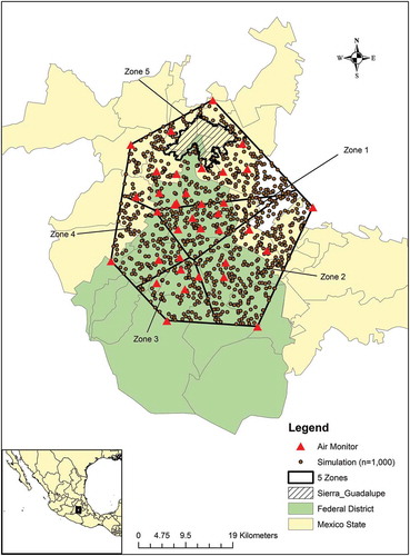
Our goal was to construct and compare exposure metrics and eventually assign them to participants in a pregnancy cohort in Mexico (O´Neill et al., 2013). To evaluate these metrics, we simulated a population of 1,000 women with residential locations distributed across the metropolitan area. To restrict the area of simulated residences to a zone within which we could perform Kriging, we created a polygon surrounding the perimeter of the entire air monitoring network (i.e., the convex hull) using ArcGIS 9.3.1 (ESRI, Redlands, CA) (Figure 1). Then we mapped the location of five monitoring stations at which we also deployed our own equipment and sampled particulate matter for toxicological and chemical compositional evaluation (Manzano-León et al., 2013). These locations also informed our recruiting of participants for our pregnancy cohort study (Vadillo-Ortega et al., 2014), and enabled us to divide Mexico City into north, south, east, west, and center zones with potentially distinct pollution sources and mixtures. Thiessen polygons, which describe “areas of influence” within which any given location is closer to its corresponding monitor than any of the other four monitors, were created to subdivide the convex hull into five zones surrounding these stations (Figure 1). The Hawth’s Tools extension to ArcGIS (Beyer, 2004) was used to generate 200 random locations according to population density (from Mexico City’s 2005 census data, http://www.inegi.org.mx) within each of the five polygons, omitting areas known to be uninhabited or where people probably do not live (e.g., parks, industrial, nonresidential areas). This simulation mimics the spatial distribution of potential future study participants.

Figure 1. Location of simulated subjects’ residences, Thiessen polygons, and air quality monitors in Mexico City.

Exposure Assessment Methods

Citywide averaging (CWA)

Citywide or spatial averaging uses a simple average of a given pollutant across all monitors within an identified geographic region to estimate an individual’s exposure. Estimates thus will not reflect spatial gradients of concentration that may be present for certain air pollutants. Previous studies have used spatial averaging as a surrogate of personal exposure to outdoor pollution (Borja-Aburto et al., 1998; Brunekreef and Holgate, 2002).

Nearest monitor (NM)

The NM method assigns pollutant concentration at the closest monitor to the study participant’s location as the exposure estimate. We defined distance as the shortest straight line from the air quality monitor to the simulated residential location using ArcGIS 9.3.1 Hawth’s Tools (Beyer, 2004). The NM method relied on the three closest neighboring monitors, in case the nearest monitor was missing data for any given day. In that scenario, data from the second or the third closest monitor was used.

Inverse distance weighting (IDW)

IDW computes predicted concentrations at a location as a weighted average of concentrations at neighboring monitors. Weights are a function of the inverse of the distance between the location and each monitor; for example, 1/distance⁵ or 1/distance². Higher values of the power applied to the inverse distance emphasize the contribution of the nearest points to the location and interpolated values. The higher the value of the exponent, the less influence from distant points is exerted. We selected the square of the inverse distance (1/distance²) to create a smoother surface across simulated locations. The square is also one of the default parameters commonly used in this method. We used at least five monitors closest to the residence location to calculate the IDW exposure estimates, with a maximum of 12 monitors for each pollutant.

Ordinary Kriging (OK)

Several forms of Kriging (simple Kriging, block Kriging, universal Kriging, ordinary Kriging) have been used to estimate air pollution exposure (Brauer et al., 2008; Leem et al., 2006; Wong et al., 2004). Similar to IDW, OK calculates a weighted average of concentrations at monitoring stations to estimate a participant’s exposure. However, OK uses weights derived from a function of distance referred to as a variogram, which describes the degree of spatial dependence or autocorrelation. A positive-definite model of the variogram is fitted to a plot of semivariance (a measure of deviation between pairs of sample points) and distance, calculated from observed data. OK assumes that the variogram model describing the spatial dependence is constant across the region being mapped.

The OK operation yields a continuous surface of estimated pollution concentrations within a defined geographical area, which can be mapped to grid cells. At any given location or grid cell, the value of the surface (i.e., a predicted concentration for the location) can be estimated, along with its estimation variance (or standard error). The standard error will be lower for points closer to the actual monitors, since the standard error represents the estimation error due to location, sampling error, and measurement error. An advantage of OK over other interpolation methods is that the weights assigned to the data are computed to minimize the standard error, whereas IDW assigns weights to neighboring locations in a way that is not informed by the observed spatial correlation of the sampled data (i.e., the variogram).

Variogram modeling

Spherical, Gaussian, and exponential models were used to model the variogram. R statistical software (version 2.12.1) and the gstat package (Pebesma, 2004; Szpiro et al., 2010) were used to estimate the optimal model parameters. Because variogram parameters are affected by positive skewness in the air pollution data, data were log-transformed to facilitate estimation. Results from the spherical model are presented because it had the lowest root mean squared error (RMSE), described later, meaning it fit the empirical variogram best. The nugget, which is related to the short-range variability of the data due to measurement error, was set to zero.

Creating the metrics

Daily exposure estimates for calendar year 2008 were constructed for all 1,000 locations using the exposure methods above described. Because outdoor pollution in Mexico City, a relatively temperate climate, varies seasonally, we used rainy (May through October) or dry season (November through April) periods for calculating longer term averages and comparing exposure metrics, in addition to year-long summary calculations.

Statistical Analysis

We produced descriptive statistics on daily measured pollutant concentrations in 2008 and the exposure estimates, overall; by season; and by region. For the OK estimates, we chose to assign a concentration and its corresponding standard error for a given pollutant only to those residences within each pollutant-specific polygon, because outside these polygons, the method is essentially extrapolating, and standard errors are generally large. We then calculated Pearson correlation coefficients among pollutants for 2008 based on pollutant daily values, and for each pollutant, correlations were then calculated daily across exposure assessment methods for each of the 1,000 locations, both citywide and in five zones. The mean differences in exposure estimates across methods for the 200 participants in each of the five Thiessen polygons (zones) were also calculated to assess regional differences and method performance.

Model evaluation

We compared CWA, IDW, and NM methods to OK by computing the absolute value of the difference between each method and OK, and by comparing root mean square error (RMSE) of the estimated values from the NM and IDW to the OK estimates’ RMSEs. In theory, estimates of air pollution exposure produced by Kriging better reflect spatial variability and provide a proxy of individual-level exposure with less measurement error than the other three methods. Thus, in subsequent comparisons we used the values and variances of the Kriging estimates as the point of reference for comparing the performance of each method, in the absence of a true “gold standard” (measured concentration at the location of simulated participants’ homes).

Kriging offers an additional opportunity for evaluating potential error in estimating pollution exposure, since the standard error of the OK estimate reflects estimation error due to location, sampling error, and measurement error. Regarding measurement error, comparisons between personally monitored exposures and ambient monitor data indicate that fine particles are more spatially homogeneous than gaseous pollutants and thus better represent overall exposure (Sarnat et al., 2009). Air pollutants with fewer sample points (so average distance is greater, increasing error due to location) would have higher standard errors, on average, for the Kriging estimates. The Kriging standard error also depends on the nugget, so pollutants with higher measurement/sampling error (we cannot be sure what the nugget is representing) would also have greater overall standard errors when summarized across all the estimates, and give an indication of which pollutants are harder to estimate with spatial interpolation. To evaluate whether some pollutants had more estimation error than others, we calculated a version of a coefficient of variation for each of the six pollutants by dividing the mean of the daily-predicted Kriging standard errors by the standard deviation of all the Kriging-estimated daily pollution concentrations. This ratio can be thought of as the proportion of the variance in the estimated pollutant due to measurement, location, and sampling error (vs. true variation), and the higher the dimensionless number, the greater is the error associated with the estimated pollutant concentration (Shechtman, 2013).

Finally, we used cross-validation to assess the performance of interpolation methods. In cross-validation, commonly referred to as the “leave-one-out” approach, each sampling site was removed from the data set one at a time, and the remaining data were used to predict the pollutant concentration at that particular site. The predicted value for the monitor was then compared to the true observed value at that site. Equation 1 was used to compute RMSE from the daily cross validations was used to compare method performance and precision in terms of predicting the monitored concentration:

2 (1)

where is the estimated pollutant concentration at location i; is the air pollutant concentration at location i; and n is the number of pollutant-specific monitoring sites, which varies depending on the pollutant. An RMSE of zero means the prediction of the parameter of interest (air pollution concentration) matches the observation perfectly, although such values are practically impossible to achieve.

The Statistical Analysis System (SAS version 9.3; SAS Institute, Inc., Cary, NC) was used for estimating CWA, NM, and IDW concentrations, whereas R, Version 2.11.0, package gstat (Pebesma, 2004), was used for estimating OK.

Results

Table 1 presents summary descriptive statistics for the four air pollutant metrics estimated for the 1,000 simulated study participants during all of 2008 and within the dry and wet seasons. Overall, means and standard deviations from the different methods were similar within each pollutant across the 2008 study period. However, the ranges of estimated concentrations determined by NM, IDW, and OK were always wider than the ranges for CWA. Seasonally, days with maximum pollutant concentrations occurred during the dry season for all exposure assessment methods. Overall, estimated pollutant concentrations, with the exception of SO₂ and CO, sometimes surpassed air quality standards established by U.S. and Mexican regulations.

Table 1. Descriptive statistics for four exposure metrics calculated for 1,000 simulated residents of Mexico City using daily concentrations of air pollutants during calendar year 2008

		Entire year 2008		Dry season^a		Wet season^b
Pollutant (monitors)	Method	Mean ± (SD)^c	Range	Mean ± (SD)^c	Range	Mean ± (SD)^c	Range
PM10 (µg/m^3)	CWA	53.2 (20.6)	14.4–109.7	67.8 (15.4)	20.7–109.7	38.8 (13.9)	14.4–88.0
14 Sites	NM	53.7 (25.4)	8.0–214.1	68.9 (23.8)	15.1–214.1	38.7 (16.6)	8.0–122.5
	IDW	54.1 (22.6)	8.2–209.8	68.8 (19.2)	15.3–209.7	39.4 (15.2)	8.2–120.6
	OK	52.9 (22.8)	8.4–206.7	67.8 (19.5)	15.7–206.7	38.1 (14.8)	8.4–113.2
PM2.5 (µg/m^3)	CWA	26.8 (10.1)	7.7–67.0	32.4 (8.3)	9.2–67.0	21.4 (8.7)	7.7–52.5
9 Sites	NM	27.6 (13.0)	4.5–110.3	33.7 (12.5)	6.2–110.3	21.6 (10.5)	4.5–91.3
	IDW	27.4 (11.3)	4.6–110.2	33.1 (10.0)	6.2–110.2	21.7 (9.4)	4.6–91.1
	OK	26.3 (10.0)	5.6–102.4	31.6 (8.2)	6.5–102.4	21 (8.6)	5.6–82.6
O3 (ppb)	CWA	58.0 (18.5)	12.7–113.3	61.6 (16.5)	22.7–98.3	54.4 (19.6)	12.7–113.3
22 Sites	NM	56.8 (21.3)	3.50–160.3	60.5 (20)	3.50–127.4	53.1 (21.9)	4.0–160.3
	IDW	56.9 (19.6)	4.5–151.5	60.6 (17.7)	4.50–124.7	53.3 (20.6)	4.7–151.5
	OK	56.6 (19.0)	5.4–134.5	60.3 (17.1)	6.70–127.3	52.9 (20.0)	5.4–134.5
NO2 (ppb)	CWA	30.6 (9.3)	10.7–62.4	35.6 (9.4)	16.1–62.4	25.7 (6.0)	10.7–48.8
18 Sites	NM	30.3 (10.9)	3.2–79.2	35.0 (11.2)	3.50–79.2	25.7 (8.2)	3.2–70.7
	IDW	31.4 (9.9)	3.6–78.6	36.2 (10.0)	4.20–78.6	26.6 (7.1)	3.6–70.0
	OK	29.7 (10.0)	3.5–78.9	34.8 (9.9)	4.80–78.9	24.7 (7.0)	3.5–70.0
CO (ppm)	CWA	1.54 (0.58)	0.40–3.45	1.88 (0.58)	0.55–3.45	1.21 (0.36)	0.44–2.30
17 Sites	NM	1.57 (0.75)	0.07–5.47	1.92 (0.76)	0.09–5.47	1.22 (0.56)	0.07–3.59
	IDW	1.59 (0.63)	0.08–5.39	1.92 (0.64)	0.13–5.39	1.26 (0.44)	0.08–3.53
	OK	1.50 (0.60)	0.20–5.00	1.90 (0.60)	0.20–5.00	1.20 (0.4)	0.10–3.6
SO2 (ppb)	CWA	6.67 (5.12)	2.29–33.9	8.00 (6.10)	2.50–33.9	5.37 (3.45)	2.29–22.1
26 Sites	NM	6.38 (6.30)	1.00–164.3	7.50 (7.58)	1.00–164.3	5.27 (4.41)	1.00–49.1
	IDW	6.56 (5.65)	1.02 – 163.0	7.82 (6.76)	1.02–163.0	5.32 (3.90)	1.00–46.3
	OK	6.00 (5.3)	0.91–153.0	7.00 (6.3)	1.00–153.0	4.90 (3.7)	0.90–43.3

Notes: ^aDry season (November–April); ^bWet season (May–October); ^cStandard deviation.

Maximum PM₁₀ concentrations were higher in northern Mexico City, and O₃ concentrations were higher in the south. By contrast, PM_2.5 concentrations were spatially invariant. All other pollutants had a relatively low level of spatial variation across the area and across estimates produced for the overall study period (data not shown).

The correlation coefficients across pairs of exposure methods and all air pollutants were generally high (0.77 to 0.99; Table 2). As expected, the two weighted averaging methods, IDW and OK, were the most highly correlated. NM correlations with other methods were always the smallest, since no averaging with data from other monitors is employed in that method. All pollutant estimates produced by CWA, with the exception of SO₂, were highly correlated with OK estimates.

Table 2. Pearson correlation coefficients among four metrics estimating the exposure of 1,000 simulated women to six different air pollutants in Mexico City, 2008

	CWA (N)	NM (N)	IDW (N)
		PM10
NM	0.83
IDW	0.92	0.95
OK	0.92	0.94	0.98
		PM2.5
NM	0.83
IDW	0.93	0.95
OK	0.99	0.84	0.94
		O3
NM	0.85
IDW	0.94	0.95
OK	0.96	0.91	0.97
		NO2
NM	0.82
IDW	0.93	0.94
OK	0.93	0.91	0.97
		CO
NM	0.77
IDW	0.91	0.92
OK	0.94	0.85	0.96
		SO2
NM	0.77
IDW	0.88	0.95
OK	0.83	0.93	0.97

Note: All p values <0.05; N values range from 140,910 to 319,860, due to missing data and OK estimates being restricted to locations within pollutant specific polygons.

The strength of the correlations across pairs of exposure methods varied across five zones depicted in Figure 1. Supplemental Table S-1(a–f) shows Pearson correlation coefficients between exposure assessment methods for each air pollutant for the five zones. Correlation coefficients were relatively high between methods for all pollutants, except for between CWA and NM. In all except the southern zone, CO showed high correlations between methods (r values ranging from 0.77 to 0.96). NO₂ exhibited high correlations between methods, except for CWA and NM, for all zones. Correlation coefficients for O₃ estimated by CWA and NM in the north and center zones were relatively lower than for other zones. Methods had high correlations for PM₁₀ and PM_2.5, when all zones were examined, although for PM_2.5, the CWA, NM, and OK methods had lower correlations in the southeast and west zones. Lastly, methods were less correlated for SO₂ in the southeast, south, west, and northwest zones than for other pollutants, where CWA had higher correlation with IDW than with either NM or OK.

Table 3 shows the mean and standard deviations of differences in estimates by method, using OK as the “gold standard,” across all pollutants and zones. In northern Mexico City (zone 5, with typically high PM₁₀ levels), CWA and IDW underestimated PM₁₀ on average, relative to OK, by 4.17 µg/m³ and 1.80 µg/m³, respectively, and NM overestimated the exposure by 4.11 µg/m³ when compared to OK. In the south (zone 3), CWA overestimated PM₁₀ exposure by 7.49 µg/m³, whereas NM and IDW underestimated the exposure by 3.09 µg/m³ and 7.21 µg/m³, respectively. IDW produced lower standard deviations of the mean difference for the north and south zones. The center and eastern zones (zones 1 and 2, respectively) exhibited minimal differences in PM₁₀ estimates for the four methods. For PM_2.5, methods produced relatively similar results across zones. In the southern zone (high O₃), CWA underestimated the exposure by 0.91and IDW by 3.29 ppb, whereas NM overestimated the exposure by 4.18 ppb. IDW estimates produced higher standard deviations of the mean difference between methods. Applied to NO₂, CO, and SO_2, all three methods produced similar estimates. Estimates produced by IDW showed higher standard deviations than other methods.

Table 3. Mean differences and standard deviations (SD) of the differences in air pollution exposure estimates produced by three exposure assessment methodologies for 1,000 simulated women in Mexico City during 2008, with ordinary Kriging used as reference method

			Mean Difference (SD)
Zone	Model	PM10 (µg/m^3)	PM2.5 (µg/m^3)	O3 (ppb)	NO2 (ppb)	CO (ppm)	SO2 (ppb)
All Zones	CWA	0.34 (9.03)	0.56 (1.04)	1.40 (5.43)	0.88 (3.61)	–0.03 (0.20)	0.71 (3.03)
	NM	0.84 (8.96)	1.36 (7.10)	0.20 (9.06)	0.59 (4.53)	0.02 (0.40)	0.42 (2.44)
	IDW	–2.30 (12.2)	0.38 (5.10)	–2.68 (8.29)	–0.07 (6.02)	–0.10 (0.34)	–0.18 (1.97)
1	CWA	–1.14 (5.83)	0.61 (0.94)	1.94 (4.67	–1.53 (3.77)	–0.11 (0.24)	0.59 (2.19)
	NM	1.75 (7.37)	0.13 (3.57)	–1.30 (8.17)	1.69 (5.07)	0.18 (0.40)	0.21 (2.02)
	IDW	–3.40 (10.8)	–0.12 (3.11)	–2.62 (5.85)	1.03 (3.42)	0.01 (0.22)	–0.27 (1.75)
2	CWA	0.94 (5.52)	0.43 (1.48)	0.97 (4.68	1.05 (2.71)	–0.01 (0.14)	1.57 (2.81)
	NM	0.08 (7.99)	4.95 (10.23)	1.57 (9.25)	1.14 (4.54)	0.08 (0.40)	0.24 (2.15)
	IDW	–2.50 (9.83)	2.46 (7.52)	–4.22 (8.71)	0.19 (6.54)	–0.13 (0.36)	–0.21 (1.71)
3	CWA	7.49 (7.47)	0.76 (0.90)	–0.91 (5.82)	0.72 (3.67)	0.09 (0.24)	0.97 (2.37)
	NM	–3.09 (5.91)	–2.78 (3.87)	4.18 (8.54)	0.94 (4.55)	–0.20 (0.45)	0.41 (1.86)
	IDW	–7.21 (14.0)	–2.31 (3.49)	–3.29 (13.2)	–2.40 (11.1)	–0.30 (0.55)	–0.64 (2.35)
4	CWA	7.26 (7.95)	0.65 (0.49)	–0.23 (4.82)	1.18 (2.83)	0.03 (0.22)	0.18 (2.76)
	NM	–3.62 (6.31)	–0.92 (4.69)	2.56 (7.64)	0.71 (3.28)	0.05 (0.40)	0.64 (2.24)
	IDW	–3.40 (5.57)	–1.22 (2.96)	0.33 (6.4)	0.76 (3.04)	–0.05 (0.26)	0.14 (1.75)
5	CWA	–4.17 (10.5)	0.58 (0.71)	2.83 (6.03)	1.70 (4.02)	0.01 (0.19)	0.12 (3.55)
	NM	4.11 (10.5)	–0.59 (4.24)	–2.39 (9.05)	–0.54 (4.45)	–0.05 (0.32)	0.59 (3.55)
	IDW	–1.80 (15.5)	0.01 (2.84)	–2.30 (7.36)	–0.50 (5.08)	0.10 (0.29)	–0.12 (2.22)

Notes: Zone 1 = Center; Zone 2 = East; Zone 3 = South; Zone 4 = West; Zone 5 = North. Negative values reflect underestimation by the exposure method being compared to ordinary Kriging. Mean differences were calculated as CWA_{concentration} – OK_{concentration} for each day and then averaged for the whole year for each woman, and then the mean and SD across all women were calculated for each pollutant; identical calculations were done for IDW and NM.

Descriptive statistics for all pollutants for individuals who reside within pollutant-specific polygons, along with the standard error and coefficients of variation (COV) for Kriging estimates, are shown in Table 4. The number of participants living within these polygons varies by pollutant, since the number and locations of monitors with available measures (and the corresponding convex hull polygon) of a given pollutant are different. The mean concentrations calculated within these polygons by the study methods were relatively similar to mean concentrations produced for all 1,000 individuals across Mexico City. Maximum concentrations estimated by OK were lower than for the two other interpolation methods, except for NO₂. PM₁₀ and PM_2.5 showed significantly lower predicted maximum concentrations using OK compared to NM and IDW.

Table 4. Descriptive statistics for estimated concentrations of each pollutant for locations inside pollutant specific polygons in 2008 in Mexico City, and standard errors (SE) and coefficient of variation (COV)^a for OK estimates

Pollutant	Method		N	Mean	SD	Range
PM10 (µg/m^3)	CWA		189,222	53.2	20.6	14.4, 109.7
14 Sites	NM		189,210	55.1	25.7	8.0, 214.1
	IDW		189,222	50.6	21.9	8.2, 206.4
	OK		189,222	53.6	22.8	8.4, 194.4
	OK (SE)			10.5		0.5, 66.0
	OK (COV)	0.46
PM2.5 (µg/m^3)	CWA		154,452	26.8	10.1	7.7, 67.0
9 Sites	NM		154,452	27.0	12.0	4.5, 110.3
	IDW		154,452	26.2	10.8	4.6, 108.8
	OK		154,452	26.2	9.9	5.6, 88.2
	OK (SE)			38.7		3.2, 100.0
	OK (COV)	3.9
O3 (ppb)	CWA		319,884	58.0	18.5	12.7, 113.3
22 Sites	NM		319,860	57.1	21.4	3.5, 160.3
	IDW		319,518	53.8	20.0	4.5, 151.5
	OK		319,884	56.7	19.0	5.4, 134.5
	OK (SE)			10.4		0.6, 107.5
	OK (COV)	0.55
CO (ppm)	CWA		140,910	1.54	0.58	0.44, 3.45
17 Sites	NM		140,886	1.66	0.77	0.07, 5.47
	IDW		140,910	1.53	0.68	0.08, 5.39
	OK		140,910	1.58	0.64	0.19, 4.99
	OK (SE)			0.45		0.07, 1.19
	OK (COV)	0.70
NO2 (ppb)	CWA		163,236	30.6	9.3	10.7, 62.4
18 Sites	NM		163,223	32.3	11.6	3.2, 79.2
	IDW		163,236	30.4	10.6	3.6, 78.6
	OK		163,236	31.0	10.4	3.5, 78.9
	OK (SE)			5.0		0.5, 18.0
	OK (COV)	0.48
SO2 (ppb)	CWA		308,904	6.67	5.12	2.29, 33.89
26 Sites	NM		308,461	6.30	6.32	1.00, 16.43
	IDW		308,904	5.72	5.36	1.00, 16.27
	OK		308,904	5.92	5.28	0.09, 15.30
	OK (SE)			2.44		0.11, 53.8
	OK (COV)	0.46

Notes: The sample sizes used to calculate these summary statistics differ by pollutant and method because (1) differing subsets of the 1,000 locations fell inside pollutant-specific polygons (PM₁₀: 517; PM_2.5: 422; O₃: 874; CO: 385; NO₂: 446 and SO₂: 844) and (2) some daily pollutant concentrations were missing on certain days. ^aCoefficient of variation (COV) for OK = (mean standard error of estimates/mean standard deviation of concentrations).

As previously noted, OK produces both a concentration estimate and its corresponding standard error for individuals living within pollutant-specific polygons. The range of the OK standard errors varied considerably between pollutants and the computed coefficients of variation ranged from 0.46 (least error) for SO₂ and PM₁₀ to 3.91 (most error) for PM_2.5, the pollutant with only 9 monitoring sites (Table 4).

Results from the cross-validation are shown in Table 5. The RMSEs for OK were consistently equal to or lower than for the other two methods, and only for non-log-transformed O₃ and NO₂ did IDW have RMSEs equal to those of OK. This suggests that the OK method did the best overall job of predicting the actual measured concentrations at monitoring sites.

Table 5. Root mean square errors (RMSE) by exposure method when data are cross-validated with the actual concentrations measured at Mexico City air pollution monitors during 2008

Pollutant	Exposure method	RMSE	Range^a
PM10 (µg/m^3)	Nearest monitor	0.281	0.092–0.555
14 Sites	IDW	0.226	0.091–0.395
	Ordinary Kriging	0.218	0.077–0.463
PM2.5 (µg/m^3)	Nearest monitor	0.247	0.087–0.738
9 Sites	IDW	0.229	0.076–0.535
	Ordinary Kriging	0.230	0.082–0.508
O3 (ppb)	Nearest monitor	0.320	0.084–1.280
22 Sites	IDW	0.235	0.071–0.710
	Ordinary Kriging	0.210	0.066–0.660
CO (ppm)	Nearest monitor	0.513	0.180–1.220
17 Sites	IDW	0.402	0.153–0.900
	Ordinary Kriging	0.380	0.150–0.890
NO2 (ppb)	Nearest monitor	0.271	0.088–0.598
18 Sites	IDW	0.235	0.080–0.499
	Ordinary Kriging	0.230	0.081–0.510
SO2 (ppb)	Nearest monitor	0.611	0.267–1.010
26 Sites	IDW	0.495	0.285–0.820
	Ordinary Kriging	0.476	0.260–0.900

Note: ^aRange (minimum – maximum).

Discussion

This study compared daily exposure estimates derived from using four exposure assessment methods (CWA, NM, IDW, and OK) for 1,000 simulated women in Mexico City during 2008, to help guide selection of exposure metrics in perinatal epidemiological studies. We evaluated differences in the metrics produced and the accuracy of prediction of actual measured values by descriptive statistics, correlations, and cross-validation statistics. Air pollution exposure assessment in epidemiological studies on birth outcomes has sometimes relied on simple spatial averaging methods for estimation of individual exposure to airborne contaminants; this study provides insights into the extent to which the temporal and spatial variation of air pollution exposures may affect estimated exposure. Estimating exposure by taking location within this megacity into account can reduce the likelihood for exposure misclassification in health studies, increasing power to detect associations by capturing an adequate gradient of exposure in the study population (Navidi et al., 1999).

The four exposure assessment methods yielded similar, but not identical, results for the air pollutants examined. The ranges of exposure estimates produced by methods incorporating location were significantly wider than for estimates produced by CWA. A cohort study in a Korean population utilized exposure assessment methods similar to those of our study and found similar estimates for different air pollutants, and that concentration ranges from methods accounting for geographical location were greater than those from spatial averaging (Son et al., 2010). A study comparing Kriging and nearest monitor methods in estimating health effects associated with long-term pollution exposures concluded that Kriging was generally better due to lower bias and better coverage of health effect parameter estimates. (Kim et al., 2009) In addition, researchers found that different interpolation methods produced similar estimates when monitor density was low, whereas when monitor density was high the differences were much greater (Kim et al., 2009; Wong et al., 2004). High correlation coefficients between OK and IDW in our study suggest that these two interpolation methods were similarly able to predict spatial variation in concentrations of air pollutants in Mexico City, and the cross-validation suggested that IDW was a close second in predictive ability.

Regarding ease of use, the NM and IDW methods are simpler to calculate than OK. Air pollution exposure estimation by OK poses several challenges. One involves empirical and experimental variogram estimation. To automate and optimize the daily estimation of variogram parameters (range, sill, and nugget), skewed air pollution data must be log-transformed (Liao et al., 2006). Also, to select the best fitting model, based on cross validation, variogram parameters needed to be determined by exploring their RMSE values under different covariance models (spherical, exponential, and Gaussian). For all air pollutants, the spherical covariance model showed the lowest RMSE. Similarly, other researchers experimented with model fit and selected the spherical model (Son et al., 2010). In spite of the more labor-intensive calculation, the advantage of Kriging is that standard errors for the estimated exposures can be calculated, unlike for IDW and NM. With these standard errors, one could use inverse variance weighting to give more precise Kriged exposure estimates a greater contribution when estimating epidemiologic associations, or use available measurement error models (Gryparis et al., 2009; Madsen et al., 2008; Spiegelman et al., 2011; Wannemuehler et al., 2009).

We recommend that Kriged exposure estimates be employed in future epidemiological studies in Mexico City. However, one caveat is illustrated by the coefficient of variation calculation we made with the Kriging standard errors and standard deviation. This suggested that estimation error relative to true variance is much greater in the PM_2.5 Kriged estimates than for the other five pollutants. This is likely because PM_2.5 is monitored at only nine sites in Mexico City, and PM_2.5 is known to be a spatially homogeneous pollutant that represents individual exposure well (Sarnat, 2005). Including PM_2.5 estimated by several exposure assessment methods in epidemiologic models may yield relatively consistent effect estimates, or, in other words, the specific exposure metric used for PM_2.5 may be less critical than for other pollutants that have more geographical variation.

Strengths of this study include inclusion and comparison of methods that address both temporal and spatial scales of the air pollution data derived from the monitoring network and the creation of future capacity for linking estimates with an ongoing birth cohort. Moreover, because daily exposure was calculated using different exposure methods, we have the flexibility to construct multiple windows of exposure during pregnancy, not limited to trimesters or overall pregnancy windows, allowing us to capture all the biologically relevant times of exposure. Further, considering that Mexico City is a megacity, geocoding positional errors, more likely in rural settings, are of little concern in our study population or in future geo-referenced data from the city (Ward et al., 2005).

Limitations include the fixed number of available monitors (notably for PM_2.5), because a denser network would improve model performance, and variability in the numbers of reporting monitors by day, which changes the shape of the daily polygon. Additionally, we lacked personal exposure measurements as a gold standard in the simulated locations. However, previous work suggests that outdoor monitor concentrations are well correlated with indoor and personal measures of exposure to air pollution in Mexico City (O’Neill et al., 2003; Rojas-Bracho, 1994). Lastly, polygon shape is defined by the monitors reporting in a given day, and variations in the number and location of these monitors can shift the interpolation area relative to the residence location and increase prediction errors of interpolated data.

Nevertheless, our work adds to the growing literature comparing air pollution exposure assessment methods (Kim et al., 2009; Ross et al., 2013; Szpiro et al., 2011). A logical next step is to link the estimates from these models with health outcomes data to evaluate whether the pollution effect estimates differ by metric used, which may not always be the case (Szpiro et al., 2011; Gryparis, Paciorek et al., 2009; Madsen et al., 2008).

Examining spatial variation in air pollution exposure, especially in Mexico City where “bowl-shape” topography promotes the accumulation of pollutants and the formation of air pollution concentration gradients, is important for epidemiological studies. Earlier and recent studies examining particulate exposure have shown variation by size and chemical composition in different zones within Mexico City (Manzano-León et al., 2013; Osornio-Vargas et al., 2003).

Conclusions

The power of perinatal epidemiology studies in Mexico City can be enhanced by knowing the location where pregnant women spend their time, enabling exposure estimation in both temporal and spatial domains, and thus maximizing exposure contrasts. Second, OK and IDW interpolation methods yielded similar estimated exposures among the simulated residences, so use of these metrics in studies with health outcomes may yield similar associations. If epidemiologic effect estimates do not differ significantly among the four exposure estimation metrics, using OK may be a recommended approach due to the available standard errors. Third, the zone of Mexico City in which women live can affect how well different exposure metrics correlate. This suggests that measurement error may have variable magnitude depending on zone of residence, especially when using a method like CWA.

Application of the exposure estimation methods we described in perinatal epidemiology may help clarify controversies about the role of exposure to air pollutants and the development of specific conditions, such as preterm labor, as limited and inconclusive evidence has been found by researchers (Liu et al., 2003; Simpson et al., 1997; Vadillo-Ortega et al., 2014). However, factors relevant to preterm risk could also differ by zone of residence, so disentangling the contribution of exposure measurement error from confounding by these other factors could present a challenge.

Our plans to combine the estimated exposures from outdoor monitors with biomarker data, reports on personal activities and exposure, and detailed clinical data will improve our ability to understand how air pollution influences perinatal health, in Mexico City and elsewhere, and to set control and prevention priorities.

Funding

This study was supported by US National Institute of Environmental Health Sciences (National Institute of Health [NIH]/NIEHS) grants R01 ES016932-01, R01 ES017022-91, P20 ES018171, P01 ES02284401, and P30 ES017885, Environmental Protection Agency (EPA) grants RD834800 and RD83543601, and by the University of Michigan Center for Global Health and Rackham School of Graduate Studies. We thank Shannon Brines for his insights and assistance provided at the Environmental Spatial Analysis Lab (ESA) at the University of Michigan. This research was supported in part by the Department of Energy, Environmental, and Chemical Engineering, Washington University, St. Louis. The authors would also like to thank the China Section of the Air & Waste Management Association for the generous scholarship they received to cover the cost of page charges, and make the publication of this paper possible. The content of this article is solely the responsibility of the authors and does not necessarily represent the official views of the NIEHS and/or NIH.

Supplemental Materials

Supplemental data for this article can be accessed at http://dx.doi.org/10.1080/10962247.2015.1020974.

Additional information

Funding

This study was supported by US National Institute of Environmental Health Sciences (National Institute of Health [NIH]/NIEHS) grants R01 ES016932-01, R01 ES017022-91, P20 ES018171, P01 ES02284401, and P30 ES017885, Environmental Protection Agency (EPA) grants RD834800 and RD83543601, and by the University of Michigan Center for Global Health and Rackham School of Graduate Studies. We thank Shannon Brines for his insights and assistance provided at the Environmental Spatial Analysis Lab (ESA) at the University of Michigan. This research was supported in part by the Department of Energy, Environmental, and Chemical Engineering, Washington University, St. Louis. The authors would also like to thank the China Section of the Air & Waste Management Association for the generous scholarship they received to cover the cost of page charges, and make the publication of this paper possible. The content of this article is solely the responsibility of the authors and does not necessarily represent the official views of the NIEHS and/or NIH.

Notes on contributors

Luis O. Rivera-González

Luis O. Rivera-González is a research associate in the Department of Energy, Chemical, and Environmental Engineering at Washington University in St. Louis, MO.

Zhenzhen Zhang

Zhenzhen Zhang is a doctoral candidate and Brisa N. Sánchez is an associate professor at the Department of Biostatistics, University of Michigan, School of Public Health, Ann Arbor, MI.

Brisa N. Sánchez

Zhenzhen Zhang is a doctoral candidate and Brisa N. Sánchez is an associate professor at the Department of Biostatistics, University of Michigan, School of Public Health, Ann Arbor, MI.

Kai Zhang

Kai Zhang is an assistant professor in the Division of Epidemiology, Human Genetics, and Environmental Sciences, University of Texas School of Public Health, Houston, TX.

Daniel G. Brown

Daniel G. Brown is a professor in the School of Natural Resources and Environment, University of Michigan, Ann Arbor, MI, and directs the Environmental Spatial Analysis Laboratory.

Leonora Rojas-Bracho

Leonora Rojas-Bracho is an independent consultant in the air pollution field in Mexico City, Mexico.

Alvaro Osornio-Vargas

Alvaro Osornio-Vargas is a physician and researcher in the field of air pollution and toxicology in the Department of Pediatrics, University of Alberta, Edmonton, Alberta, Canada.

Felipe Vadillo-Ortega

Felipe Vadillo-Ortega is a professor at Universidad Nacional Autónoma de México, and a physician and researcher at the Unidad de Vinculación de la Facultad de Medicina, at the Instituto Nacional de Medicina Genómica, Ciudad de México, México.

Marie S. O’Neill

Marie S. O’Neill is an associate professor in the Departments of Environmental Health Sciences and Epidemiology, University of Michigan, School of Public Health, Ann Arbor, MI.

References

- Bell, M. L., K. Ebisu, et al. 2007. Ambient air pollution and low birth weight in Connecticut and Massachusetts. Environ. Health Perspect. 115(7):1118–24. doi:10.1289/ehp.9759
- Beyer, H. L. 2004. Hawth’s Analysis Tools for ArcGIS. http://www.spatialecology.com/htools.
- Borja-Aburto, V. H., M. Castillejos, et al. 1998. Mortality and ambient fine particles in southwest Mexico City, 1993–1995. Environ. Health Perspect. 106(12):849–55. doi:10.2307/3434129
- Borja-Aburto, V. H., D. P. Loomis, et al. 1997. Ozone, suspended particulates, and daily mortality in Mexico City. Am. J. Epidemiol. 145(3):258–68. doi:10.1093/oxfordjournals.aje.a009099
- Brauer, M., C. Lencar, et al. 2008. A cohort study of traffic-related air pollution impacts on birth outcomes. Environ. Health Perspect. 116(5):680–6. doi:10.1289/ehp.10952
- Brunekreef, B. and S. T. Holgate. 2002. Air pollution and health. Lancet 360:1233–42. doi:10.1016/S0140-6736(02)11274-8
- Chang, H. H., B. J. Reich, et al. 2012. Time-to-event analysis of fine particle air pollution and preterm birth: Results from North Carolina, 2001–2005. Am. J. Epidemiol. 175(2):91–98. doi:10.1093/aje/kwr403
- Cohen, A. J., H. Ross Anderson, et al. 2005. The global burden of disease due to outdoor air pollution. J. Toxicol. Environ. Health A 68(13–14):1301–7. doi:10.1080/15287390590936166
- Ettinger, A. S., H. C. Lamadrid-Figueroa, et al. 2008. Effect of calcium supplementation on blood lead levels in pregnancy: A randomized placebo-controlled trial. Environ. Health Perspect. 117(1):26–31. doi:10.1289/ehp.11868
- Gryparis, A., C. J. Paciorek, et al. 2009. Measurement error caused by spatial misalignment in environmental epidemiology. Biostatistics 10(2):258–74. doi:10.1093/biostatistics/kxn033
- Hamilton, B. E., D. L. Hoyert, et al. 2013. Annual summary of vital statistics: 2010–2011. Pediatrics 131(3):548–558. doi:10.1542/peds.2012-3769
- INEGI. 2010. Censo de Poblacion y Vivienda: Estados Unidos Mexicanos Resultados Preliminares. http://www.inegi.org.mx/est/contenidos/proyectos/ccpv/cpv2010/.
- Iñiguez, C., F. Ballester, et al. 2009. Estimation of personal NO2 exposure in a cohort of pregnant women. Sci. Total Environ. 407(23):6093–99. doi:10.1016/j.scitotenv.2009.08.006
- Janssen, N. A. H., P. H. N. van Vliet, et al. 2001. Assessment of exposure to traffic related air pollution of children attending schools near motorways. Atmos. Environ. 35(22):3875–84. doi:10.1016/S1352-2310(01)00144-3
- Jedrychowski, W., A. Galas, et al. 2005. Prenatal ambient air exposure to polycyclic aromatic hydrocarbons and the occurrence of respiratory symptoms over the first year of life. Eur. J. Epidemiol. 20(9):775–82. doi:10.1007/s10654-005-1048-1
- Jerrett, M., A. Arain, et al. 2004. A review and evaluation of intraurban air pollution exposure models. J. Expos. Anal. Environ. Epidemiol. 15(2):185–204. doi:10.1038/sj.jea.7500388
- Jerrett, M., R. T. Burnett, et al. 2005. Spatial analysis of air pollution and mortality in Los Angeles. Epidemiology 16(6):727–36. doi:10.1097/01.ede.0000181630.15826.7d
- Kim, S.-Y., L. Sheppard, et al. 2009. Health effects of long-term air pollution: Influence of exposure prediction methods. Epidemiology 20(3):442–50. doi:10.1097/EDE.0b013e31819e4331
- Künzli, N., M. Jerrett, et al. 2005. Ambient air pollution and atherosclerosis in Los Angeles. Environ. Health Perspect. 113(2):201–6. doi:10.1289/ehp.7523
- Leem, J. H., B. M. Kaplan, et al. 2006. Exposures to air pollutants during pregnancy and preterm delivery. Environ. Health Perspect. 114(6):905–10. doi:10.1289/ehp.8733
- Liao, D., D. Peuquet, et al. 2006. GIS approaches for the estimation of residential-level ambient PM concentrations. Environ. Health Perspect. 114(9):1374–80. doi:10.1289/ehp.9169
- Liu, S., D. Krewski, et al. 2003. Association between gaseous ambient air pollutants and adverse pregnancy outcomes in Vancouver, Canada. Environ. Health Perspect. 111(14):1773–78. doi:10.1289/ehp.6251
- Madsen, L., D. Ruppert, et al. 2008. Regression with spatially misaligned data. Environmetrics 19(5):453–67. doi:10.1002/env.888
- Manzano-León, N., R. Quintana, et al. 2013. Variation in the composition and in vitro proinflammatory effect of urban particulate matter from different sites. J. Biochem. Mol. Toxicol. 27(1):87–97. doi:10.1002/jbt.21471
- Marshall, J. D., E. Nethery, et al. 2008. Within-urban variability in ambient air pollution: Comparison of estimation methods. Atmos. Environ. 42(6): 1359–69. doi:10.1016/j.atmosenv.2007.08.012
- Navidi, W., D. Thomas, et al. 1999. Statistical methods for epidemiologic studies of the health effects of air pollution. Res. Rep. Health Effects Institute 86:1–50.
- Nethery, E., S. E. Leckie, et al. 2008. From measures to models: an evaluation of air pollution exposure assessment for epidemiological studies of pregnant women. Occup. Environ. Med. 65(9):579–86. doi:10.1136/oem.2007.035337
- O’Neill, M. S., M. Ramirez-Aguilar, et al. 2003. Ozone exposure among Mexico City outdoor workers. J. Air Waste Manage. Assoc. 53(3): 339–46. doi:10.1080/10473289.2003.10466156
- O’Neill, M. S., A. Osornio-Vargas, et al. 2013. Air pollution, inflammation and preterm birth in Mexico City: Study design and methods. Sci. Total Environ. 448:79–83. doi:10.1016/j.scitotenv.2012.10.079
- Osornio-Vargas, A. R., J. C. Bonner, et al. 2003. Proinflammatory and cytotoxic effects of Mexico City air pollution particulate matter in vitro are dependent on particle size and composition. Environ. Health Perspect. 111(10):1289–93. doi:10.1289/ehp.5913
- Ozkaynak, H., L. K. Baxter, et al. 2013. Evaluation and application of alternative air pollution exposure metrics in air pollution epidemiology studies. J. Expos. Sci. Environ. Epidemiol. 23(6):565–65. doi:10.1038/jes.2013.50
- Ozkaynak, H., L. K. Baxter, et al. 2013. Air pollution exposure prediction approaches used in air pollution epidemiology studies. J. Expos. Sci. Environ. Epidemiol. 23(6):566–72. doi:10.1038/jes.2013.15
- Park, S. K., M. S. O’Neill, et al. 2008. Air pollution and heart rate variability: Effect modification by chronic lead exposure. Epidemiology 19(1):111–20. doi:10.1097/EDE.0b013e31815c408a
- Pebesma, E. J. 2004. Multivariable geostatistics in S: The gstat package. Comput. Geosci. 30:683–91. doi:10.1016/j.cageo.2004.03.012
- Perera, F., D. Tang, et al. 2005. DNA damage from polycyclic aromatic hydrocarbons measured by benzo[a]pyrene-DNA adducts in mothers and newborns from Northern Manhattan, the World Trade Center Area, Poland, and China. Cancer Epidemiol. Biomarkers Prevent. 14(3):709–14. doi:10.1158/1055-9965.EPI-04-0457
- Perera, F. P., Z. Li, et al. 2009. Prenatal airborne polycyclic aromatic hydrocarbon exposure and child IQ at age 5 years. Pediatrics 124(2):e195–202. doi:10.1542/peds.2008-3506
- Rojas-Bracho, L. 1994. Evaluación del grado de exposición a aeroparticulas en los habitantes de la zona centro de la Ciudad de México. Master’s thesis, Universidad Nacional Autonoma de México, Mexico City, Mexico.
- Ross, Z., K. Ito, et al. 2013. Spatial and temporal estimation of air pollutants in New York City: Exposure assignment for use in a birth outcomes study. Environ. Health 12(1):51. doi:10.1186/1476-069X-12-51
- Sagiv, S. K., P. Mendola, et al. 2005. A time-series analysis of air pollution and preterm birth in Pennsylvania, 1997–2001. Environ. Health Perspect. 113(5): 602–6. doi:10.1289/ehp.7646
- Sarnat, J. A., K. W. Brown, J. Schwartz, B. A. Coull, P. Koutrakis. 2005. Ambient gas concentrations and personal particulate matter exposures: implications for studying the health effects of particles. Epidemiology 16(3):385–95.
- Sarnat, S. E., M. Klein, et al. 2009. An examination of exposure measurement error from air pollutant spatial variability in time-series studies. J. Expos. Sci. Environ. Epidemiol. 20(2):135–46. doi:10.1038/jes.2009.10
- Shad, R., M. S. Mesgari, et al. 2009. Predicting air pollution using fuzzy genetic linear membership kriging in GIS. Comput. Environ. Urban Systems 33(6):472–81. doi:10.1016/j.compenvurbsys.2009.10.004
- Shechtman, O. 2013. The coefficient of variation as an index of measurement reliability. In Methods of Clinical Epidemiology, ed. S. A. R. Doi and G. M. Williams, 39–49. Berlin, Germany: Springer.
- Simpson, R. W., G. Williams, et al. 1997. Associations between outdoor air pollution and daily mortality in Brisbane, Australia. Arch. Environ. Health 52(6):442–54. doi:10.1080/00039899709602223
- Slama, R., L. Darrow, et al. 2008. Atmospheric pollution and human reproduction: Report of the Munich International Workshop. Environ. Health Perspect. 116(6):791–98. doi:10.1289/ehp.11074
- Slama, R., V. Morgenstern, et al. 2007. Traffic-related atmospheric pollutants levels during pregnancy and offspring’s term birth weight: A study relying on a land-use regression exposure model. Environ. Health Perspect. 115(9): 1283–92. doi:10.1289/ehp.10047
- Son, J.-Y., M. L. Bell, et al. 2010. Individual exposure to air pollution and lung function in Korea: Spatial analysis using multiple exposure approaches. Environ. Res. 110(8):739–49. doi:10.1016/j.envres.2010.08.003
- Spiegelman, D., R. Logan, et al. 2011. Regression calibration with heteroscedastic error variance. Int. J. Biostat. 7(1):1–38. doi:10.2202/1557-4679.1259
- Szpiro, A. A., C. J. Paciorek, et al. 2011. Does more accurate exposure prediction necessarily improve health effect estimates? Epidemiology 22(5):680–85. doi:10.1097/EDE.0b013e3182254cc6
- Szpiro, A. A., P. D. Sampson, et al. 2010. Predicting intra-urban variation in air pollution concentrations with complex spatio-temporal dependencies. Environmetrics 21(6):606–31. doi:10.1002/env.1014
- Vadillo-Ortega, F., A. Osornio-Vargas, et al. 2014. Air pollution, inflammation and preterm birth: A potential mechanistic link. Med. Hypoth. 82(2): 219–24. doi:10.1016/j.mehy.2013.11.042
- Wannemuehler, K. A., R. H. Lyles, et al. 2009. A conditional expectation approach for associating ambient air pollutant exposures with health outcomes. Environmetrics 20(7):877–94. doi:10.1002/env.978
- Ward, M. H., J. R. Nuckols, et al. 2005. Positional accuracy of two methods of geocoding. Epidemiology 16(4):542–47. doi:10.1097/01.ede.0000165364.54925.f3
- Wilhelm, M., and B. Ritz. 2003. Residential proximity to traffic and adverse birth outcomes in Los Angeles County, California, 1994–1996. Environ. Health Perspect. 111(2):207–16. doi:10.1289/ehp.5688
- Wong, D. W., L. Yuan, et al. 2004. Comparison of spatial interpolation methods for the estimation of air quality data. J. Expos. Anal. Environ. Epidemiol. 14(5): 404–15. doi:10.1038/sj.jea.7500338
- Woodruff, T. J., J. D. Parker, et al. 2009. Methodological issues in studies of air pollution and reproductive health. Environ. Res. 109(3):311–20. doi:10.1016/j.envres.2008.12.012
- Wyler, C., C. Braun-Fahrländer, et al. 2000. Exposure to motor vehicle traffic and allergic sensitization. Epidemiology 11(4):450–56. doi:10.1097/00001648-200007000-00015
- Yorifuji, T., H. Naruse, et al. 2011. Residential proximity to major roads and preterm births. Epidemiology 22(1):74–80. doi:10.1097/EDE.0b013e3181fe759f
- Zou, B., J. G. Wilson, et al. 2009. Air pollution exposure assessment methods utilized in epidemiological studies. J. Environ. Monit. 11(3):475–90. doi:10.1039/b813889c
- Zuk, M., G. Tzintzun Cervantes, et al. 2007. Tercer almanaque de datos y tendencias de la calidad del aire en nueve ciudades mexicanas. Ciudad de México, Instituto Nacional de Ecología, Mexico City, Mexico.