Estimation of methane emission from California natural gas industry

Abstract

Energy generation and consumption are the main contributors to greenhouse gases emissions in California. Natural gas is one of the primary sources of energy in California. A study was recently conducted to develop current, reliable, and California-specific source emission factors (EFs) that could be used to establish a more accurate methane emission inventory for the California natural gas industry. Twenty-five natural gas facilities were surveyed; the surveyed equipment included wellheads (172), separators (131), dehydrators (17), piping segments (145), compressors (66), pneumatic devices (374), metering and regulating (M&R) stations (19), hatches (34), pumps (2), and customer meters (12). In total, 92,157 components were screened, including flanges (10,101), manual valves (10,765), open-ended lines (384), pressure relief valves (358), regulators (930), seals (146), threaded connections (57,061), and welded connections (12,274). Screening values (SVs) were measured using portable monitoring instruments, and Hi-Flow samplers were then used to quantify fugitive emission rates. For a given SV range, the measured leak rates might span several orders of magnitude. The correlation equations between the leak rates and SVs were derived. All the component leakage rate histograms appeared to have the same trend, with the majority of leakage rates <0.02 cubic feet per minute (cfm). Using the cumulative distribution function, the geometric mean was found to be a better indicator than the arithmetic mean, as the mean for each group of leakage rates found. For most component types, the pegged EFs for SVs of ≥ 10,000 ppmV and of ≥ 50,000 ppmV are relatively similar. The component-level average EFs derived in this study are often smaller than the corresponding ones in the 1996 U.S. Environmental Protection Agency/Gas Research Institute (EPA/GRI) study.

Implications: Twenty-five natural gas facilities in California were surveyed to develop current, reliable, and California-specific source emission factors (EFs) for the natural gas industry. Screening values were measured by using portable monitoring instruments, and Hi-Flow samplers were then used to quantify fugitive emission rates. The component-level average EFs derived in this study are often smaller than the corresponding ones in the 1996 EPA/GRI study. The smaller EF values from this study might be partially attributable to the employment of the leak detection and repair program by most, if not all, of the facilities surveyed.

Introduction

California’s Global Warming Solutions Act of 2006 (AB32) established a comprehensive program of regulatory and market mechanisms to achieve cost-effective and quantifiable reductions in emissions of greenhouse gases (GHGs). GHGs are considered to be related to climate changes that affect every aspect of California’s economy and natural ecosystems. Energy generation and consumption are the main contributors to GHG emissions in California.

Natural gas is one of the primary sources of energy in California. Methane (CH₄) is the major component of the natural gas mixture (Energy Information Administration [EIA], 2009) and is one of the dominant GHGs. The California natural gas industry is comprised of production, processing, transmission, storage, and distribution sectors. All these operations are potential sources of methane emissions. A recent study sponsored by the California Energy Commission (CEC) suggested that methane emissions from the natural gas system can be controlled at a net benefit or at relatively low costs (Choate et al., 2005).

California Natural Gas Industry and its Methane Emissions

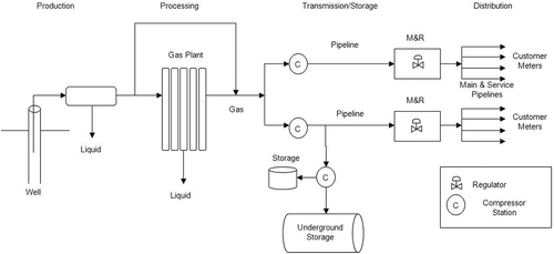
Natural gas production begins with withdrawal of raw gas from underground reservoirs. After reaching the surface, raw gas is treated and passed along for processing to remove liquids and other undesirable constituents (Figure 1). It should be noted that this study was done only on conventional natural gas, and not on unconventional natural gas (e.g., that produced from fracking). Equipment in the production sector includes wellheads, separators, dehydrators, compressors, pneumatic devices, and pipelines, while equipment in the processing sector includes dehydrators, compressors, pneumatic devices, and pipelines. Transmission of natural gas from production and processing (P&P) facilities to distribution pipelines is achieved with high-pressure, large-diameter pipelines. This sector equipment includes compressors, pipelines, meters, regulators, and pneumatic devices. Natural gas is then often stored to compensate for times of high and low demands. The storage sector equipment includes wellheads, compressors, dehydrators, pneumatic devices, and pipelines. The distribution sector receives high-pressure gas from transmission pipelines, reduces the pressure, and distributes the gas to customers. This sector equipment includes metering and regulating (M&R) stations, customer meters, pneumatic devices, and pipelines.

Figure 1. Process flow diagram of natural gas industry.

Sources of methane emissions in the natural gas industry can be categorized into combustion, vented, fugitive, and other (nonroutine) emissions (INGAA Foundation, 2005). Combustion, vented, and nonroutine emissions are intentional/controlled releases, while fugitive emissions are unintentional releases of natural gas from processes and equipment into the ambient air. Pressurized equipment has the potential to leak, and these leaks generally occur through equipment components such as valves, flanges, seals, open-ended lines (OELs), and pressure relief valves (PRVs). Fugitive emissions can also be from nonpoint evaporative sources such as wastewater treatment, pits, and surface impoundments (American Petroleum Institute [API], 2009). This study was focused only on fugitive emissions from pressurized equipment and its components.

There are 703 onshore natural gas production, 17 processing, and 10 storage facilities in California. Methane emissions from California’s oil and natural gas industry in year 2007 were 10,836, 24,880, and 73,551 metric tons/year (MT/yr) from combustion, vents, and fugitive sources, respectively; and the fugitive emissions accounted for 67% of the total (California Air Resources Board [CARB], 2011). Fugitive methane emissions were 10,022, 10,605, and 8,380 MT/yr from onshore production, processing, and storage facilities, respectively. Fugitive emissions by equipment type were 11,336, 2,032, and 170 MT/yr for dehydrators, wellheads, and separators, respectively (CARB, 2011).

Emission Factors

Over the past decade there has been a growing need to understand methane emissions from the natural gas system. The emission estimates are often derived by using emission factors (EFs) coupled with activity factors. A number of EFs and correlation equations have been generated for estimation of fugitive emissions from equipment leaks (U.S. Environmental Protection Agency [EPA], 1995; EPA/Gas Research Institute [GRI], 1996; API, 2004; Canadian Energy Partnership for Environmental Innovation [CEPEI], 2007). These EFs can be categorized into three levels: facility, equipment, and component (EPA, 1995; API, 2009). Using a facility-level EF to estimate methane emission is the simplest approach, requiring only information on type and capacity of a specific facility. The equipment-level EF approach is one level up and requires an accurate count of all major pieces of equipment. The component-level EFs can be further categorized into four groups, in order of increasing data requirements and increasing accuracy for emission estimates: average EF, screening ranges, correlation equation, and unit-specific correlation (EPA, 1995; API, 2004).

Use of component-level average EFs for emission estimate needs only the population data of components at a given facility, while the other three component-level EFs approaches require screening data from a leak detection and repair (LDAR) program (API, 2009). Screening data are collected by using a portable monitoring instrument to sample air from potential leak interfaces on individual equipment components. A screening value (SV) is a measure of the concentration of leaking compounds in the ambient air, typically in parts per million by volume (ppmV) by a portable instrument. The instrument typically has a lower limit (the detection limit) and a higher limit (the pegged SV). The screening-ranges approach divides the SVs into two or more ranges and an EF is assigned to each range. In older regulations, 10,000 ppmV was often used as the leak definition (EPA/GRI, 1996). The approach is also known as the “leak/no leak” approach, with the “leakers” having SVs ≥ 10,000 ppmV and “nonleakers” having SVs <10,000 ppmV. The correlation-equation approach uses both the SV of a leaking component and the established correlation equations between SVs and leak rates for emission estimate. Each correlation equation is specific to the component type. Using this approach the emission rate for each leaking component is calculated individually and the facility needs to keep track of the findings from the LDAR activities (API, 2009). The unit-specific correlation approach is similar, except the correlations are unit-specific and/or site-specific. This approach can be expensive and would seldom justify developing unit-specific correlations to support estimates for GHG emissions (API, 2004).

The Compendium of Greenhouse Gas Emission Estimation Methodologies for the Oil and Gas Industry developed by the American Petroleum Institute (API) is commonly used in preparation of methane emission inventory reports (API, 2009). Although the document is relatively new, the EFs contained in it were mainly from a 1996 report by the EPA and the Gas Research Institute (GRI) (EPA/GRI, 1996). Many of these EFs may not be applicable to California now due to differences in compliance requirements and in operation and maintenance practices. As an example, California Air Pollution Control Officers Association (CAPCOA) and the California Air Resources Board (CARB) revised some of the EFs of the 1999 EPA/GRI study (CAPCOA, 1999). While other EFs have been published (Chambers et al., 2006; CEPEI, 2007; Vorgang et al., 2009; Marcogaz-EuroGas, 2011), the 1996 EPA/GRI study remains the cornerstone for U.S. natural gas industry methane emission quantification (American Gas Association [AGA], 2008).

Objectives of this Study

The overall objective of this project was to develop current, reliable, and California-specific source EFs that can then be used to establish a more accurate methane emission inventory for the California natural gas system. The results from this project could also be used to support regulatory programs to achieve effective and efficient methane emission reductions from California’s natural gas system, consequently minimizing adverse environmental impacts. The goal of the project was to test as many systems and components in as many facilities as possible to obtain representative samples from all sectors of the California natural gas industry.

Experimental Approaches and Methods

Field test protocols and instruments

The test plan of this study was developed in coordination with CARB and followed its test protocol titled Draft Test Protocol—Detection and Quantification of Fugitive and Vented Methane, Carbon Dioxide, and Volatile Organic Compounds from Crude Oil and Natural Gas Facilities (CARB, 2009; CARB, 2010). According to the protocol, a screening device is first used to locate the presence of fugitive methane from a distance, followed by a detection device to locate the specific fugitive leak source. A bagging method or a third device is then used to quantify the leak rate. The required detection limits are ≤100 ppmV and ≤0.5 standard cubic feet per minute (scfm) for the detection device and the quantification device, respectively. The required ranges are at least 100 to 10,000 ppmV and 0.5 to 8.0 scfm for the detection device and the quantification device, respectively.

The type of screening devices used in this study was the Remote Methane Leak Detector (RMLD; Heath Consultants, Houston, TX), which uses a tunable diode laser absorption spectroscopy to identify presence of methane within a range of 100 feet (Heath, 2005). The detection devices used were two RKI Eagle (RKI Instruments, Union City, CA) units with a methane detection range of 0 to 50,000 ppmV. Each RKI Eagle unit was equipped with a Teflon tube from which the gas was drawn to the sensors (RKI Instruments, 2011). In this study, the tube was placed 1 cm around specific components until the largest concentration was found. The leak rate quantification devices used were two Bacharach Hi-Flow samplers (Heath Consultants, Houston, TX) with a quantification range of 0.01 and 8 scfm. A large 1.5-inch diameter pipe was used to vacuum methane through its sensors (Bacharach Inc., 2010). An antistatic bag was used to quantify the rate of a larger leak. All the instruments were calibrated according to manufacturers’ specifications at the beginning of each test day and at the end of each day. If any of the devices was found to be out of calibration at the end of the inspection, the data from that device would be regarded as inaccurate and would therefore be discarded. The event of data being deemed irrelevant due to an error in calibration at the end of the test day never occurred over the course of this study.

Types of equipment/components

Types of equipment surveyed in this study included wellheads, separators, dehydrators, piping segments, compressors, pneumatic devices, M&R stations, hatches, pumps, and customer meters. Nine types of equipment components were considered: flange, manual valve, OEL, PRV, regulator, seal, threaded connection, welded connection, and “others.” For the purpose of this study, an OEL is any line that is open to atmosphere including pipes or the open end of a valve. A PRV refers to a device that is used to prevent the over-pressurization of a piping system, vessel, or other system. A regulator is an automatic device that regulates the flow or pressure of a gas line. A seal refers to any mechanism used to contain liquid or gas within a line or vessel. The “others” category refers to other components not defined in the preceding terms.

Results and Discussion

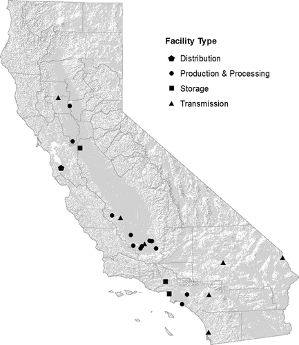
A total of 25 facilities were surveyed during 27 visits, and their locations are plotted in Figure 2. They include 12 facilities in the production and processing (P&P) sector, 3 facilities in the storage sector, 8 facilities in the transmission sector, and 2 facilities in the distribution sectors. Of these visits, 24 were scheduled and 3 were surprise visits accompanied by local air districts personnel. Most of the facilities were too large to survey in their entirety, so representative portions of each facility were surveyed. In addition, some equipment items (e.g., compressors, dehydrators, and separators) were large and some of their components could not be readily accessed for screening. Surveyed equipment included wellheads (172), separators (131), dehydrators (17), piping segments (145), compressors (66), pneumatic devices (374), M&R stations (19), hatches (34), pumps (2), and customer meters (12). In total, 92,157 components were surveyed, and the breakdown of the components surveyed can be found in Table 1.

Table 1. Counts of components surveyed and percentages of leaking ones

	Counts of component surveyed	Counts of component with SV >100 ppmV	Percentage of components with SV >100 ppmV
Flanges	10,101	56	0.55%
Manual valves	10,765	49	0.46%
OELs	384	26	6.77%
Others	138	44	31.9%
PRVs	358	6	1.68%
Regulators	930	13	1.40%
Seals	146	61	41.8%
Threaded connections	57,601	123	0.21%
Welded connections	12,274	0	0%

Figure 2. Locations of facilities surveyed.

Out of 92,157 equipment components surveyed, 380 locations (i.e., 0.41%) showed positive SV readings, 2 of which had concentrations less than 100 ppmV. These two locations were excluded from further analysis because they might not be picked up by devices that comply with CARB’s requirement on detection limit of 100 ppmV. Consequently, the other 378 locations were considered as leaking sources in this study. Table 1 also tabulates the counts and percentages of leaking sources.

Two Hi-Flow samplers were used to quantify emissions from the leaking sources. These samplers quantified the emission rate directly by taking both concentration and sample flow rate measurements. Using Hi-Flow samplers is much faster than using an enclosure method (i.e., the bagging approach), which is more time-consuming and labor-intensive. However, the high dilution rate used by the samplers would lead to lower concentrations (i.e., lower resolution) for small leaks that might become nondetects by the Hi-Flow samplers (EPA/GRI, 1996).

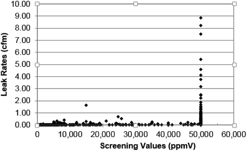
Figure 3 plots leak rates versus SVs of all 378 leaking components. (The maximum detection limit of the device used was 50,000 ppmV. Data with an SV ≥50,000 ppmV were plotted as 50,000 ppmV in this figure.) As shown, the SVs spanned several orders of magnitude and the leak rates were highly variable. The high variability in measured leakage rates was also found in the EPA/GRI (1996) study; as an example, the leak rates of connectors varied more than four orders of magnitude for similar SVs (Figure 3–11 of Volume 8 of the 1996 EPA/GRI report). Many of the leaking components have high SVs, but their leak rates are below the detection limit. This implies a poor correlation between the measured leak rates and the measured SVs. One plausible reason for the poor correlation is that an SV represents the ambient concentration in the vicinity of the leak, while the mass leak rate depends on factors such as size of the imperfection and the internal pressure.

Figure 3. Leak rates versus SVs for all leaking components.

Screening-ranges EFs

The first part of the data analysis was to develop screening-ranges EFs. The measured SVs were first split into two groups: 0 to 9,999 and ≥ 10,000 ppmV. The value 10,000 ppmV was chosen as the boundary for these two groups is because 10,000 ppmV was often used as the leak definition (EPA, 1995; EPA/GRI, 1996; API, 2004). Leaking sources with registered SV readings but with corresponding leaking rates below the detection limit were assigned a leak rate of 0.005 cfm, which is half of the detection limit.

Table 2 tabulates some statistics of the leak rates (count, minimum, maximum, median, arithmetic average, and geometric mean) for two groups of SVs (<10,000 and ≥ 10,000 ppmV). The majority of the leaking components (261/378 = 69%) have an SV ≥ 10,000 ppmV. The leak rates of the <10,000 ppmV group range from 0.005 (below the detection limit of 0.01 cfm) to 0.41 cfm, while those of the ≥ 10,000 ppmV group range from 0.005 to 8.85 cfm. For both ranges of the SVs, the arithmetic averages of the leak rates are larger than the corresponding median and geometric mean (geomean) values.

Table 2. Leak rates versus SVs in two ranges (all components)

		Leak rate (cfm)
SV (ppmV)	Count	Minimum	Maximum	Median	Average	Geomean
100–9,999	117	0.005	0.410	0.005	0.024	0.0079
≥10,000	261	0.005	8.850	0.040	0.378	0.0317
Total	378	0.005	8.850	0.010	0.269	0.0291

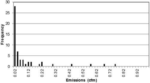
The histograms of leak rates were then plotted for each type of the components surveyed. Figure 4 shows the leak-rate histogram of flanges as an example. The majority of leakage rates were within the range of <0.01 to 0.02 cfm. For emission rates greater than 0.02 cfm, the frequency at which the leakages occurred decreased as the emission rate increased. The histograms of other types of components surveyed appeared to have the same trend.

Figure 4. Leak-rate histograms of flanges.

The histograms were then further evaluated for probability distribution. The Weibull probability distribution function (PDF) was found to fit the histograms well. A cumulative distribution function (CDF) calculates the probability that a leakage rate will be located between 0 and a random leakage rate, x. The Weibull CDF can be expressed as

(1)

The cumulative probability for leak rates from 0 cfm to infinite will be equal to unity. Similar to the PDF, the CDF is dependent on the shape parameter, k, and the scale parameter, λ. The Weibull CDF was used in this study to determine if the geometric mean or the arithmetic average is a better indicator as the mean for each range of the leakage rates. The closer the cumulative probability is to 50%, more evenly distributed the range becomes. The results indicate that using the geometric mean yields a cumulative probability typically closer to 50% than that using the arithmetic mean for the majority of the component types and for different SV groups. It implies that the geometric mean is a better indicator than the arithmetic mean as the mean for each group of leakage rates found in this study. In addition, the measured leak rates for a given type of component often spanned widely in this study. One could use the arithmetic, median, or geometric mean as the mean of a data set. However, using arithmetic means for the data sets generated in this study, the average values would probably be skewed by the large values or the outliers. Using the median may not take the large values into consideration. Consequently, the geometric means, instead of arithmetic means, were used to derive the EFs in this study.

The portable detection devices used in this study have a maximum detection limit of 50,000 ppmV. The data sets were further divided into four ranges: 0 to 999, 1,000 to 9,999, 10,000 to 49,999, and ≥50,000 ppmV. The first group, “0–999 ppmV,” was designated as such because all the measured leak rates in this group were below the detection limit of 0.01 cfm. The second group, “1,000-9,999 ppmV,” reflects the typical leak definition, 10,000 ppmV, in earlier regulations. The third group (10,000–49,999 ppmV) and the last group (≥50,000 ppmV) were chosen to take advantage of the maximum detection value (50,000 ppmV) of the portable detection devices used in this study.

The screening-ranges EFs for flanges, manual valves, OELs, “others,” seals, and threaded connections are summarized in Table 3 (PRVs and regulators were not included in this part of data analysis because of small sample sizes of leaking sources and because there were no leaks found in any welded connection screened). The geomeans of the leak rates increase with SVs.

Table 3. Leak rates (cfm) versus SVs in four ranges

SV (ppmV)	100–999	1,000–9,999	10,000–49,999	≥ 50,000
Flanges	0.0050 (2)*	0.0067 (20)	0.0293 (17)	0.0747 (17)
Manual valves	0.0050 (1)	0.0050 (17)	0.0136 (13)	0.0197 (18)
OELs	—	0.0050 (3)	0.0050 (5)	0.2874 (18)
Others	—	0.0310 (8)	0.0691 (10)	0.1157 (26)
Seals	0.0050 (8)	0.0527 (5)	0.1217 (3)	0.3907 (45)
Threaded connections	0.0050 (5)	0.0068 (38)	0.0143 (41)	0.0168 (39)

*Counts of leaking components.

Table 4 tabulates the ranges of component leak rates along with the pegged EFs for ≥ 10,000 and ≥ 50,000 ppmV. The pegged emission rate is the mass emission rate with an SV that is above the maximum detection limit of a portable screening device. As shown, the pegged EFs for ≥10,000 and ≥ 50,000 ppmV are similar for manual valves, “others,” seals, and threaded connections, while the pegged EFs of ≥ 50,000 ppmV are approximately twice as larger as those of ≥ 10,000 ppmV for flanges and OELs.

Table 4. Ranges of component leak rates and pegged EFs

	Leak rate (cfm)
	Count	Min	Max	≥ 10,000 ppmV	≥ 50,000 ppmV
Flanges	56	0.005	0.750	0.0468	0.0747
Manual valves	49	0.005	0.160	0.0169	0.0197
OELs	26	0.005	8.850	0.1191	0.2874
Others	44	0.005	3.180	0.1002	0.1157
Seals	61	0.005	8.220	0.3632	0.3907
Threaded connections	123	0.005	0.430	0.0155	0.0168

In 1999, CAPCOA and CARB revised some of the EFs reported in the 1996 EPA/GRI study (CAPCOA, 1999). Table 5 compares the pegged EFs of this study with those of the two studies. Similar to the findings in this study, the EFs of a larger pegged value (100,000 ppmV) are similar to or twice as large as the corresponding values of a much smaller pegged value (10,000 ppmV) in the 1996 EPA/GRI study. Comparing the EFs with a pegged value of 10,000 ppmV, flanges and threaded connections surveyed in this study have smaller EFs than those in the 1996 EPA/GRI and 1999 CAPCOA studies; they are 2.81 versus 4.50 vs. 3.22 lb/day, and 0.93 versus 1.48 vs. 1.37 lb/day, respectively. On the other hand, those of OELs and “others” in this study are higher (7.14 vs. 1.59 vs. 2.90 lb/day and 6.01 vs. 3.86 vs. 0.73 lb/day). That of manual valves in this study falls between those of the two studies (1.01 vs. 3.39 vs. 0.73 lb/day). The data for seals are not comparable because the seals in this study were mainly compressor seals while those in the EPA/GRI study were pump seals. The differences in the units (lb methane/day for this study vs. lb total hydrocarbon [THC])/d for those two studies) should be noted. The COPCOA’s EFs were derived for oil and gas production and for gas/light liquid service. These EFs are for the total organic compound emission rates (including those that are not volatile organic compounds [VOCs], such as methane and ethane). On the other hand, this study was for the natural gas industry only. For a fair comparison between these two data sets, a methane/THC ratio should have been used. However, applying a fixed methane/THC ratio would not be practical since the ratio would be site specific and dependent on the composition of the natural gas.

Table 5. Comparison of pegged EFs

	CEC (2012)			EPA/GRI (1996)			CAPCOA (1999)
	≥ 10,000 ppmV	≥ 50,000 ppmV		≥ 10,000 ppmV	≥ 100,000 ppmV		≥ 10,000 ppmV
	(lb methane/day)*			(lb THC/day)			(lb THC/d)
Flanges	2.81	4.48		4.50	4.44		3.22
Manual valves	1.01	1.18		3.39	7.41		0.73
OELs	7.14	17.24		1.59	4.18		2.90
Others	6.01	6.94		3.86	5.82		0.73
Seals	21.79	23.43		3.92	8.47		N/A
Threaded connections	0.93	1.01		1.48	1.59		1.37

*1 cubic feet methane/minute = 1.136 kg methane/hr = 9.906 tonne methane/yr = 59.98 lb methane/day.

Component-level correlation-equation EFs

The component-level correlation-equation approach is often used to estimate an emission rate from a leaking component using a corresponding SV, especially for facilities with LDAR programs in place. The correlation equations are commonly expressed as

(2)

where LR_methane is the methane leak rate (e.g., in cfm), a and b are constants developed from the correlation fitting, and SV is the screening value (e.g., in ppmV).

In this study the correlation equations were derived for the entire range of SVs (100–49,999 ppmV) for all types of components surveyed with decent sample sizes. Figure 5 shows the correlation equation of flanges as an example.

Figure 5. Correlation equation for flanges.

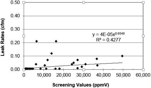
The correlation equations for flanges, manual valves, others, seals, and threaded connections along with their R² values are tabulated in Table 6 for SVs ranging from 100 to 49,999 ppmV. Although there were leaking OELs with SVs < 50,000 ppmV, the corresponding leak rates were all below the detection limit of 0.01 cfm. Consequently, no correlation equation was derived for OELs. As shown, the values of the correlation coefficient (R) for flanges (0.65) and for seals (0.67) are decent, while those for manual valves (0.35) and threaded connections (0.33) are small.

Table 6. Correlation equations for leak rates (cfm) of different types of components (SV from 100 to 49,999 ppmV)

	Correlation equation	R^2
Flanges	LRmethane = 0.00004 × (SV)^0.6549	0.4277
Manual valves	LRmethane = 0.0006 × (SV)^0.2811	0.1204
Others	LRmethane = 0.0003 × (SV)^0.5353	0.1008
Seals	LRmethane = 0.0001 × (SV)^0.6816	0.4504
Threaded connections	LRmethane = 0.0006 × (SV)^0.3031	0.1150

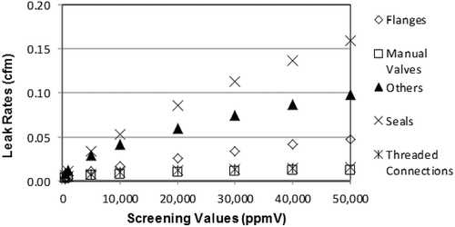
Figure 6 plots the leak rates versus SVs using the correlation equations derived in this study (Table 6). As shown, the calculated leak rates for the same SV are different for different component types. For a specific SV, the calculated leak rates will be in the following decreasing order: seals, “others,” flanges, threaded connections, and manual valves.

Figure 6. Leak rates vs. SVs using the correlation equations.

Table 7 tabulates the correlation equations for leak rates (kg/hr) of the 1996 EPA/GRI study, the 1999 CAPCOA study and this study. The correlation equations for the EPA/GRI and CAPCOA studies were similar. The calculated leak rates using the correlation equations of this study would be several times higher than those using the EPA/GRI or CAPCOA correlation equations. The differences may be partly attributed to the poor correlation between the leak rates and SVs in this study and the larger detection limit of the Hi-Flow samplers. In addition, the correlation equations in this study only used data from the natural gas industry. Those of the EPA/GRI and the CAPCOA studies were based on data from petroleum refineries, marketing terminals, and oil and gas production and were combined for all service types (i.e., gas, light liquid, heavy liquid). It should be noted that the EPA issued final air rules for the oil and natural gas industry on April 17, 2012, with the goals of these rules being the reduction of emissions from this industry (EPA, 2012).

Table 7. Comparison of correlation equations for leak rates (kg/hr)

	EPA/GRI (1996)	CAPCOA (1999)	CEC (2012)
Connectors	(1.52 × 10^−6) × (SV)^0.735	(1.53 × 10^−6) × (SV)^0.736	(6.78 × 10^−4) × (SV)^0.3031
Flanges	(4.44 × 10^−6) × (SV)^0.703	(4.53 × 10^−6) × (SV)^0.706	(4.52 × 10^−5) × (SV)^0.6549
OELs	(2.16 × 10^−6) × (SV)^0.704	(1.90 × 10^−6) × (SV)^0.724	N/A
Pump seals	(4.82 × 10^−5) × (SV)^0.610	(5.07 × 10^−5) × (SV)^0.622	N/A
Valves	(2.29 × 10^−6) × (SV)^0.746	(2.27 × 10^−6) × (SV)^0.747	(6.78 × 10^−4) × (SV)^0.2811
Others	(1.32 × 10^−5) × (SV)^0.589	(8.69 × 10^−6) × (SV)^0.642	(3.39 × 10^−4) × (SV)^0.5353

Component-level and equipment-level average emission factors

The field data were also used to generate component-level average EFs. These EFs were then used to develop equipment-level average EFs when appropriate. This section first presents the approaches used to derive EFs of wellhead components and then EFs of wellhead as a system. The component-level average EFs for separators, dehydrators, piping segments, compressors, and M&R stations are then presented.

Wellheads

A wellhead is the uppermost part of a natural gas well located at production or storage facilities. For each wellhead surveyed, all components were screened from the ground up. The numbers of wellheads surveyed were 128 and 44 in the production and the storage sectors, respectively. Table 8 tabulates ranges and average counts of components per wellhead for both sectors. As shown, wellheads in the storage sector on average have more component counts per wellhead than those in the production sector.

Table 8. Component counts per wellhead

	Production		Storage
	Range	Average	Range	Average
Flanges	0–23	5.8	3–44	20.4
Manual valves	4–20	7.5	1–41	24.0
OELs	0–0	0.0	0–12	0.8
Others	0–2	0.5	0–1	0.0
PRVs	0–2	0.2	0–2	0.3
Regulators	0–2	0.2	0–7	1.3
Seals	0–2	0.8	0–0	0
Threaded connections	3–111	27.5	5–212	102.9
Welded connections	0–14	2.5	0–36	9.1

Table 9 shows the leaking percentage of each type of wellhead component surveyed. Table 10 tabulates the ranges and geomeans of the component leak rates by industry sector.

Table 9. Leaking percentages of components (wellhead).

	Production		Storage
	Leaking/total	%	Leaking/total	%
Flanges	5/742	0.67%	0/899	0%
Manual valves	2/958	0.21%	25/1057	2.37%
OELs	0/0	—	8/133	6.02%
Others	0/70	0%	1/1	100%
PRVs	0/23	0%	0/14	0%
Regulators	0/24	0%	0/59	0%
Seals	9/107	8.41%	0/0	—
Threaded connections	7/3515	0.20%	14/4529	0.31%
Welded connections	0/324	0%	0/400	0%

Table 10. Mean leak rates (cfm) of leaking components (wellheads)

	Production		Storage
	Range of leakages	Geomean	Range of leakages	Geomean
Flanges	0.005–0.10	3.14E-04	—	—
Manual valves	0.005–0.20	2.83E-02	0.005–0.35	3.88E-02
OELs	—	—	0.02–1.35	1.75E-02
Others	—	—	0.22–0.22	2.20E-01
PRVs	—	—	—	—
Regulators	—	—	—	—
Seals	0.005–0.08	7.05E-03	—	—
Threaded connections	0.005–0.16	3.14E-02	0.005–1.25	4.16E-02
Welded connections	—	—	—	—

Table 11 shows the component-level average EFs which were calculated by using the leaking percentages (Table 9) and the mean leak rates (Table 10). For wellheads in the sector, the component-level average EF is the largest for seals at 5.93 × 10⁻⁴ cfm, followed by 2.12 × 10⁻⁴ cfm for flanges, 6.25 × 10⁻⁵ cfm for threaded connections, and 5.90 × 10⁻⁵ cfm for manual valves. For the storage sector, the largest is 2.20 × 10⁻¹ cfm for “others,” followed by 1.05 × 10⁻³ cfm for OELs, 9.18 × 10⁻⁴ cfm for manual valves, and 1.28 × 10⁻⁴ cfm for threaded connections (Table 11). The EFs in Table 11 are also given in units of tonnes methane per year per component to facilitate a comparison with the benchmark EFs reported in the 1996 EPA/GRI study. The conversion factor from cubic feet per minute (cfm) to tonnes methane per year is equal to 9.906.

Table 11. Component-level EFs by industry sector (wellheads)

	Production		Storage
	cfm CH4/component	tonne CH4/yr/component	cfm CH4/component	tonne CH4/yr/component
Flanges	2.12E-04	2.10E-03	—	—
Manual valves	5.90E-05	5.85E-04	9.18E-04	9.09E-03
OELs	—	—	1.05E-03	1.04E-02
Others	—	—	2.20E-01	2.18E-00
PRVs	—	—	—	—
Regulators	—	—	—	—
Seals	5.93E-04	5.87E-03	—	—
Threaded connections	6.25E-05	6.20E-04	1.28E-04	1.27E-03
Welded connections	—	—	—	—

Table 12 compares the component-level average EFs derived in this study with those from the 1996 EPA/GRI study. Not all the components have EF values from both studies, but the values of the corresponding EFs are relatively comparable. The EFs of this study are all smaller than those of the EPA/GRI study, except the EF of OELs in the storage sector. The smaller EF values from this study might be partially attributable to the employment of the LDAR program by most, if not all, of the facilities surveyed.

Table 12. Comparison of component-level EFs (tonnes methane/yr/component)—Wellheads

	Production		Storage
	(CEC, 2012)	(EPA/GRI, 1996)	(CEC, 2012)	(EPA/GRI, 1996)
Flanges	2.10E-03	—	—	—
Manual valves	5.85E-04	1.57E-02	9.09E-03	1.73E-02
OELs	—	4.05E-03	1.04E-02	4.47E-03
Others	—	—	2.18E-00	—
PRVs	—	—	—	2.76E-02
Regulators	—	—	—	—
Seals	5.87E-03	—	—	—
Threaded connections	6.20E-04	2.15E-03	1.27E-03	2.36E-03
Welded connections	—	—	—	—

To derive a fugitive EF for a wellhead as a whole, the EF of each component was first multiplied by the average number of that component per wellhead. The multiplication products of all components were then summed to become the average EF of a wellhead. For comparison, the component count data and EFs of the 1996 EPA/GRI study were also used to derive the EF values of wellheads. As shown in Table 13, the wellhead EFs of this study are comparable to the corresponding ones of the EPA/GRI, but smaller.

Table 13. Comparison of equipment-level EFs (Wellheads)

	(tonnes methane/yr/wellhead)
	Production	Storage
CEC (2012)	3.83E-02	3.49E-01
EPA/GRI (1996)	2.54E-01	7.88E-01

Separators

A separator is a piece of equipment utilized to remove condensate and oil from natural gas. Many separators can be very large and therefore some sections are inaccessible without the use of a manlift. All accessible components of each separator surveyed in this study were screened. The numbers of separators surveyed were 115, 14, and 2 in the P&P, storage, and transmission sectors, respectively.

Table 14 tabulates the component-level average EFs derived in this study and those from the 1996 EPA/GRI study. Both studies have average EFs for manual valves, OELs, PRVs, and threaded connections. The EFs of this study are smaller than the corresponding values of the EPA/GRI study.

Table 14. Comparison of component-level emission factors (tonnes methane/yr/component)—Separators

	P&P		Storage
	(CEC, 2012)	(EPA/GRI, 1996)	(CEC, 2012)
Flanges	1.55E-04	—	—
Manual valves	2.61E-04	1.57E-02	—
OELs	—	4.05E-03	2.68E-03
Others	1.98E-01	—	5.83E-03
PRVs	2.15E-03	2.51E-02	—
Regulators	2.71E-03	—	—
Seals	—	—	—
Threaded connections	6.02E-05	2.15E-03	5.75E-05

Dehydrators

A dehydrator is a unit that is used to remove water from natural gas. A dehydrator is typically composed of a contactor and a reboiler. These devices have large tanks that process the natural gas. Dehydrators can be very large and therefore some sections are inaccessible without the use of a manlift. All accessible components of each dehydrator tested in this study were screened. The research team visited 4 facilities having dehydrators, and 17 dehydrators were screened (8 in the P&P and 9 in the storage sectors).

Table 15 tabulates the component-level average EFs derived in this study and those from the 1996 EPA/GRI study. Both studies have average EFs for threaded connections and the EF of this study is smaller than the corresponding value from the EPA/GRI study.

Table 15. Comparison of component-level EFs (tonnes methane/yr/component)—Dehydrators

	P & P
	(CEC, 2012)	(EPA/GRI, 1996)
Flanges	1.58E-03	—
Manual valves	—	1.57E-02
OELs	—	4.05E-03
Others	—	—
PRVs	—	2.51E-02
Regulators	6.28E-02	—
Seals	—	—
Threaded connections	2.44E-04	2.15E-03

Piping segments

A piping segment is any portion of piping between equipment systems. It transmits the gas from one system to another or off site. Most screened piping segments were between two systems that were readily accessed. The research team visited 15 facilities to survey 145 piping segments in total (64 in P&P, 21 in the storage, 28 in the transmission, and 32 in the distribution sectors).

Table 16 shows the component-level average EFs of the piping segments by industry sectors. Across the industry sectors, the EFs of flanges, manual valves, and threaded connections are relatively comparable. On the other hand, the EF for OELs in the transmission sector is larger than those of the P&P and storage sectors, while the EF of regulators in the storage sector is larger than that in the P&P sector. The larger values are mainly due to a small number of large leaks found in surveying.

Table 16. Component average emission factor by industry segment (piping segments)

	tonnes methane/yr/ component
	P&P	Storage	Transmission	Distribution	(EPA/GRI, 1996)
Flanges	6.57E-05	7.23E-04	1.10E-04	—	—
Manual valves	2.35E-04	2.12E-04	1.43E-03	1.47E-03	1,57E-02
OELs	7.08E-03	1.09E-03	1.50E+01	—	4.05E-03
Others	4.90E-02	—	—	—	—
PRVs	—	2.43E-01	—	—	2.52E-02
Regulators	4.30E-03	4.59E-01	—	—	—
Seals	—	—	—	—	—
Threaded connections	6.63E-04	6.45E-04	6.36E-04	2.16E-04	2.15E-03
Welded connections	—	—	—	—	-

The last column lists the EFs of the production sector in the 1996 EPA/GRI study for comparison. As shown, the EFs of manual valves and threaded connections of this study are smaller than the corresponding ones of the EPA/GRI study; those of OELs of the P&P and transmission sectors are larger while that of the storage sector is smaller.

Compressors—reciprocating compressors

Compressors are commonly used throughout the natural gas industry to pressurize gas. Each compressor is classified according to the mechanism it utilizes to compress the natural gas. A reciprocating compressor refers to a compressor that uses pistons to compress and pressurize the natural gas and then discharge it. All accessible components of each reciprocating compressor surveyed in this study were screened. The research team visited 9 facilities to survey 51 reciprocating compressors (36 in the P&P, 7 in the storage, 8 in the transmission sectors). Table 17 tabulates the component-level average EFs derived in this study.

Table 17. Comparison of component-level emission factors (tonnes methane/yr/component)—Reciprocating compressors

	P & P	Storage	Transmission
Flanges	9.49E-03	—	4.58E-02
Manual valves	1.49E-04	1.62E-03	2.71E-04
OELs	6.63E-01	—	—
Others	—	—	—
PRVs	—	—	—
Regulators	1.04E-03	—	—
Seals	—	—	1.51E-01
Threaded connections	2.88E-04	—	7.42E-04
Welded connections	—	—	—

Compressors—centrifugal compressors

A centrifugal compressor compresses gas by accelerating it using a turbine and then converting this velocity into compression. All accessible components of each centrifugal compressor surveyed in this study were screened. The research team visited three facilities having centrifugal compressors, at which nine centrifugal compressors in total were screened (four in the P&P, three in the storage, and two in the transmission sectors). Table 18 tabulates the component average EFs derived in this study.

Table 18. Comparison of component–level emission factors (tonnes methane/yr/component)—Centrifugal compressors

	P & P	Storage	Transmission
Flange	—	—	1.21E-02
Manual valve	—	8.04E-03	—
OELs	—	—	—
Other	—	—	—
PRVs	—	—	—
Regulators	—	—	—
Seal	—	—	5.94E-01
Threaded connection	9.33-05	4.14E-04	—
Welded connections	—	—	—

M&R Stations

Metering and regulating (M&R) stations are typically designed to provide a constant output from the facility with constant pressure and other characteristics to the downstream facility. M&R stations are usually composed of many piping segments without much complex equipment; therefore, all segments were screened, excluding any compressed air systems to control flow.

The research team visited two facilities. In total, 19 M&R stations were screened (4 in the transmission and 15 in the distribution sectors). Table 19 tabulates the component average EFs derived in this study.

Table 19. Component average EFs by industry sector—M&R station

	Distribution
	(tonnes methane/yr/component)
Flanges	5.93E-04
Manual valves	2.12E-04
OELs	—
Others	—
PRVs	—
Regulators	—
Seals	—
Threaded connections	—
Welded connections	—

Conclusion

Concluding remarks of this study are as follows:

1. Twenty-five California natural gas facilities from all five sectors (production, processing, storage, transmission, and distribution) were surveyed to quantify the screening values (SVs) and fugitive emission rates from leaking equipment components. The systems surveyed include wellheads, separators, dehydrators, piping segments, compressors, pneumatic devices, metering and regulating stations, hatches, pumps, and customer meters, while the components studied were flanges, manual valves, open-ended lines (OELs), “others,” pressure relief valves (PRVs), regulators, seals, threaded connections, and welded connections.

2. Hi-Flow samplers were used to quantify fugitive emission rates. Using Hi-Flow samplers is much faster than the bagging approach, but the higher dilution rate used by the Hi-Flow samplers would lead to lower concentrations (i.e., lower resolution) for small leaks that may become non-detects.

3. For a given SV range, the measured leak rates might span several orders of magnitude. Many of the leaking components had high SVs, but their leak rates were below the detection limit of the flow rate device. This implies a poor correlation between the leak rates and the SVs.

4. All the component leakage rate histograms appear to have the same trend. The majority of leakage rates were within the range of <0.01 to 0.02 cubic feet per minute (cfm). The frequency at which the leakages occurred decreased as the emission rate increased.

5. The Weibull probability distribution function (PDF) was found to fit the leakage rate histograms well. Using the cumulative distribution function (CDF), it was found that the geometric mean is a better indicator than the arithmetic average as the mean for each group of leakage rates found.

6. Pegged emission factors (EFs) for SVs of ≥10,000 ppmV and of ≥50,000 ppmV were derived. For most component types, the two values are relatively similar. However, the pegged EFs for seals and OELs are much higher than those of flanges, manual valves, and threaded connections.

7. The correlation equations between the leak rates and SVs were derived for several components. The values of the correlation coefficient (R) for flanges (0.65) and for seals (0.67) are decent, while those for manual valves (0.35) and threaded connections (0.33) are small.

8. Component-level average EFs for different component types were also derived. The EFs are often smaller than the corresponding ones in the 1996 EPA/GRI study.

Acknowledgments

The research team expresses its gratitude toward professionals at CEC (especially Guido Franco, the Commission Contract Manager) and CARB (especially Joe Fischer and James Nyarady), as well as the corporate and field professionals of the facilities that we have surveyed, for their great guidance and helpfulness.

Funding

This study was funded by the California Energy Commission under its Public Interest Energy Research (PIER) Program (agreement number 500-09-007).

Additional information

Funding

This study was funded by the California Energy Commission under its Public Interest Energy Research (PIER) Program (agreement number 500-09-007).

Notes on contributors

Jeff Kuo

Jeff Kuo is a professor at the Department of Civil and Environmental Engineering, California State University, Fullerton (CSUF).

Travis C. Hicks

Travis C. Hicks, Brian Drake, and Tat Fu Chan were graduate students at CSUF when the study was conducted.

Brian Drake

Travis C. Hicks, Brian Drake, and Tat Fu Chan were graduate students at CSUF when the study was conducted.

Tat Fu Chan

Travis C. Hicks, Brian Drake, and Tat Fu Chan were graduate students at CSUF when the study was conducted.

References

- American Gas Association. 2008. Greenhouse gas emissions estimation methodologies, procedures, and guidelines for the natural gas distribution sector. Report prepared by Innovative Environmental Solutions, Inc., for American Gas Association. http://s3.amazonaws.com/zanran_storage/www.aga.org/ContentPages/18068841.pdf
- American Petroleum Institute. 2004. Compendium of greenhouse gas emissions methodologies for the oil and gas industry. American Petroleum Institute, February. http://www.wrapair.org/ClimateChange/GHGProtocol/docs/2004-02_API_COMPENDIUM_of_GHG_Emission_Methodologies_from_O&G.pdf
- American Petroleum Institute. 2009. Compendium of greenhouse gas emissions methodologies for the oil and gas industry. American Petroleum Institute, August. http://www.api.org/~/media/Files/EHS/climate-change/2009_GHG_COMPENDIUM.ashx
- Bacharach, Inc. 2010. Operating Manual—Hi-Flow Sampler. New Kensington, PA: Bacharach, Inc.
- California Air Resources Board. 2009. Draft test protocol: Detection and quantification of fugitive and vented methane, carbon dioxide, and volatile organic compounds from crude oil and natural gas facilities. California Air Resources Board, November.
- California Air Resources Board. 2010. Draft test protocol: Detection and quantification of fugitive and vented methane, carbon dioxide, and volatile organic compounds from crude oil and natural gas facilities. California Air Resources Board, December (an updated version of 2009). http://www.arb.ca.gov/cc/oil-gas/fugitive_vented_protocol_dec29.pdf
- California Air Resources Board. 2011. 2007 Oil and gas industry survey results—Draft report. California Air Resources Board, August. http://www.arb.ca.gov/cc/oil-gas/finalreport.pdf
- Canadian Energy Partnership for Environmental Innovation. 2007. Methodology Manual—Estimation of Air Emissions from the Canadian Natural Gas Transmission, Storage and Distribution System. Prepared by Clearstone Engineering Ltd.
- California Air Pollution Control Officers Association. 1999. California implementation guidelines for estimating mass emissions of fugitive hydrocarbon leaks at petroleum facilities. Prepared by the California Air Pollution Control Officers Association Engineering Managers Committee and the California Air Resources Board Staff, February. http://www.arb.ca.gov/fugitive/impl_doc.pdf
- Chambers, A. K., M. Strosher, T. Wootton, J. Moncrieff, and P. McCready. 2006. DIAL measurements of fugitive emissions from natural gas plants and the comparison with emission factor estimates. http://www.epa.gov/ttnchie1/conference/ei15/session14/chambers.pdf.
- Choate, A., R. Kantamaneni, D. Lieberman, P. Mathis, B. Moore, D. Pape, L. Pederson, M. Van Pelt, and J. Venezia. 2005. Emission reduction opportunities for non-CO2 greenhouse gases in California. PIER Energy-Related Environmental Research California Energy Commission, CEC-500-2005-121. http://www.energy.ca.gov/2005publications/CEC-500-2005-121/CEC-500-2005-121.PDF
- Energy Information Administration. 2009. Emissions of Greenhouse Gases in the United States. Report prepared by U.S. Department of Energy, DOE/EIA-0573(2009). http://www.eia.gov/environment/emissions/ghg_report/pdf/0573(2009).pdf
- Heath Consultants, Inc. 2005. RMLD Remote Methane Leak Detector User’s Manual. Heath Consultants, Inc. http://heathus.com/wp-content/uploads/101296-0-RMLD-IS-Manual-Rev-J.pdf
- INGAA Foundation, Inc. 2005. Greenhouse gas emission estimation guidelines for natural gas transmission and storage. Report prepared by Innovative Environmental Solutions, Inc., for Interstate Natural Gas Association of America, Revision 2, September 28. http://www.ingaa.org/File.aspx?id=5485
- Marcogaz-EuroGas. 2011. Reduction of methane emissions in the European gas industry—Practices and technologies. Report by Macrogaz and Eurogas, JG-ENV-08-11, Groningen, The Netherlands.
- RKI Instruments. 2011. Instruction Manual, Eagle Series, Portable Multi-Gas Detector. RKI Instruments, Inc. http://www.rkiinstruments.com/pdf/meagle.pdf
- U.S. Environmental Protection Agency. 1995. Protocol for equipment leak emission estimates. EPA-453/R-95-017. U.S. EPA. http://www.epa.gov/ttnchie1/efdocs/equiplks.pdf
- U.S. Environmental Protection Agency. 2012. Oil and natural gas sector: New source performance standards and national emission standards for hazardous air pollutants reviews; Final rule. http://www.epa.gov/airquality/oilandgas/actions.html.
- U.S. Environmental Protection Agency/Gas Research Institute. 1996. Methane emissions from the natural gas industry. Prepared by Gas Research Institute (GRI), EPA/600/R-96/080, U.S. EPA. http://www.epa.gov/methane/gasstar/documents/emissions_report/3_generalmeth.pdf
- Vorgang, J., A. Riva, A. Cigni, and D. Hec. 2009. Reduction of methane emissions in the EU natural gas industry, http://www.igu.org/html/wgc2009/papers/docs/wgcFinal00187.pdf.