Physicochemical factors and sources of particulate matter at residential urban environment in Kuala Lumpur

Abstract

Long-term measurements (2004–2011) of PM₁₀ (particulate matter with an aerodynamic diameter <10 μm) and trace gases (carbon monoxide [CO], ozone [O₃], nitrogen oxide [NO], oxides of nitrogen [NO_x], nitrogen dioxide [NO₂], sulfur dioxide [SO₂], methane [CH₄], nonmethane hydrocarbon [NMHC]) have been conducted to study the effect of physicochemical factors on the PM₁₀ concentration. In addition, this study includes source apportionment of PM₁₀ in Kuala Lumpur urban environment. An advanced principal component analysis (PCA) technique coupled with absolute principal component scores (APCS) and multiple linear regression (MLR) has been applied. The average annual concentration of PM₁₀ for 8 yr is 51.3 ± 25.8 μg m⁻³, which exceeds the Recommended Malaysian Air Quality Guideline (RMAQG) and international guideline values. Detail analysis shows the dependency of PM₁₀ on the linear changes of the motor vehicles in use and the amount of biomass burning, particularly from Sumatra, Indonesia, during southwesterly monsoon. The main sources of PM₁₀ identified by PCA-APCS-MLR are traffic combustion (28%), ozone coupled with meteorological factors (20%), and windblown particles (1%). However, the apportionment procedure left 28.0 μg m⁻³, that is, 51% of PM₁₀ undetermined.

Implications: Air quality is always a top concern around the globe. Especially in the South Asian regions, measures are not yet sufficient; as revealed in our studies, the concentrations of particulate matters exceed the tolerable limits. Long-term data analysis and characterization of particular matters and their sources will aid the policy makers and the concerned authority to adapt measures and policies according to the circumstances. Additionally, similar intensive studies will give insight about future implications of air quality management.

Introduction

Atmospheric aerosols emitted from anthropogenic and natural sources play a vital role in the various atmospheric processes. Atmospheric aerosols affect the formation of cloud droplets, decrease visibility, and influence climate change by scattering and absorbing radiation (Haywood and Boucher, 2000; Ramanathan et al., 2001; Watson, 2002). Aerosol particles have potential detrimental effects on human health. Many studies on the health risks of atmospheric aerosols have established an implicit link between exposure to aerosols and increased rate of mortality and morbidity (Pope and Dockery, 2006; Pope et al., 2009; Wan Mahiyuddin et al., 2013). Lee et al. (2011) estimated the costs due to the inhalation of particulate matter in Seoul to be around $1057 million USD per year for acute exposure and $8972 million USD per year for chronic exposure.

Emissions from biomass burning in transboundary regions and development activities have been identified as the main sources of PM₁₀ (particulate matter with an aerodynamic diameter <10 μm) in Malaysia (Latif et al., 2011). Moreover, the concentration of PM₁₀ is influenced by anthropogenic gases, particularly carbon monoxide (Dominick et al., 2012). Surface ozone and its precursors, on the other hand, affect PM₁₀ concentration indirectly. These have significant impact on the gas to particle phase transformation of aerosols (Chow et al., 1998). For example, oxides of nitrogen (NO_x) emitted from motor vehicles will influence the variability and formation of nitrate aerosols. Meteorological factors such as wind speed, wind direction, and relative humidity have the greatest influence on aerosol source formation, transformation, transport deposition, and scavenging processes. A study by Yadav et al. (2014) shows that the concentration of PM₁₀ increases with wind speed. Ambient temperature and relative humidity change the physical and chemical aspects of PM₁₀ (Hinds, 1999; Seinfeld and Pandis, 2006). The strong southwest monsoon and the location of the cyclonic system over the South China Sea and the Bay of Bengal influence the local PM₁₀ concentration (Juneng et al., 2011).

Source apportionment techniques provide quantitative estimates of PM₁₀ sources. Multivariate receptor models are widely accepted methods for the apportionment of PM₁₀ pollution sources. Principal component analysis (PCA) coupled with absolute principal component scores (APCS) has been applied as sound multivariate receptor models for this purpose (Thurston and Spengler, 1985; Harrison et al., 1996; Khan et al., 2010; Friend et al., 2013). However, source apportionment for aerosols using advanced and robust methods has yet to be systematically carried out for Malaysia. An extensive overview of the regional distribution of emissions, contributing sources, precursor gases, meteorology on a synoptic scale, as well as possible transport patterns of the aerosol mass is crucial in understanding the influence of physicochemical factors on the concentration of PM₁₀ at the local urban level. Therefore, the aims of this paper are to address the physicochemical factors contributing to PM₁₀ as well as to apportion the PM₁₀ sources at an urban hot spot of Kuala Lumpur, Malaysia.

Materials and Methods

Sampling site

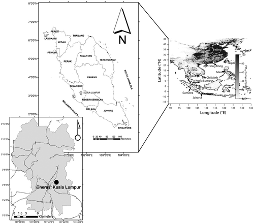
The sampling site is situated at Cheras (N03°06.376′, E101°43.072′, 43.4 m above sea level) in Kuala Lumpur, Malaysia. The station is located in a densely populated residential area with classification as an urban background station by the Department of Environment (DoE), Malaysia. The sampling station location is shown in Figure 1. Measurements started early February of 2004 and continued until December 2011. PM₁₀ concentration, precursor gases, as well as parameters related to the local meteorology—carbon monoxide (CO), ozone (O₃), oxides of nitrogen (NO_x), nitrogen oxide (NO), nitrogen dioxide (NO₂), sulfur dioxide (SO₂), methane (CH₄), nonmethane hydrocarbon (NMHC), wind speed (WS), wind direction (WDir), relative humidity (RH), and ambient temperature (T)—were measured. However, due to the unavailability of data for year 2011, CH₄ and NMHC were constructed for the period of 2004–2010 only.

Figure 1. Location of the sampling station at Cheras, Kuala Lumpur, and distribution of anthropogenic PM₁₀ emissions (30 min × 30 min resolution) in Southeast Asia in 2006 (data source: Zhang et al., 2009).

Measurement of PM₁₀ and atmospheric gases

PM₁₀ was measured continuously with a Met-One Beta Attenuation Monitor (BAM 1020; Washington, USA) aerosol mass monitor, which is certified by the U.S. Environmental Protection Agency. The BAM 1020 operation is based on beta-ray attenuation and provides real-time aerosol mass readings. The instrument has fairly high resolution of 0.1 μg m⁻³ at 16.7 L min⁻¹ flow rates with lower detection limits of <4.8 and <1.0 μg m⁻³ for 1 and 24 hr, respectively (www.metone.com). Details of the measurements of the precursor gases are presented in Table 1.

Table 1. Measurements of precursor gases

Variables	Instrument Model (Teledyne, USA)	Measurement Principle	Ranges	Precision	Lowest Detection Limit (LOD)
O3	Analyzer 400A	Chemiluminescence	0–100 ppb/0–10 ppm	0.5% (<10 s)	<0.6 ppb
NO, NO2, NOx	API 200A	Chemiluminescence	50–20,000 ppb	0.5%	0.4 ppb
SO2	API M100A	Florescence	50–20,000 ppb	0.5%	0.4 ppb
CO	API M300	Nondispersive infrared absorption	0–30 ppm/0–3000 ppm	0.5% (<10 s)	0.2 ppm
CH4/NMHC	API M4020	Flame ionization detector	—	1%	—

Quality control and quality assurance (QC/QA) for PM₁₀, trace gases, and meteorological measurement

Instruments used in in situ monitoring were managed by a private company named Alam Sekitar Sdn. Bhd. (ASMA). An autocalibration was scheduled for each instrument on a daily basis by which zero air calibration as well as standard cylinder gas was injected during the operation.

Multivariate and other statistical techniques

Advanced principal component analysis (PCA) is a robust driving tool for source apportionment and quantitative estimation of PM₁₀ sources. PCA combined with APCS is used extensively for prediction and estimation of source strength in ambient aerosols (Thurston and Spengler, 1985; Harrison et al., 1996). A stepwise and detailed procedure for the PCA-APCS calculation has been explained in previous studies (Khan et al., 2010, 2012). As local meteorology governs the strength of the sources of PM₁₀, we include the major meteorological factors in this apportionment, as in Juda-Rezler et al. (2011) and Viana et al. (2006). In order to achieve linearity of the data, wind vectors were resolved into their horizontal and vertical components.

The measurements contain missing values. Imputation methods suggest various ways to replace the missing values with plausible values. Missing data have been replaced with the mean value of each variable. Mean substitution technique is recommended be used when the missing data were less than 10% of the measurement (Trikriktsis, 2005). The suitability and adequacy of the data set for PCA was verified with the Kaiser-Meyer-Olkin (KMO) test. Taner et al. (2013) suggested that a sample data set will be adequate and recognizable if the KMO value is greater than 0.5. Our KMO value was 0.8, which is consistent with Taner et al. (2013). The data sets of trace gases and meteorological parameters were normalized and subjected to PCA varimax rotation. The number of factors was optimized based on the eigenvalue (>1). Additionally, PCA was used based on the number of factors and sensitivity of each variable to factor loading during the optimization process.

Results and Discussion

Time series of PM₁₀ and atmospheric trace gases

Concentrations of PM₁₀ and trace gases are summarized in Table 2. The concentrations have been divided into two categories: (i) weekdays and (ii) weekends. The overall mean concentration of the PM₁₀ for 8 yr of hourly data is 51.3 ± 28.5 μg m⁻³ and the annual average is 51.6 ± 25.8 μg m⁻³. The annual average concentration exceeds the annual PM₁₀ concentrations in the Recommended Malaysian Air Quality Guidelines (RMAQG) and in international standards, for example, the World Health Organization (WHO) air quality guidelines and the European Union (EU) air quality standards. The recommended air quality guideline set by the Malaysian government is 50 μg m⁻³ annually. The EU has set a lower value of 40 μg m⁻³ for yearly PM₁₀ mass (European Commission, 2013). The WHO, on the other hand, announced stricter recommendations as low as 20 μg m⁻³ for annual PM₁₀ to maintain better urban air quality (WHO, 2005).

Table 2. Summary statistics of measured data at Cheras station, Kuala Lumpur

Parameter	Valid N			Mean ± SD			Median			Min			Max
	Overall	WD	WE	Overall	WD	WE	Overall	WD	WE	Overall	WD	WE	Overall	WD	WE
PM10 (μg m^−3)	67229	47958	19271	51.3 ± 28.5	52.1 ± 29.7	49.2 ± 25.3	46.0	47.0	45.0	5.0	5.0	5.0	879.0	879.0	359.0
CO (ppbv)	63710	45294	18416	940.7 ± 674.8	950.9 ± 674.3	915.5 ± 675.2	760.0	780.0	740.0	10.0	10.0	10.0	7440.0	7440.0	6400.0
O3 (ppbv)	57178	40667	16511	20.5 ± 25.1	20.5 ± 25.3	20.5 ± 24.6	8.0	8.0	9.0	1.0	1.0	1.0	196.0	196.0	172.0
SO2 (ppbv)	60068	42873	17195	2.4 ± 2.0	2.5 ± 2.0	2.3 ± 1.9	2.0	2.0	2.0	1.0	1.0	1.0	66.0	52.0	66.0
NOx (ppbv)	64143	45587	18556	40.5 ± 31.4	40.8 ± 31.0	39.6 ± 32.3	32.0	33.0	31.0	1.0	1.0	1.0	353.0	353.0	294.0
NO (ppbv)	59038	42044	16994	21.0 ± 26.3	20.9 ± 25.8	21.4 ± 27.5	9.0	9.0	9.0	1.0	1.0	1.0	323.0	323.0	253.0
NO2 (ppbv)	64079	45549	18530	21.2 ± 11.9	21.6 ± 12.2	20.0 ± 11.4	19.0	19.0	18.0	1.0	1.0	1.0	112.0	93.0	112.0
CH4 (ppbv)	46899	33268	13631	2097.2 ± 305.9	2089.8 ± 295.4	2115.2 ± 329.6	2050.0	2040.0	2060.0	1500.0	1500.0	1500.0	7290.0	7290.0	6140.0
NMHC (ppbv)	46795	33202	13593	421.0 ± 311.2	425.6 ± 310.9	410.0 ± 311.8	350.0	350.0	330.0	10.0	10.0	10.0	3110.0	3110.0	2320.0
WS (km hr^−1)	68431	—	—	4.0 ± 2.9	—	—	3.3	—	—	0.8	—	—	102.0	—	—
T (°C)	62158	—	—	27.4 ± 3.5	—	—	26.1	—	—	20.9	—	—	39.0	—	—
RH (%)	67136	—	—	84.1 ± 15.6	—	—	88.0	—	—	29.0	—	—	100.0	—	—

Notes: WD = weekdays; WE = weekend; SD = standard deviation; WS = wind speed; “—” = no data

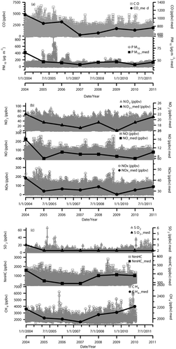
The overall average concentration of PM₁₀ on weekdays is higher (4%) than the concentration on weekends. This clearly shows the impact of vehicle numbers on PM₁₀ concentration. The concentration of ozone remained constant on weekdays and weekends. Ozone precursor concentration shows slight variation during the specified time periods. The degradation of trace gases in the atmosphere is dominated by their reaction with hydroxyl radical (OH). OH radicals are short-lived, and their formation and removal in the atmosphere are balanced. Reaction with ozone, nitric oxide, and hydrogen peroxide is the primary pathway of OH production and is consumed by a multitude of reaction with trace gases (Hofzumahaus et al., 2009). OH can remove almost all the pollutants, including CO and volatile organic compounds (VOCs). Reaction with CO and VOCs will produce hydroperoxy (HO₂) and organic peroxy (RO₂) radicals, respectively. With NO_x present in the air, RO₂ reacts with NO to produce HO₂. OH radical is re-formed by a reaction between HO₂ and NO with NO₂ as a by-product that degrades photochemically to produce ozone. Figure 2 depicts the time series of PM₁₀ concentration and the trace gases. Episodes of high concentration of CO are observed during the years 2004–2005. In contrast, episodes of high concentration of PM₁₀ are seen at the end of 2005. However, PM₁₀ high concentration patterns do not match the ozone precursor concentration patterns. Ozone precursors are known to affect aerosol concentration indirectly. NO, for example, is scavenged photochemically, a few minutes after emission (Kemp and Palmgren, 1996). CH₄ and NMHC, on the other hand, show no clear seasonal variations. These two trace gases are believed to be the O₃ precursor gases (Duan et al., 2008) where NMHC participates in the formation of secondary organic aerosols (Cocker et al., 2001). Thus, CH₄ and NMHC indirectly affect the variability of aerosol concentration (e.g., PM₁₀).

Figure 2. Time-series plots of PM₁₀, CO, NO, NO₂, NO_x, SO₂, CH₄, and NMHC using 1-hr and yearly median for 2004–2011.

Local meteorology

As summarized in Table 2, the average temperature was 27.4 °C, with a variation between 20.9 and 39.0 °C. The minimum and maximum relative humidity were 29% and 100%, with an average of 84%. Wind speed was on average of 4 km/hr. The synoptic wind field is shown in Figure 3. The wind over the Malaysian Peninsula generally blows from the northeasterly (NE) direction during November to March (Figure 3) and from the southwesterly (SW) direction June to September (Figure 3). The diurnal variations for T, RH, WS, and WDir are shown in Figure 4a. Temperature and relative humidity show an opposite diurnal cycle pattern. Temperature starts to increase from 8:00 a.m. local time (LT) and peaks at 2:00 p.m. LT. On the other hand, the RH shows downward trend from 8:00 a.m. LT to 2:00 p.m. LT, reaches 90% at 12:00 a.m. LT, when the ambient temperature at the lowest. The air was dry and warm in the afternoon.

Figure 3. Climatic wind stream and velocity at 10 m using ERA interim reanalysis data.

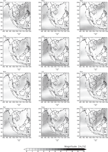
Figure 4. Diurnal plots of PM_10, meteorological factors and major air pollutants in 2004–2011 (overall average, weekday [WD], weekend [WE], and WE/WD ratio).

Diurnal patterns of PM₁₀ and trace gases

The diurnal variations of PM₁₀ concentrations, the trace gases, and meteorological parameters are shown in Figure 4a–j. Initially, the entire database for each of the parameters was re-sorted based on an overall data, weekdays (WD), and weekend (WE), which then were summarized as the 24-hr average. Their ranges per day were also extracted. Subgrouping of the database was considered to identify WE effect, if any. The diurnal concentration of PM₁₀ ranges from 45.7 to 59.5 μg m⁻³ with an average mass concentration of 51.3 μg m⁻³. PM₁₀ concentration during the WD ranged between 45.6 and 60.8 μg m⁻³, with the diurnal average of 52.1 μg m⁻³. With small difference, PM₁₀ concentration during the WE ranged from 41.5 to 60.7 μg m⁻³, with an average of 49.2 μg m⁻³ for the diurnal WE mass. The trend shows the highest in 2004 and then decreases gradually in the next 8 hr. PM₁₀ concentration shows significant variation during the 8-hr monitoring period, as previously shown in Figure 2. However, the trend of diurnal distribution for all subgroups (WD, WE, and overall data) of PM₁₀ concentration shows similar behavior. The concentration of PM₁₀ from 9:00 a.m. to 12:00 a.m. LT on the WD is somewhat higher (5–15%) as compared with the WE. Two distinct lowest hourly concentration were recorded at 07:00 a.m. LT and 2:00 p.m. LT; followed by a sharp peak at about 9:00 a.m. and 12:00 a.m. LT. The peak at 9:00 a.m. LT is caused by the traffic volume frequency during the morning rush hour, whereas the 12:00 a.m. peak is due to the temperature inversion.

Temperature inversion is a physical process that leads to the variability of PM₁₀ loading in the ambient air (Monks et al., 2009). The stagnant atmospheric conditions from 9:00 p.m. LT to 03:00 a.m. LT favors the accumulation of PM₁₀. At the same time, a temperature inversion and stable conditions prevail, which eventually stabilize the air mass and reduce the dispersion. This process normally occurs during stable atmospheric conditions (Galindo et al., 2013). However, the wind speed in general increase substantially from 10:00 a.m. to 5:00 p.m. LT (Figure 4a), which disperses PM₁₀. Similarly, a dilution effect could be observed in the deeper planetary boundary layer (PBL), where having a somewhat higher ambient and surface temperature, as well as a higher wind speed, will considerably lower the concentration of aerosols (Watson, 2002; Pitz et al., 2003; Chow et al., 2008; Barmpadimos et al., 2011).

O₃ shows a unimodal diurnal pattern (Figure 4e). Around 2:00 p.m. LT, O₃ concentration reaches its peak and soon thereafter starts to drop until 12:00 a.m. LT. The reactive oxygen (O) formed from reaction step 5 (R5) under an extended level of ultraviolet radiation leads to chemical conversion into O₃ in the presence of O₂ and bulk constituent (M) as in step 7 (R7). The reaction in steps 5 and 6 (R5 and R6) are also actively involved in the generation of surface-level O₃ (Seinfeld and Pandis, 2006; Lin et al., 2011). This is known as a key heterogeneous reaction, which takes place in the middle of the day. A similar change in O₃ with an afternoon maximum and a night time minimum were observed in another study in Malaysia (Toh et al., 2013). The diurnal plots of WD and WE coincide, suggesting that reaction step 5 (R5) (Figure 5) is primarily responsible for the generation of surface O_3. O₃ actively interferes in the formation of aerosol mass (R12). As seen in Figure 4b, the peak during the morning hours is the most significant and comes from the rush hour traffic. CO and SO₂ have similar bimodal distributions.

Figure 5. Pathways of heterogeneous reactions of atmospheric trace gases.

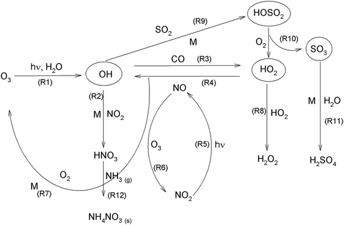
The mean NO concentration is 20.0 ppb_v, with the lowest concentration at 2.9 ppb_v and the highest concentration at 50.3 ppb_v. NO is released into the atmosphere from primary emission sources. NO₂, on the other hand, is generally formed in the atmosphere through photochemical conversion of NO. In this study, the mean concentration of NO₂ is 21.5 ppb_v, with lowest and highest concentrations being 12.3 and 32.9 ppb_v, respectively. NO₂ increases up to maximum of 96% during night due to the night time temperature inversion. Stable and stagnant conditions during night favor the formation of NH₄NO₃, when the relative humidity is high and the temperature is low (Stockwell et al., 2000). The stable forms of NO₃⁻ and NH₄⁺ (and in ambient aerosols; i.e., NH₄NO₃) form the gaseous-phase equilibrium of ammonia (NH₃) and nitric acid (HNO₃) via reaction step 12 (R12) (Figure 5) (Finlayson-Pitts and Pitts, 2000). The conversion of NO₂ produces most particulate-phase NO₃⁻ (Khoder, 2002), which contributes to the increased night time PM₁₀ level, as explained by reaction step 2 (R2) (Figure 5). The heterogeneous reaction steps (R2, R4, R5, and R6) in the above explanation are mainly responsible for this conversion (Figure 5). Therefore, the oxides of nitrogen are responsible for generating aerosol mass.

Irrespective of the season, the diurnal change in CH₄ concentration shows consistent decrease from 08:00 a.m. LT until 2:00 p.m. LT. NMHC concentration shows downward trend after reaching the peak at 9:00 a.m. The lower level of CH₄ and NMHC during middle of the day is due to several recognized photochemical reactions. However, there is no clear evidence of the role of CH₄ and NMHC in the formation of PM₁₀.

Trajectory analysis and impact of regional emission

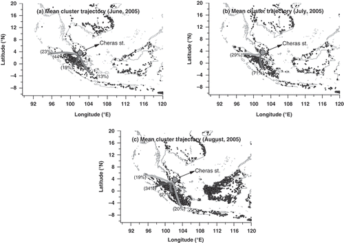
The concentration of PM₁₀ during the SW monsoon is typically high. We constructed a 72-hr cluster monthly mean backward trajectories at 500 m above sea level and 12:00 a.m. (UTC [coordinated universal time]) (Figure 6) using the Hybrid Single Particle Lagrangian Integrated Trajectory (HYSPLIT) model (Draxler and Rolph, 2013). Moderate Resolution Imaging Spectroradiometer (MODIS) fire data representing biomass burning hot spots in the specific area of interest were downloaded from the National Aeronautics and Space Administration (NASA) LANCE FIRMS¹ fire archive (http://firms.modaps.eosdis.nasa.-gov/download/) in the range of 8°S to 20°N and 90°W to 120°E. This has been appended to the graphs of the backward trajectories. By considering the percentage of mean cluster trajectories, the air mass is found to originate from regional sources. Most of the trajectories originated from Sumatra, Indonesia. Biomass hot spots are also found densely distributed in the Indonesian region (Figure 6), particularly during the southwesterly monsoon. The synoptic wind field shows that wind blows from the same region during the southwesterly monsoon (Figure 3).

Figure 6. Mean cluster of HYSPLIT back trajectory plots (500 m above sea level and 12:00 a.m. UTC) annotating MODIS fire hot spot counts.

Source characterizations

By means of PCA-APCS, three source fingerprints has been identified when the eigenvalue is set to 1, as shown in Figure 7a. The principal components of the three fingerprints (PC1, PC2, and PC3) accounted for 42%, 14%, and 8% of the total variance, respectively. In total, 64% of the variance can be explained in terms of the three PC factors identified. PC1 represents the major tracers CO, NO_x, NO, NO₂, and NMHC. Transportation is the main source of CO emission in Malaysia (Streets et al., 2003; Zhang et al., 2009). Incomplete combustion of fossil fuels is the primary source of CO. The process includes several reactions in the atmospheric gas phase, which indirectly affects the formation of aerosol particles, as shown in Figure 5. Similarly, NO_x is mainly emitted from combustion sources. Urban road traffic is believed to have contributed to the secondarily generated inorganic aerosol through the release of NO_x (Kumar et al., 2008). Mostly released from vehicles, NO is the second largest contributor to PM₁₀ concentration in Malaysia (Streets et al., 2003; Zhang et al., 2009). However, the forest and grassland fires also emit oxides of nitrogen (NO₂) (Carlo et al., 2015). Hence, PC1 can be identified as traffic emissions and contributes most significantly to PM₁₀.

Figure 7. (a) Loading of PCA factors of PM₁₀ for the period of 2004–2010. (b) The linear correlation plot of measured and predicted PM₁₀.

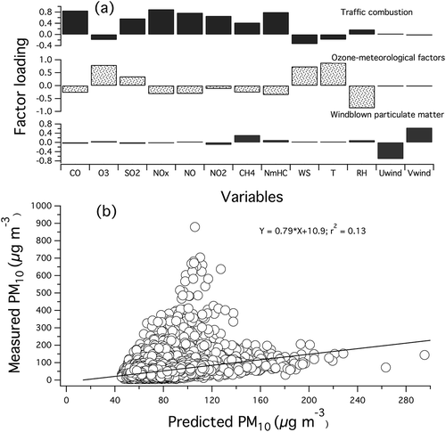
PC2 is associated with O₃, WS, T, and RH. Ozone is released into ambient air through photochemical reactions, mostly during the day. It is important to distinguish this principal component, as few of the potential meteorological parameters are grouped together. Wind speed, T, and RH are significant factors in a wider sense, as they govern the transport as well as the transformation of the gas into aerosol particles. Wind speed is inversely proportional to PM₁₀ mass, which suggests better ventilation or dispersion of aerosols (Zoumakis, 1998; Petrakakis et al., 2006). Van Poppel et al. (2012) found that the concentration of aerosol particles exponentially decreases with WS. Similarly, lower temperature and higher percentage of relative humidity affect the variability of PM₁₀ through the growth of aerosol particles (Hinds, 1999; Seinfeld and Pandis, 2006; Tsai et al., 2011). Thus, PC2 is defined as ozone and meteorological factor.

Wind vector resolved into horizontal and vertical components is the major contributor in PC3 (Figure 7a). Wind direction significantly affects the concentration of aerosol particles in Malaysian region, as the polluted air mass is mostly transported during the NE and SW monsoons (Figure 3). In agreement with this factor profile, the results of the mean cluster trajectories indicate that the air masses originate from the Sumatra, Indonesia (Figure 6). Allen et al. (2007) have concluded that the wind direction can be used to find pollutant source and strength. Therefore, the downwind effect from the particular region plays a significant role in changing the concentration of PM₁₀. Consequently, PC3 is described as the windblown particulate matter.

Multiple linear regression analysis (MLRA) was applied to estimate the mass of each PC source contributing to PM₁₀, expressed as mass over air volume (μg m⁻³). PM₁₀ was treated as the dependent variable, and APCS were used as independent variables. PCA scores were resampled to absolute scores using APCS analysis (Thurston and Spengler, 1985; Harrison et al., 1996). The MLRA shows that the coefficient of determination (R²) is 0.21 (P < 0.01). By comparing the total mass associated with the three factors and the constant, the PCA-APCS-MLRA overestimated the PM₁₀ by 2.0 μg m⁻³ or 4%. To evaluate the results of PCA-APCS-MLRA analysis, the predicted total mass of each source was regressed over the measured PM₁₀ mass. A linear correlation with slope value of 0.79, intercept of 10.9, and R² of 0.13 (Figure 7b) was produced. Hence, proof that the application of PCA-APCS-MLRA was effective in this study. The overall mass contributions of the identified PCs in percentage value are shown in Figure 8a. The average mass of the PC1 is 14.9 ± 13.1 μg m⁻³, with a range of 0.0005–150.4 μg m⁻³ or 28% of the average mass. Combustion from motor vehicles has been identified as the dominant among the PM₁₀ sources. PC2 and PC3 portion 10.9 ± 3.3 μg m⁻³ (20%) and 0.7 ± 0.2 μg m⁻³ (1%) of the average mass, respectively. The ranges of mass concentration for PC2 and PC3 are 5.1–43.8 and 0.2–2.1 μg m⁻³, respectively. However, the source apportionment analysis left 28.0 μg m⁻³ or 51% of the PM₁₀ concentration unexplained.

Figure 8. (a) Contribution of the PM₁₀ sources using PCA-APCS-MLRA. (b) The time series of the predicted contribution of PM₁₀ sources.

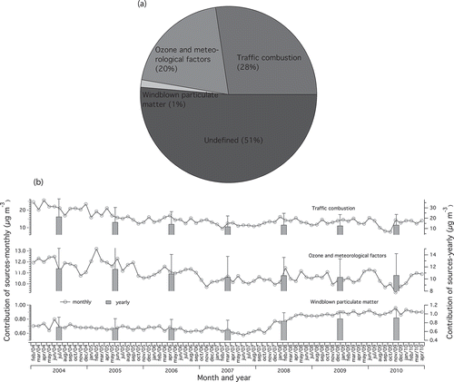
The trend of the yearly mean contribution of each source is shown in Figure 8b. PC1 source show variability in the monthly time series plot. A similar change is also observed for PC2 source. Windblown particulate matter sharply increased from January 2008 to November 2009. The above changes were prominent during both the southwesterly and northeasterly monsoons.

Conclusions

The effects of physicochemical factors on PM₁₀ concentration were analyzed, and the aerosol sources were characterized using 1-hr resolution data measured over 8 yr at Cheras station in Kuala Lumpur, Malaysia. The yearly average of PM₁₀ was 51.3 ± 25.8 μg m⁻³, which exceeds all major standards set by the RMAQG, WHO, and the EU. The back-trajectory analysis and biomass fire hot spots revealed that the highest frequency of haze pollution occurred in 2005, which contributed to the increase in PM₁₀ concentration. The PCA-APCS-MLRA analysis identified traffic combustion as the predominant source of PM₁₀, covering 28% of the total mass. The concentration of PM₁₀ is also dependent on the number of vehicles, with high levels observed during the morning rush hour. Meteorological factors, ozone, and precursors of ozone have significant effect on PM₁₀ concentration. High relative humidity and low temperature are linked to high PM₁₀ concentration. Additionally, wind speed can disperse the concentration of aerosols. High PM₁₀ concentration during the southwest monsoon is due to the particles being transported from areas of biomass burning in Sumatra.

Acknowledgment

The authors would like to thank the Malaysian Department of the Environment (DoE) for providing air quality data in the process of conducting research. We also would like to thank to the National Oceanic and Atmospheric Administration (NOAA) Air Resources Laboratory for the provision of the HYSPLIT transport and dispersion model and/or READY Web site (http://www.arl.noaa.gov/ready.html) used in this investigation. Special thanks to K. Alexander for proofreading the manuscript.

Funding

The authors would like to thank Universiti Kebangsaan Malaysia for Research University Grant (DIP-2014-005).

ORCID

Md. Firoz Khan

http://orcid.org/0000-0003-3567-9634

Additional information

Funding

The authors would like to thank Universiti Kebangsaan Malaysia for Research University Grant (DIP-2014-005).

Notes on contributors

Firoz Khan

Md. Firoz Khan is a university lecturer at the Centre for Tropical Climate Change System, Institute of Climate Change, Universiti Kebangsaan Malaysia, Bangi, Selangor, Malaysia.

Mohd Talib Latif

Mohd Talib Latif is a professor at the Centre for Tropical Climate Change System, Institute of Climate Change, and the School of Environmental and Natural Resource Sciences, Faculty of Science and Technology, Universiti Kebangsaan Malaysia, Bangi, Selangor, Malaysia.

Liew Juneng

Liew Juneng and Mohd Shahrul Mohd Nazdir are senior lecturers and Hossain Mohammed Syedul Hoque is a Ph.D. student at the School of Environmental and Natural Resource Sciences, Faculty of Science and Technology, Universiti Kebangsaan Malaysia, Bangi, Selangor, Malaysia.

Norhaniza Amil

Norhaniza Amil is a Ph.D. student at the School of Environmental and Natural Resource Sciences, Faculty of Science and Technology, Universiti Kebangsaan Malaysia, Bangi, Selangor, Malaysia, and the School of Industrial Technology (Environmental Division), Universiti Sains Malaysia, Penang, Malaysia.

Notes

Land, Atmosphere Near real-time Capability for EOS (Earth Obserserving System) Fire Information for Resource Management System.

References

- Allen, C.T., G.S. Young, and S.E. Haupt. 2007. Improving pollutant source characterization by better estimating wind direction with a genetic algorithm. Atmos. Environ. 41:2283–2289. doi:10.1016/j.atmosenv.2006.11.007
- Banan, N., M.T. Latif, L. Juneng, and F. Ahamad. 2013. Characteristics of surface ozone concentrations at stations with different backgrounds in the Malaysian Peninsula. Aerosols Air Qual. Res. 13:1090–1106. doi:10.4209/aaqr.2012.09.0259
- Barmpadimos, I., C. Hueglin, J. Keller, S. Henne, and A.S.H. Prévôt. 2011. Influence of meteorology on PM10 trends and variability in Switzerland from 1991 to 2008. Atmos. Chem. Phys. 11:1813–1835. doi:10.5194/acp-11-1813-2011
- Chow, J.C., P. Doraiswamy, J.G. Watson, L.W.A. Chen, S.S.H. Ho, and D.A. Sodeman. 2008. Advances in integrated and continuous measurements for particle mass and chemical composition. J. Air Waste Manage. Assoc. 58:141–163. doi:10.3155/1047-3289.58.2.141
- Chow, J.C., J.G. Watson, D.H. Lowenthal, R.T. Egami, P.A. Solomon, R.H. Thuillier, K. Magliano, and A. Ranzieri. 1998. Spatial and temporal variations of particulate precursor gases and photochemical reaction products during SJVAQS/AUSPEX ozone episodes. Atmos. Environ. 32:2835–2844. doi:10.1016/S1352-2310(97)00449-4
- Carlo, P.D., E. Aruffo, F. Biancofiore, M. Busilacchio, G. Pitari, C.D. Salisburgo, P. Tuccella, and Y. Kajii. 2015. Wildfires impact on surface nitrogen oxides and ozone in Central Italy. Atmos. Pollut. Res. 6:29–35. doi:10.5094/APR.2015.004
- Cocker, D.R., III, B.T. Mader, M. Kalberer, R.C. Flagan, and J.H. Seinfeld. 2001. The effect of water on gas–particle partitioning of secondary organic aerosol: II. m-Xylene and 1,3,5-trimethylbenzene photooxidation systems. Atmos. Environ. 35:6073–6085. doi:10.1016/S1352-2310(01)00405-8
- Dominick, D., H. Juahir, M.T. Latif, S.M. Zain, and A.Z. Aris. 2012. Spatial assessment of air quality patterns in Malaysia using multivariate analysis. Atmos. Environ. 60:172–181. doi:10.1016/j.atmosenv.2012.06.021
- Draxler, R.R., and G.D. Rolph. 2013. HYSPLIT (HYbrid Single-Particle Lagrangian Integrated Trajectory) Model access via NOAA ARL READY Web site. NOAA Air Resources Laboratory, Silver Spring, MD. http://ready.arl.noaa.gov/HYSPLIT.php (accessed September 15, 2013).
- Duan, J., J. Tan, L. Yang, S. Wu, and J. Hao. 2008. Concentration, sources and ozone formation potential of volatile organic compounds (VOCs) during ozone episode in Beijing. Atmos. Res. 88:25–35. doi:10.1016/j.atmosres.2007.09.004
- Finlayson-Pitts, B.J., and J.N. Pitts Jr. 2000. Chemistry of the Upper and Lower Atmosphere: Theory, Experiments, and Applications. New York: John Wiley & Sons.
- Friend, A., G.A. Ayoko, D. Jager, M. Wust, R. Jayaratne, M. Jamriska, and L. Morawska. 2013. Sources of ultrafine particles and chemical species along a traffic corridor: Comparison of the results from two receptor models. Environ. Chem. 10:54–63. doi:10.1071/EN12149
- Galindo, N., J. Gil-Moltó, M. Varea, C. Chofre, and E. Yubero. 2013. Seasonal and interannual trends in PM levels and associated inorganic ions in southeastern Spain. Microchem. J. 110:81–88. doi:10.1016/j.microc.2013.02.009
- Harrison, R.M., D. Smith, and L. Luhana. 1996. Source apportionment of atmospheric polycyclic aromatic hydrocarbons collected from an urban location in Birmingham, UK. Environ. Sci. Technol. 30:825–832. doi:10.1021/es950252d
- Haywood, J., and O. Boucher. 2000. Estimates of the direct and indirect radiative forcing due to tropospheric aerosols: A review. Rev. Geophys. 38:513–543. doi:10.1029/1999RG000078
- Hinds, W.C. 1999. Aerosol Technology, Properties, Behavior, and Measurement of Airborne Particles, 2nd ed. New York: John Wiley & Sons.
- Hofzumahaus, A., F. Rohrer, L. Keding, B. Bohn, T. Brauers, C.-C. Chang, H. Fuchs, F. Holland, K. Kita, Y. Kondo, Y., et al. 2009. Amplified trace gas removal in the troposphere. Science 324:1702–1704. doi:10.1126/science.1164566
- Juda-Rezler, K., M. Reizer, and J.P. Oudinet. 2011. Determination and analysis of PM10 source apportionment during episodes of air pollution in Central Eastern European urban areas: The case of wintertime 2006. Atmos. Environ. 45:6557–6566. doi:10.1016/j.atmosenv.2011.08.020
- Juneng, L., M.T. Latif, and F. Tangang. 2011. Factors influencing the variations of PM10 aerosol dust in Klang Valley, Malaysia during the summer. Atmos. Environ. 45:4370–4378. doi:10.1016/j.atmosenv.2011.05.045
- Kemp, K., and F. Palmgren. 1996. The Danish urban air quality monitoring program: Objectives and results. Sci. Total Environ. 189–190:27–34. doi:10.1016/0048-9697(96)05187-X
- Khan, M.F., K. Hirano, and S. Masunaga. 2010. Quantifying the sources of hazardous elements of suspended particulate matter aerosol collected in Yokohama, Japan. Atmos. Environ. 44:2646–2657. doi:10.1016/j.atmosenv.2010.03.040
- Khan, M.F., K. Hirano, and S. Masunaga. 2012. Assessment of the sources of suspended particulate matter aerosol using US EPA PMF 3.0. Environ. Monit. Assess. 184:1063–1083. doi:10.1007/s10661-011-2021-y
- Khoder, M.I. 2002. Atmospheric conversion of sulfur dioxide to particulate sulfate and nitrogen dioxide to particulate nitrate and gaseous nitric acid in an urban area. Chemosphere 49:675–684. doi:10.1016/S0045-6535(02)00391-0
- Kumar, P., P. Fennell, and R. Britter. 2008. Measurements of particles in the 5–1000 nm range close to road level in an urban street canyon. Sci. Total Environ. 390:437–447. doi:10.1016/j.scitotenv.2007.10.013
- Latif, M., S. Azmi, A. Noor, A. Ismail, Z. Johny, S. Idrus, A. Mohamed, and M. Mokhtar. 2011 The impact of urban growth on regional air quality surrounding the Langat River Basin, Malaysia. Environmentalist 31:315–324. doi:10.1007/s10669-011-9340-y
- Lee, Y.J., Y.W. Lim, J.Y. Yang, C.S. Kim, Y.C. Shin, and D.C. Shin. 2011. Evaluating the PM damage cost due to urban air pollution and vehicle emissions in Seoul, Korea. J. Environ. Manage. 92:603–609. doi:10.1016/j.jenvman.2010.09.028
- Lin, W., X. Xu, B. Ge, and X. Liu. 2011. Gaseous pollutants in Beijing urban area during the heating period 2007–2008: Variability, sources, meteorological, and chemical impacts. Atmos. Chem. Phys. 11:8157–8170. doi:10.5194/acp-11-8157-2011
- Monks, P.S., C. Granier, S. Fuzzi, A. Stohl, M.L. Williams, H. Akimoto, M. Amann, A. Baklanov, U. Baltensperger, I. Bey, et al. 2009. Atmospheric composition change—Global and regional air quality. Atmos. Environ. 43:5268–5350. doi:10.1016/j.atmosenv.2009.08.021
- Petrakakis, M.I., A.G. Kelessis, N.M. Zoumakis, and F.K. Vosniakos. 2006. PM10 concentrations in the urban area of Thessaloniki, Greece. Fresenius Environ. Bull. 11:499–504.
- Pitz, M., J. Cyrys, E. Karg, A. Wiedensohler, H.E. Wichmann, and J. Heinrich. 2003. Variability of apparent particle density of an urban aerosol. Environ. Sci. Technol. 37:4336–4342. doi:10.1021/es034322p
- Pope, C., III, and D.W. Dockery. 2006. Health effects of fine particulate air pollution: Lines that connect. J. Air Waste Manage. Assoc. 56:709–742. doi:10.1080/10473289.2006.10464485
- Pope, C.A., M. Ezzati, and D.W. Dockery. 2009. Fine-particulate air pollution and life expectancy in the United States. N. Engl. J. Med. 360:376–386. doi:10.1056/NEJMsa0805646
- Ramanathan, V., P.J. Crutzen, J.T. Kiehl, and D. Rosenfeld. 2001. Aerosols, climate, and the hydrological cycle. Science 294:2119–2124. doi:10.1126/science.1064034
- Seinfeld, J., and S.N. Pandis. 2006. Atmospheric Chemistry and Physics: From Air Pollution to Climate Change. New York: John Wiley & Sons.
- Stockwell, W.R., J.G. Watson, N.F. Robinson, W. Steiner, and W.W. Sylte. 2000. The ammonium nitrate particle equivalent of NOx emissions for wintertime conditions in Central California’s San Joaquin Valley. Atmos. Environ. 34:4711–4717. doi:10.1016/S1352-2310(00)00148-5
- Streets, D.G., T.C. Bond, G.R. Carmichael, S.D. Fernandes, Q. Fu, D. He, Z. Klimont, S.M. Nelson, N.Y. Tsai, M.Q. Wang, et al. 2003. An inventory of gaseous and primary aerosol emissions in Asia in the year 2000. J. Geophys. Res. Atmos. 108:8809. doi:10.1029/2002JD003093
- Taner, S., B. Pekey, and H. Pekey. 2013. Fine particulate matter in the indoor air of barbeque restaurants: Elemental compositions, sources and health risks. Sci. Total Environ. 454–455:79–87. doi:10.1016/j.scitotenv.2013.03.018
- Thurston, G.D., and J.D. Spengler. 1985. A quantitative assessment of source contributions to inhalable particulate matter pollution in metropolitan Boston. Atmos. Environ. 19:9–25. doi:10.1016/0004-6981(85)90132-5
- Toh, Y.Y., S.F. Lim, and R. von Glasow. 2013. The influence of meteorological factors and biomass burning on surface ozone concentrations at Tanah Rata, Malaysia. Atmos. Environ. 70:435–446. doi:10.1016/j.atmosenv.2013.01.018
- Triktsis, N. 2005. A review of techniques for training, missing data in OM survey research. J. Oper. Manage. 24:53–62.
- Tsai, J.H., L.T.C. Chang, Y.S. Huang, and H.L. Chiang. 2011. Particulate composition characteristics under different ambient air quality conditions. J. Air Waste Manage. Assoc. 61:796–805. doi:10.3155/1047-3289.61.7.796
- Van Poppel, M., L. Int Panis, E. Govarts, J. Van Houtte, and W. Maenhaut. 2012. A comparative study of traffic related air pollution next to a motorway and a motorway flyover. Atmos. Environ. 60:132–141. doi:10.1016/j.atmosenv.2012.06.042
- Viana, M., X. Querol, A. Alastuey, J.I. Gil, and M. Menéndez. 2006. Identification of PM sources by principal component analysis (PCA) coupled with wind direction data. Chemosphere 65:2411–2418. doi:10.1016/j.chemosphere.2006.04.060
- Wallace, J., and P. Kanaroglou. 2009. The effect of temperature inversions on ground-level nitrogen dioxide (NO2) and fine particulate matter (PM2.5) using temperature profiles from the Atmospheric Infrared Sounder (AIRS). Sci. Total Environ. 407:5085–5095. doi:10.1016/j.scitotenv.2009.05.050
- Wan Mahiyuddin, W.R., M. Sahani, R. Aripin, M.T. Latif, T.-Q. Thach, and C.M. Wong. 2013. Short-term effects of daily air pollution on mortality. Atmos. Environ. 65:69–79. doi:10.1016/j.atmosenv.2012.10.019
- Watson, J.G. 2002. Visibility: Science and regulation. J. Air Waste Manage. Assoc. 52:628–713. doi:10.1080/10473289.2002.10470813
- World Health Organization. 2005. Health Risk of Particulate Matter from Long Range Transboundary Air Pollution. Geneva: World Health Organization.
- Zhang, Q., D.G. Streets, G.R. Carmichael, K.B. He, H. Huo, A. Kannari, Z. Klimont, I.S. Park, S. Reddy, J.S. Fu, et al. 2009. Asian emissions in 2006 for the NASA INTEX-B mission. Atmos. Chem. Phys. 9:5131–5153. doi:10.5194/acp-9-5131-2009
- Zoumakis, N.M. 1998. Characteristics of maximum concentrations from multiple point sources. J. Appl. Meteorol. 37:730–739. doi:10.1175/1520-0450(1998)037