Monitoring study of the near-road PM_2.5 concentrations in Maryland

Abstract

The Maryland State Highway Administration (SHA) monitoring program monitored the impact of vehicular emissions on the concentrations of the fine particles smaller than 2.5 microns (PM2.5). PM2.5 concentrations were monitored in close proximity to a highway in order to determine whether traffic conditions on the roadway impact concentrations at this location. The monitoring program attempted to connect monitored concentrations with the roadway traffic exhaust or with the other sources of PM2.5. PM2.5 concentrations were collected near the Capital Beltway (I-495/I-95) in Largo, Maryland. The monitoring program was launched on May 13, 2009 and continued through the end of 2012. Two co-located monitors, one for continuous PM2.5 measurements and the other for speciation measurements, were used in this program. Meteorological and traffic information was also continuously collected at or near the monitoring site. Additionally, data from the two other monitoring locations, one at the Howard University-Beltsville, MD and one at McMillan Reservoir, DC, was used for comparison with the data collected at the SHA monitoring location. The samples collected by the speciation monitor were analyzed at the RTI and DRI Laboratories to determine the composition and the sources of the collected PM2.5 samples. Based on the apportionment analysis, the contribution of roadway sources is about 12 to 17 percent of PM2.5 at the near-road site.

Implications: PM_2.5 monitoring at 150 m (approximately 500 feet) from a major highway in Maryland near Washington, DC, demonstrated that roadway traffic contributes to the total PM_2.5 concentration near the roadway, but the contribution at such distance is small, in the order of 12–17% of the total.

Introduction

Higher emissions from traffic cause higher public exposure to vehicle-related pollution. Emissions from motor vehicles and their impacts on the public exposed to them have been subject of research for several decades. However, as our knowledge of these emissions and their effects and controls accumulates and develops, different pollutants and different areas of concern come into focus. Several studies of near-road pollution were conducted in the recent years as the problem of adverse health effects of lengthy exposure to traffic emissions (especially from diesel-fueled vehicles) came into U.S. Environmental Protection Agency (EPA) and public attention. The strengthening of the U.S. air quality standards connected with traffic emissions (PM_2.5 [particulate matter with an aerodynamic diameter <2.5 μm] and NO₂ [nitrogen dioxide]) in the recent years is another indication of the heightened awareness of this pollution (EPA, 2012).

Almost one-third of the population in the United States either lives or spends significant portion of the day in the close vicinity of busy or congested roadways, one-fifth within one-third of a mile, and 10% within 300 feet (Rowangould, 2013). Health Effects Institute (HEI) review of traffic-related air pollution (2010) presented a comprehensive review of vehicle emission studies and assessments of vehicular pollution health impacts (HEI Panel, 2010). This review focused on the monitoring and modeling studies of motor-vehicle emissions in the urban environment and in close proximity to busy roadways in the United States and worldwide and the health impact.

Several major roadside EPA and Federal Highway Administration (FHWA) studies were conducted to measure concentrations and estimate public exposure to the vehicular emissions: in Brooklyn, New York (2004), in Raleigh, North Carolina (2008), in Las Vegas, Nevada (2010), and in Detroit, Michigan (2011). Roadside emissions and exposure to them were studied in many other monitoring and wind-tunnel assessments (Yoon, 2003; Baldauf et al., 2009, 2012; Black et al., 2009; Kimbrough et al., 2011; Ginzburg et al., 2012; Schattanek et al., 2012). These studies tried to determine which pollutants are common and most prevalent, which produced the most damaging health impacts, what are the effects of traffic emissions at different distances from roadway (Baldauf et al., 2008) and answer many other related questions. Pollutants that were studied included carbon monoxide, mobile source air toxics, black carbon and particulate matter, nitrogen oxides, and secondary formations. A few studies looked at the concentrations at various distances from the edge of the roadway (1998 Netherlands monitoring, 2002 Los Angeles study, 2008 Raleigh study, and 2010 Nevada study), but most field observations were limited either in time and/or in scope (HEI Panel, 2010). Other research was aimed at connecting collected data with the vehicular exhaust emissions to attribute monitored concentrations to the supposed source.

In the study of ultrafine particles near the major truck route (I-710) in Los Angeles, monitored particulate concentrations dropped sharply with distance from the roadway (Zhu et al., 2002). At a distance little more than 100 m (300 feet) away from the roadway, monitored concentrations were close to background concentrations. The 2012 study near the same roadway also looked at pollutant gradients downwind of a freeway carrying a high volume of diesel traffic (Zhou and Levy, 2007). This recent study confirmed the results of the previous study. The results obtained from this monitoring study suggest that motor-vehicle emissions from the I-710 increase the atmospheric concentration of most combustion-related pollutants above background levels, especially within the first 80 m (262.5 feet) from the edge of the freeway. Roadside concentrations of nitrogen oxides (NO_x), carbon monoxide (CO), and volatile organic compounds (VOCs) may be a factor of 2–4 higher than the community average ambient concentrations (Fujita et al., 2011). Heavy-duty diesel vehicles can increase these ratios to as much as a factor of 10 for NO_x and black carbon (Westerdahl, et al., 2005).

The Raleigh study monitored criteria pollutants including PM_2.5 and included black carbon among other pollutants (Baldauf et al., 2008). Among other results, this study demonstrated that peak-hour levels and daily concentration variation decreased with distance from the roadway. The monitoring project in Nevada studied mobile source air toxics (MSAT) criteria pollutants, including PM_2.5 and black carbon at 20–300 m (66–984 feet) from the roadway (Black, 2009). This study demonstrated that near-road concentration patterns are influenced by daytime turbulence. Similar results were obtained in the study of roadside concentrations of particulate matter in Chennai, India (Muruganandam and Nagendra, 2011). An analysis that processed data from 41 roadside monitoring studies from 1978 through 2008 normalized measured concentrations of several traffic-generated pollutants to either edge of the road concentration or the background (as reported in the studies) concentration (Karner et al., 2010). The decrease to background level was found from as close as 80–100 m (262.5–328 feet) to 160 m (525 feet). Another analysis of the data extracted from the published studies (Polidori and Fine, 2012) also found that road traffic emissions of particulate matter influence concentrations as far as 100–400 m (328–1312 feet) from the edge of the roadway (Zhou and Levy, 2007).

Current EPA research concentrates on examination of multipollutant environment and interference between different mobile source pollutants in the vicinity of busy roadways. The other area of current interest is pollution patterns in the complex terrain near roadways: near depressed roads, near obstacles, etc. The monitoring study presented in this study focused on one pollutant, PM_2.5, examined its impact at a single point location away from a high-volume interstate highway for a prolonged time period, and tried to apportion collected mass to the traffic emissions from this roadway.

Concentrations of particles smaller than 2.5 microns in diameter (PM_2.5) were collected at a monitoring site located in close proximity to a heavily traveled roadway for over 3½ yr to determine whether these concentrations can be correlated with local traffic and/or meteorological conditions. The Maryland State Highway Administration (SHA) monitoring program studied the impact of vehicular exhaust from highway traffic on the concentrations of the fine particulates to determine whether or not monitored concentrations came from roadway traffic or from the other sources of PM_2.5 such as residential or commercial heating and air conditioning, or other background sources. The monitoring program started on May 13, 2009, and continued for 3½ yr through the end of 2012, which allowed collection of sufficient number of valid measurements. The collected data were analyzed to determine whether and to what degree the PM_2.5 concentrations were affected by the traffic emissions.

Monitoring Program Setup

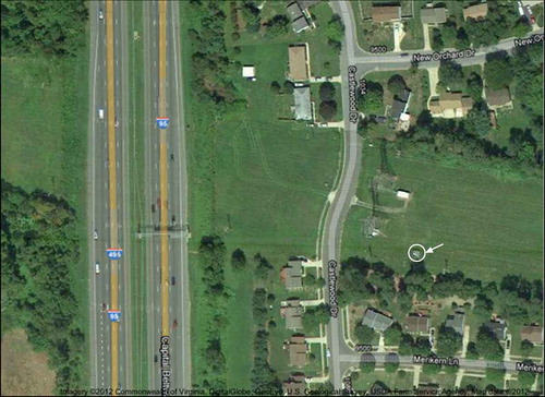
PM_2.5 concentrations were collected at a location 149 m (489 feet) from the edge of the Capital Beltway (I-495/I-95) near the MD 214 interchange in Largo, Maryland. The monitoring site was selected near a major highway (I-95) with high average daily traffic (ADT) volumes. The selected site complies with the EPA neighborhood siting criteria (EPA, 1998) in terms of distances from vehicular roadways and nearby obstacles. The site was located east of the Beltway to take advantage of the prevailing westerly winds (Figure 1).

Figure 1. Monitoring site location.

The monitoring study followed the recommended EPA procedures (EPA, 1999, 2006, 2011; Watson et al., 2011). Two monitors, one for continuous PM_2.5 measurements and the other for speciation measurements, both manufactured by Met One Instruments Inc., were used in this study. The continuous monitor, Beta Attenuation Mass Monitor (E-BAM) (Met One Instruments, Inc., 2014a), collected hourly samples; the speciation monitor, Super SASS (Met One Instruments, Inc., 2014b), operated on a 1-in-6-day schedule, with the collected samples sent to the Research Triangle Park (RTI) International laboratory and the Desert Research Institute (DRI) for chemical speciation and semivolatile organic analysis. Using the speciation data, DRI performed receptor modeling to determine, based on chemical composition, whether sources of the collected particulate matter can be identified. The monitors were located within a 12-foot by 12-foot fenced area secured with a lock. Each monitor was mounted on a secure tripod. Hardwired AC (alternating current) electric power was provided.

The following additional data were collected for use in this study:

1. Traffic volumes and speeds on the Capital Beltway were collected at approximately 0.50 km (0.31 mile) to the north of the monitoring site. The data collected at this location are representative of the traffic near the monitoring site because there are no exits to or from the Capital Beltway between the sensor location and the monitoring location.

2. Meteorological data (wind data, ambient temperature, and relative humidity) were collected at the PM_2.5 monitoring location on a continuous basis.

3. PM_2.5 concentrations were collected by the Maryland Department of the Environment (MDE) site at the Howard University (HU)-Beltsville monitor. This monitoring station is located approximately 3 km (1.6 miles) from I-95 (a major highway with an ADT count of 100,000 in 2008) and 500 m (0.3 mile) from US Route 1 (a local route that carries an ADT of 21,000). In addition, the HU-Beltsville monitor is separated from Route 1 by a forested area. There are two PM_2.5 monitors at this location: one for continuous PM_2.5 monitoring and one for speciation purposes.

4. PM_2.5 concentrations were collected near the McMillan Reservoir as part of the District of Columbia Department of Environment (DDOE) monitoring program. This monitor, which is intended for measuring the effects of vehicular emissions, is located 10.8 km (6.7 miles) from I-95, less than 300 m (0.2 mile) from Rhode Island Avenue, and approximately 800 m (0.5 mile) from Georgia Avenue in Washington, DC. Continuous and speciation PM_2.5 monitoring is conducted at this location.

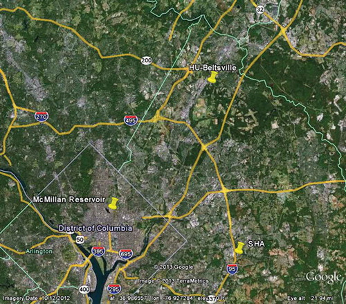
The relative locations of all three monitoring sites are presented on Figure 2. All three monitoring locations including the study location are at about the same elevation above the sea level, which is around 170 feet.

Figure 2. Monitoring site location relative to the comparison monitoring sites.

Data Collected

The program collected 29,647 hr (1234 days) of continuous PM_2.5 concentrations and 204 daily samples of data for speciation analysis. The data recovery rate for the continuous monitoring was 93%. PM_2.5 hourly concentrations collected by the E-BAM monitor were processed to determine daily (24-hr) average concentrations. The highest hourly monitored concentration for the entire period was 255 μg/m³. Table 1 presents the highest collected daily concentrations and the number of concentrations exceeding 35 µg/m³ in each calendar year. On 15 days during the monitored period, the measured concentration exceeded the level of 35 μg/m³, the level of the 24-hr National Ambient Air Quality Standard (NAAQS) for PM_2.5. However, this standard is set in the statistical form with design value comparable to the 3-yr average of the 98th percentile of the yearly 24-hr daily PM_2.5 concentrations. In the course of the monitoring program, the 98th percentile daily concentrations in each year except 2010 did not exceed 35 μg/m³. The 98th percentile average for the three calendar years in the monitoring period was 32.3 μg/m³, which is below the 24-hr NAAQS. The estimated annual PM_2.5 concentration for the three full years was 13.0 μg/m³, below the current PM_2.5 annual NAAQS of 15 μg/m³, but above the recently adapted stricter annual PM_2.5 standard of 12 μg/m³, which is planned to come in effect in 2015.

Table 1. Concentrations (μg/m³) by year

Parameter	2009*	2010	2011	2012
Maximum 24-hr concentration	39.9	40.3	41.4	41.0
98% concentration	27.9	36.6	33.0	31.7
Number of days >35 μg/m^3	2	7	4	2
Number of daily observations	229	337	364	304

Notes: *Monitoring program started on May 13, 2009.

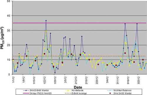
The tendency of the 24-hr total concentrations from the Super SASS monitor corresponded well with the tendency of the continuous monitoring concentrations collected with the E-BAM monitor, as illustrated on Figure 3 for the first quarter of 2012.

Figure 3. Daily PM_2.5 concentrations in the first quarter of 2012 (E-BAM and Super SASS at SHA site and continuous monitors at HU-Beltsville and McMillan sites).

The samples collected by Super SASS were sent to the RTI laboratory for chemical speciation and gravimetric analysis (Homolya and Rice, 1999). In addition, the quartz filter samples were combined by month, extracted, and analyzed for semivolatile organic compounds by the Organic Analysis Laboratory at the DRI. Using the resulting speciation data, the DRI performed source apportionment analyses using the Chemical Mass Balance (CMB-8) program to determine, based on chemical composition, whether sources of the collected particulate matter can be identified.

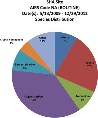
The speciation analyses for each month were summarized, and the summary for the period (Figure 4) indicated that the major elements of the collected PM_2.5 material were organic carbon (36%), sulfates (23%), nitrates (9%), elemental carbon (8%), and ammonium (9%).

Figure 4. Speciation results—major monitored elements.

The meteorological parameters were observed on an hourly basis, including wind speed and direction, ambient temperature, and relative humidity. A total of 39,376 hr were observed from May 13, 2009, through December 31, 2012, for the ambient temperature and humidity. The wind observations counted 30,444 hr for the same period.

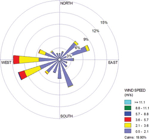
Wind speed and direction are presented on Figure 5. The strongest wind was 13.0 m/sec (29.1 miles per hour). One of reasons for the monitoring site selection was its location east of the Capital Beltway, downwind of the highway during prevailing westerly winds; however, since this region is in the path of low-pressure systems, wind directions change frequently. Prevailing winds from the southwest (that blow towards the monitoring site from I-95) were generally stronger than the winds in the direction away from the monitoring site (from east-northeast).

Figure 5. Speed and direction observed at the SHA monitoring site (2009–2012).

During the 29,647 monitoring hours, there were 1738 hr with precipitation. Half of the time the precipitation was not significant (with intensity lower than 0.04 inch per hour). No significant deterioration in the monitored PM_2.5 concentrations during the hours of precipitation was detected mostly because of low intensity of precipitation in bulk of the precipitation hours.

Volumes, speeds, and vehicle classification data were collected for the north- and southbound directions of the I-95 road section adjacent to the monitoring site. These traffic data are composed of information collected by NAVTEQ (Navigation Technology) traffic collection, (NAVTEQ, 2014) from May 13 through December 5, 2009, and by an ATR (Automatic Traffic Recorder; Maryland State Highway Administration, 2014) from December 6, 2009, through the end of the monitoring period. The NAVTEQ data contained only four vehicle classes and from these classes, the 13 classes that the ATR collects were projected using the historic data at this location. A set of correction factors were developed to convert the four classes of NAVTEQ traffic volume data into 13 classes of loop detector traffic volume data for each vehicle class for each day of the week on an hour-by-hour basis. In the last 2 months of 2012, the sensors for axle-based classification failed and were not repaired due to impending road resurfacing. The speeds and volumes by three length-based classes as opposed to 13 FHWA classes were collected for November–December 2012. Classification data were restored based on the length-based classes and historic data collected during the program.

The relevant results of the traffic data collected on I-95 are as follows:

1. Average annual daily traffic (AADT) volumes were approximately 205,291 vehicles.

2. Average vehicular speeds were 59–63 mph.

3. The maximum daily volume was 248,836 vehicles.

4. The peak hourly traffic volume was 16,454 vehicles.

5. Night traffic was lighter than the daytime traffic.

6. Heavy-duty vehicles constituted up to 6% of the daily traffic.

The nighttime total volumes are lower, but the heavy-duty trucks (HDTs) volume and percentage of HDTs in the total traffic volume are higher. Heavy-duty vehicles constituted around 13% of the nighttime traffic, with a maximum of from 22% to 33%.

Data Analysis

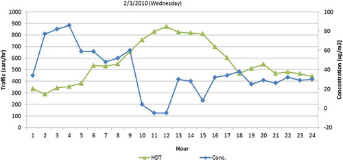
The collected data were analyzed to determine whether and to what degree the PM_2.5 concentrations were affected by the traffic emissions. The hourly data for the days exceeding 35 μg/m³ was plotted (see Figures 6 and 7) against the hourly traffic (total volume and HDTs) to see if there is a connection. The peak hourly concentrations that brought the 24-hr average above the reference level do not correspond to high traffic (or HDT) volumes as shown at Figures 6 and 7. Wind directions during peak hours were away from the monitoring site, otherwise the monitors would have register higher concentration during these hours. However, as shown below, wind directions do not have a high correspondence with the monitored concentrations at the SHA site.

Figure 6. Hourly PM_2.5 concentrations and traffic volumes.

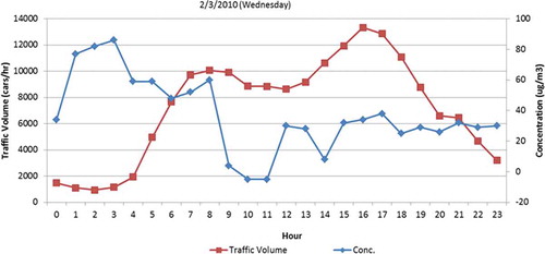
Figure 7. Hourly PM_2.5 concentrations and HDT traffic volumes.

Comparison of monitored PM_2.5 concentrations with Maryland Department of the Environment and District of Columbia Department of Environment sites

Hourly PM_2.5 concentrations at MDE’s Howard University–Beltsville and DDOE’s McMillan Reservoir monitors measured concurrently with the monitoring period of this study were compared with the data collected at the SHA monitor. Average and maximum 24-hr PM_2.5 concentrations at each of these monitors are provided in Table 2. The average hourly and daily concentrations at the SHA site were higher than at either the Howard University–Beltsville or McMillan Reservoir monitors. The standard deviation of concentrations monitored at the SHA station was also greater than at the other two locations.

Table 2. 24-Hour PM_2.5 concentrations (μg/m³) measured at continuous monitors

Parameter	SHA Monitor	Howard University–Beltsville	McMillan Reservoir
Average	13.0	11.6	10.3
Standard deviation	7.5	5.5	5.9
Maximum 24-hr concentration	41.4	39.6	41.5
Minimum 24-hr concentration	0.0	0.7	−0.3
Number of hourly observations	29,647	28,445	27,748

PM_2.5 concentrations and meteorological data

The 2009–2012 monitoring period data were roughly divided into two seasons: summer (May–September) and winter (October–December). Average hourly concentrations were plotted against average hourly ambient temperatures for these two seasons (Figures 8 and 9).

Figure 8. Diurnal variation of the ambient air temperature and monitored PM_2.5 concentrations during the summer season.

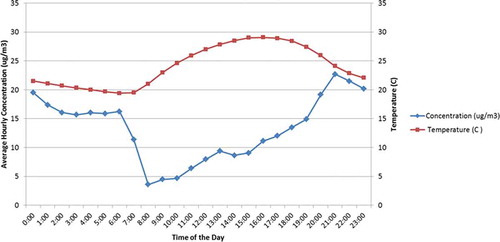
Figure 9. Diurnal variation of the ambient air temperature and monitored PM_2.5 concentrations during the winter season.

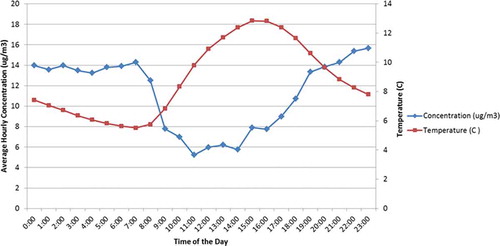
As shown, there appears to be an inverse relationship between concentrations and temperatures. The monitored data show that PM_2.5 concentrations are lower during the daytime (i.e., when traffic volumes are higher) than during the nighttime (when ambient air temperatures and traffic volumes are lower). Black carbon concentrations were also lower during the day in another study in Raleigh, North Carolina (Baldauf et al., 2008). Concentration variation is also greater in the summer season when temperature variations are also greater.

Atmospheric buoyancy could be a factor affecting pollutant concentrations during daytime and nighttime periods. Daytime turbulence increases mixing and dispersion and decreases PM_2.5 concentrations. In the nighttime, more stable atmospheric conditions diminish dispersion and cause higher PM_2.5 concentrations. Wind speeds associated with turbulence and atmospheric stability could be another factor associated with pollutant concentrations under daytime and nighttime periods.

No significant correlation of measured concentrations with wind direction was found, perhaps due to the distance from the roadway traffic to the monitor location. Correlation with wind speed from all directions was tested along with the correlation with only westerly winds (i.e., from the roadway to the monitor). Some correlation with the wind speed was found when only winds blowing directly from the roadway towards the monitor (i.e., 247.5°–292.5°) were considered. Concentrations were found to decrease with the increase in the wind speeds. This was a result of the increase in the atmospheric turbulence. Similar results were obtained in earlier studies.

PM_2.5 concentrations and traffic data

Monitored PM_2.5 concentrations were compared with traffic volumes collected along a section of the Capital Beltway near the monitoring site. The local roads around the site have very low AADT, which was not taken into account. Figures 10 and 11 present average hourly concentrations and average hourly traffic volumes. The traffic volumes presented are either total volumes (i.e., in both directions) or HDT volumes (in both directions).

Figure 10. Average hourly traffic volumes and monitored PM_2.5 concentrations.

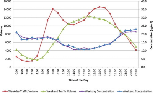
Figure 11. Average hourly heavy-duty vehicle volumes and monitored PM_2.5 concentrations.

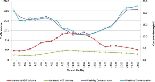
Based on vehicle registration data (both national and for Prince George’s County, Maryland), it was assumed that at least two-thirds of the HDT fleet on the Capital Beltway was diesel-fueled, and that emissions from these vehicles would contribute to nearby PM_2.5 concentrations. However, the data show an inverse variation between HDT traffic volumes and PM_2.5 concentrations at the SHA monitor—lower concentrations were recorded during periods with higher total truck volumes. This could be the effect of the daytime turbulence: the high HDT volumes are higher during the daytime when turbulence is also high.

To determine if there is a correlation between local traffic-related emissions and PM_2.5 concentrations at the monitoring site, analyses were conducted using only hours, firstly, when the wind was blowing from the roadway towards the monitor and, secondly, when HDT percentage in the traffic mix was higher (at nighttime hours). Additionally, the analysis examined the sensitivity of the monitored concentrations to the travel speeds. The analyses were conducted separately for each season to explore the impact of the season variation.

No significant correlation between the traffic-flow characteristics and monitored concentrations were found. An additional analysis of hourly concentrations for days with recorded PM_2.5 levels greater than the 35 μg/m³ 24-hr NAAQS did not reveal any direct relationship between traffic volumes and monitored concentrations.

Comparison of speciation results

Comparison of compounds in the collected PM_2.5 samples reveal that elemental carbon is higher at the SHA site than at the McMillan or HU-Beltsville sites (see Figure 12). Elemental (or black) and organic carbon are products of the incomplete combustion of fossil fuels or biofuels. According to the review of national inventories of elemental and organic carbon emissions, the prevalent source of black carbon is on-road diesel combustion (Chow et al., 2010). The gasoline-fueled engines exhaust elemental carbon (EC) primarily in cold temperatures before the engine has warmed up and generally in small amounts compared with diesel-fueled engines. As there are few (if any) cold engines traveling on the Capital Beltway near the SHA site, the higher levels of EC at the SHA site is therefore an indicator of higher impacts of emissions from diesel traffic, since this is the only continuous major source of EC in the vicinity of the monitor that operates on a continuous basis.

Figure 12. Comparison of species distribution between SHA, McMillan, and HU-Beltsville sites.

Organic carbon (OC) is generated from various types of combustion (residential heating, cooking, agricultural burning, forest fires, as well as on/off-road fuel combustion). It also results from photochemical reactions with the vehicle exhaust gases (NO_x and VOCs) in the atmosphere and decomposition of biological material (e.g., plant detritus and food wastes). Since the OC levels are similar at the McMillan Reservoir and HU-Beltsville site, the OC concentrations measured at these sites are likely to be of regional origin—generated by traffic in the region, other regional sources, and/or by secondary formation in the atmosphere.

A crustal matter comparison also shows slightly higher levels at the SHA site, which may indicate the presence of a major roadway in the vicinity. Part of this crustal matter could be resuspended road dust.

Nitrate, sulfate, and ammonium are secondary aerosols produced by photochemical reaction of combustion products. The dominant source of ammonium sulfate in the United States is sulfur dioxide (SO₂) from coal-fired power plants, whereas ammonium nitrate results from conversion of nitrogen oxides, which are produced by all combustion sources.

The “other” pollutants on Figure 12 are composed of the compounds that are not connected with nearby roadway traffic emissions.

Apportionment of the PM_2.5 mass concentrations at the SHA site

To attribute the compounds found on the sampling filters to emission sources, the samples collected during the monitoring period were analyzed for gravimetric mass, OC and elemental carbon (EC), nitrate, sulfate, several cations such as ammonium, sodium, and potassium, and trace elements by X-ray fluorescence spectroscopy. Additionally, individual quartz filters collected in a month were combined and extracted with a solvent. The solvent extracts were analyzed for over 100 organic compounds, including polycyclic aromatic hydrocarbons, hopanes, steranes, and alkanes, using a gas chromatograph–mass spectrometer. Monthly average ambient concentrations of all analytes were calculated, and 45 of the most chemically stable and consistently detected analytes were selected for use in source apportionment.

Apportionments were estimated using version 8 of the Chemical Mass Balance (CMB-8) receptor model (Fujita et al., 2007, pp. 721–740; EPA, 2004). The CMB-8 program finds the linear sum of products of source profile abundances and source contributions that best match the observed chemical composition of samples collected at a receptor site. The results provide an estimate of the amount of each measured parameter in individual ambient samples that was contributed by each source type represented by a profile, along with calculated uncertainty for the estimates. Since CMB-8 quantifies contributions from chemically distinct source types, rather than emissions from individual sources, emissions with similar chemical composition cannot be distinguished from each other and chemical species that are created or transformed during transport may not be correctly apportioned.

Source profiles were selected to represent major on-road source types: light-duty gasoline powered vehicle exhaust, heavy-duty diesel vehicle exhaust, brake wear, and tire wear. The vehicle exhaust profiles were composites of multiple measurements of cooled and diluted vehicle exhaust collected during the National Renewable Energy Laboratory, Department of Energy (NREL/DOE) Gas/Diesel PM Split project in Riverside, California (Fujita et al., 2007). Several composite profiles were used for both the gasoline and diesel source categories, to represent different fleet mixes and driving patterns. These profiles do not represent current diesel vehicle emissions control technology, which began to be implemented in trucks manufactured after 2006. Although this may contribute some additional uncertainty to the apportionment of EC and nitrate, the EPA’s MOVES2014 emission model estimates that in 2010 more than 80% of heavy-duty trucks were pre-2007 model year (EPA, 2014). The composite profiles for brake wear and tire wear were created at University of California Riverside’s CE-CERT (College of Engineering Center for Environmental Research & Technology) laboratory using specially designed simulators (Fitz et al., 2003). Source profiles for biogenic sources such as forest fires, residential wood burning, vegetative decay, and cooking were not included, since identification of these sources typically relies on polar organic species, which were not part of the ambient data set. Based on prior experience, it is not expected that biogenic sources would be substantial contributors to the average composition of roadside ambient aerosol at this site, which is near a major highway in an area cleared of vegetation and surrounded by residential and light industrial land use (see Figure 1).

The results of the apportionment indicated that, on an annual basis, approximately 12.5–17% of the sampled aerosol mass came from on-road sources (see Table 3 and Figures 13, 14, 15, and 16), which was a combination of gasoline and diesel exhausts and brake and tire wear. The crustal material percentage indicated in the table is based on the measured amounts of major soil elements (Al, Si, Fe, etc.) adjusted to their common oxide forms, since no local soil profile was available. The individual monthly total direct roadway contributions varied from 7% to 20% depending on the season—slightly lower in the summer (7–16%) because of larger contributions from organic aerosols. A portion of the ammonium nitrate and ammonium sulfate compounds found in the sampled PM_2.5 matter could also be attributed to on-road sources, but are more likely to be of regional origin. These compounds are present in large proportions in the air over the Northeast United States, and since they are secondary aerosol components produced by atmospheric chemical reactions, it is impossible to separate regional impacts from that of local traffic impacts using the CMB receptor model.

Table 3. Annual source apportionment of PM_2.5 mass concentrations

Year	PM2.5 Concentration (µg/m^3)	Gasoline Exhaust	Diesel Exhaust	Tire and Brake Wear	Ammonium Sulfate	Ammonium Nitrate	Crustal Matter (Unidentified)	Other Unidentified Source (Not Directly from Vehicles)	Total On-Road
2009	10,619	0.6 ± 1.3%	9.5 ± 1.5%	2.4 ± 0.1%	33.4 ± 1.1%	7.9 ± 0.2%	1.4%	45%	12.5%
2010	10,613	1.3 ± 1.6%	13.0 ± 2.3%	2.2 ± 0.1%	36.9 ± 1.5%	20.1 ± 0.8%	2%	24%	17%
2011	9712	1.5 ± 1.0%	9.0 ± 4.4%	2.1 ± 0.1%	31.4 ± 2.3%	13.3 ± 1.3%	1%	41%	13%
2012	9936	0.9 ± 0.6%	9.0 ± 1.0%	2.2 ± 0.1%	27.9 ± 0.8%	14.4 ± 0.4%	2%	44.%	12%

Notes: PM_2.5 source apportionment results for ICC site for 2009–2012 monitoring years are from DRI.

Figure 13. PM_2.5 apportionments at SHA site in 2009 by month.

Figure 14. PM_2.5 apportionments at SHA site in 2010 by month.

Figure 15. PM_2.5 apportionments at SHA site in 2011 by month.

Figure 16. PM_2.5 apportionments at SHA site in 2012 by month.

In addition, an AERMOD modeling study was conducted to compare the modeled and monitored impacts of the roadway traffic emissions. The study utilized an average hourly traffic data collected at the SHA ATR station and the Baltimore-Washington International (BWI) Airport meteorological data. The results of the analysis indicated that the highest contribution of the road emissions at the monitoring site would constitute approximately 12% of the highest measured concentration at the site. This is in agreement with the apportionment results.

Conclusion

The SHA monitoring program was set to research into the influence of the traffic emissions on the PM_2.5 concentrations close to the major roadways. The program utilized two PM_2.5 monitors, the E-BAM and the Super SASS, located about 150 m (500 feet) away from the Capital Beltway (I-95/I-495). The first unit was used for continuous monitoring and the second for speciation monitoring. Additional data collected included on-site meteorological observations, traffic information on Capital Beltway about 150 m away from the monitoring site, and continuous and speciation PM_2.5 data at the HU-Beltsville and McMillan Reservoir sites selected for comparison. A total of 29,647 hr (1234 days) of continuous PM_2.5 concentrations and 204 daily samples of speciation monitoring were collected during the 3½ yr of observations at the SHA monitoring site.

The analysis of continuous concentrations at the SHA site found no exceedances of the current 24-hr or then current annual PM_2.5 NAAQS. The 24-hr concentration comparable to the standard is 32.3 μg/m³ and the annual design concentration is 13.0 μg/m³.

Comparison with the PM_2.5 concentrations collected at HU-Beltsville and McMillan Reservoir sites showed that concentrations at the SHA site were consistently higher. The EC concentrations (a surrogate for diesel particulate matter) were also consistently higher at the SHA site. This difference would point to the singular major emission source near the SHA site—the Capital Beltway traffic. However, no direct correlation with traffic volumes (general or HDT) or speeds was found in the collected data. This result could indicate that impacts of traffic emissions are not immediately noticeable at the distance of 150 m (500 feet) from the roadway. The apportionment analysis revealed that about 12.5–17% (the average of 14.2%) of particulate material collected at the site could be attributed to the roadway sources. This result is supported by the results of the AERMOD modeling conducted for the site.

Acknowledgment

The program would not be possible without the vigilance and uninterrupted attention from our field engineers, Megan Berg and Nick Campanella from the URS construction services at the Intercounty Connector Project. The authors express their appreciation to Jeff Nichol, James O’Rourke, and other laboratory staff at RTI International for training and laboratory analyses.

Additional information

Notes on contributors

Helen Ginzburg

Helen Ginzburg is an air quality scientist and a principal professional associate and Xiaobo Liu is an environmental engineer at Parsons Brinckerhoff in New York.

Xiaobo Liu

Helen Ginzburg is an air quality scientist and a principal professional associate and Xiaobo Liu is an environmental engineer at Parsons Brinckerhoff in New York.

Michael Baker

Michael Baker is an environmental construction manager for URS Corporation on the Intercounty Connector Project in Maryland.

Robert Shreeve

Robert Shreeve is a deputy director at the Office of Environmental Design and Office of the Intercounty Connector at Maryland State Highway Administration in Baltimore.

R.K.M. Jayanty

R.K.M. Jayanty is a distinguished fellow at RTI International, Research Triangle Park, North Carolina.

David Campbell

David Campbell is an associate research scientist in the Division of Atmospheric Sciences and Barbara Zielinska is a research professor at the Desert Research Institute in Reno, NV.

Barbara Zielinska

David Campbell is an associate research scientist in the Division of Atmospheric Sciences and Barbara Zielinska is a research professor at the Desert Research Institute in Reno, NV.

References

- Baldauf, R., D. Heist, V. Isakov, S. Perry, G.S.W. Hagler, S. Kimbrough, R. Shores, K. Black, and L. Brixey. 2012. Air quality variability near a highway in a complex urban environment. Atmos. Environ. 64:169–178. doi:10.1016/j.atmosenv.2012.09.054
- Baldauf, R., E. Thoma, M. Hays, R. Shores, J. Kinsey, B. Gullett, S. Kimbrough, V. Isakov, T. Long, R. Snow, A. Khlystov, J. Weinstein, F.L. Chen, R. Seilaf, D. Olson, I. Gilmour, S.H. Cho, N. Watkins, P. Rowley, and J. Bang. 2008. Traffic and meteorological impacts on near-road air quality: Summary of methods and trends from the Raleigh near-road study. J. Air Waste Manage. Assoc. 58:865–878. doi:10.3155/1047-3289.58.7.865
- Baldauf, R., N. Watkins, D. Heist, C. Bailey, P. Rowley, and R. Shores. 2009. Near-road air quality monitoring: Factors affecting network design and interpretation of data. Air Qual. Atmos. Health 2:1–9. doi:10.1007/s11869-009-0028-0
- Black, K., V. Martinez, M. Gaber, R. Baldauf, E. Thoma, and D.L. Costa. 2009. Study design to evaluate mobile source emissions in the near-road environment. EM 2009(January):26–29.
- Chow, J., J.G. Watson, D.H. Lowenthal, L.A. Chen, and N. Motallebi. 2010. Black and organic carbon emission inventories: Review and application to California. J. Air Waste Manage. Assoc. 60:497–507. doi:10.3155/1047-3289.60.4.497
- Fitz, D.R., J.M. Chow, and B. Zielinska. 2003. Development of a Gas and Particulate Matter Organic Speciation Profile Data Base. Final report prepared for San Joaquin Valleywide Air Pollution Study Agency, Sacramento, CA: California Air Resources Board.
- Fujita, E.M., D.E. Campbell, W.P. Arnott, J.C. Chow, and B. Zielinska. 2007. Evaluations of the chemical mass balance method for determining contributions of gasoline and diesel exhaust to ambient carbonaceous aerosols. J. Air Waste Manage. Assoc. 57:721–740. doi:10.3155/1047-3289.57.6.721
- Fujita, E.M., D.E. Campbell, B. Zielinska, W.P. Arnott, and J.C. Chow. 2011. Concentrations of Air Toxics in Motor Vehicle-Dominated Microenvironments. Research Report 156. Boston, MA: Health Effects Institute.
- Fujita, E.M., B. Zielinska, D.E. Campbell, W.P. Arnott, J. Sagebiel, L. Reinhart, J.C. Chow, N. P.A. Gabele, W. Crews, R. Snow, N. Clark, S. Wayne, and D.R. Lawson. 2007. Variations in speciated emissions from spark-ignition and compression ignition motor vehicles in the California’s South Coast air basin. J. Air Waste Manage. Assoc. 57:705–720. doi:10.3155/1047-3289.57.6.705
- Ginzburg, H., G. Schattanek, D. Lowes-Hobson, D. Gill, S. Tarantino, and A. Kasprak. 2012. Nitrogen oxides (NOx) near road monitoring program as part of the operating certification renewal of the central artery/tunnel project in Boston, Massachusetts. Paper presented at the 105th Air and Waste Management Association Annual Conference and Exhibition 2012, ACE, San Antonio, Texas, June 19–22, 2012.
- Health Effects Institute Panel on the Health Effects of Traffic-Related Air Pollution. 2010. Traffic-Related Air Pollution: A Critical Review of the Literature on Emissions, Exposure, and Health Effects. Special Report 17. Boston, MA: Health Effects Institute.
- Homolya, J., and J. Rice. 1999. Particulate Matter (PM2.5) Speciation Guidance, Final Draft, Edition 1. Research Triangle Park, NC: U.S. Environmental Protection Agency.
- Karner, A.A., D.S. Eisinger, and D.A. Niemeier. 2010. Near roadway air quality: Synthesizing the findings from real-world data. Environ. Sci. Technol. 44:5334–5344. doi:10.1021/es100008x
- Kimbrough, S., R.C. Shores, and D.A. Whitaker. 2011. U.S. Environmental Protection Agency/Federal Highway Administration near road collaboration project: National near-road MSAT study. Paper presented at the Transportation Planning, Land Use, and Air Quality Conference, Transportation Research Board, San Antonio, Texas, May 9–11, 2011.
- Maryland State Highway Administration. 2014. Internet Traffic Monitoring System (I-TMS). http://shagbhisdadt.mdot.state.md.us/ITMS_Public/default.aspx (accessed 2009–2012).
- Met One Instruments, Inc. 2014a. E-BAM, a portable real time beta gauge traceable to USEPA requirements for automated PM2.5 and PM10 measurement. http://www.metone.com/documents/E-BAM_Datasheet_Rev_Aug09.pdf (accessed November 2008).
- Met One Instruments, Inc. 2014b. SASS/Super SASS speciation sampler to USEPA speciation requirements. http://www.metone.com/documents/SASS0301Particulate.pdf (accessed November 2008).
- Muruganandam, B.S, and S.M.S. Nagendra. 2011. Characterizing temporal variations of roadside PM10 and PM2.5 mass concentration. Paper presented at the Transportation Research Board’s 2011 Transportation Planning, Land Use and Air Quality Conference, San Antonio, Texas, May 9–11, 2011.
- NAVTEQ (Navigation Technology). 2014. Intelligent Transportation Infrastructure program. http://here.com/traffic ( formerly www.Traffic.com) ( accessed May–December 2009).
- Polidori, A., and P.M. Fine. 2012. Ambient Concentrations of Criteria and Air Toxic Pollutants in Close Proximity to a Freeway with Heavy-Duty Diesel Traffic. California: South Coast Air Quality Management District.
- Rowangould, G.M. 2013. A census of the US near-roadway population: Public health and environmental justice considerations. Transport. Res. D Transport Environ. 25:59–67. doi:10.1016/j.trd.2013.08.003
- Schattanek, G., H. Ginzburg, and J. Faeth. 2012. Air monitoring study to evaluate pollution effects of subway construction in New York City. In Proceedings of the 105th Air & Waste Management Association Annual Conference and Exhibition 2012, ACE, San Antonio, Texas, June 19–22, 2012. San Antonio, TX: Air & Waste Management Association.
- Thoma, E., R.C. Shores, V. Isakov, and R.W. Baldauf. 2008. Characterization of near-road pollutant gradients using path-integrated optical remote sensing. J. Air Waste Manage. Assoc. 58:879–890. doi:10.3155/1047-3289.58.7.879
- U.S. Environmental Protection Agency. 1998. 40 CFR part 58, Appendix E—Probe and Monitoring Path Siting Criteria for Ambient Air Quality Monitoring. http://www.gpo.gov/fdsys/granule/CFR-1998-title40-vol5/CFR-1998-title40-vol5-part58-appE/content-detail.html (accessed 2009).
- U.S. Environmental Protection Agency. 1999. 40 CFR part 50, Revisions to Reference Methods for the Determination of Fine Particulate Matter as PM2.5 in the Atmosphere. http://www.epa.gov/ttnamti1/files/cfr/met1.pdf (accessed 2009)
- U.S. Environmental Protection Agency. 2004. EPA-CMB8.2 Users Manual. EPA-452/R-04-011. http://www.epa.gov/scram001/models/receptor/EPA-CMB82Manual.pdf (accessed 2009).
- U.S. Environmental Protection Agency. 2006. 40 CFR parts 53 and 58, Revised Requirements for Designation of Reference and Equivalent Methods for PM2.5 and Ambient Surveillance for Particulate Matter; Final Rule. http://www.gpo.gov/fdsys/pkg/FR-2006-10-17/pdf/06-8478.pdf (accessed 2009).
- U.S. Environmental Protection Agency. 2011. 40 CFR part 50, Appendix L—Reference Method for the Determination of Fine Particulate Matter as PM2.5 in the Atmosphere. http://www.gpo.gov/fdsys/granule/CFR-2011-title40-vol2/CFR-2011-title40-vol2-part50-appL/content-detail.html (accessed 2009).
- U.S. Environmental Protection Agency. 2011. 40 CFR part 50, Appendix N—Interpretation of the National Ambient Air Quality Standards for PM2.5. http://www.gpo.gov/fdsys/granule/CFR-2011-title40-vol2/CFR-2011-title40-vol2-part50-appN (accessed 2009).
- U.S. Environmental Protection Agency. 2012. The National Ambient Air Quality Standards: Overview of the EPA’s Revisions to the Air Quality Standards for Particulate Pollution (Particulate Matter). http://www.epa.gov/pm/2012/decfsoverview.pdf (accessed December 2012).
- U.S. Environmental Protection Agency. 2014. Tools for MOVES. http://www.epa.gov/otaq/models/moves/tools.htm#fleet-2014 ( accessed 2014).
- Watson, J.G., J.C. Chow, L.W. Chen, D.H. Lowenthal, E.M. Fujita, H.D. Kuhns, D.A. Sodeman, D.E. Campbell, H. Moosmüller, D. Zhu, and N. Motallebi. 2011. Particulate emission factors for mobile fossil fuel and biomass combustion sources. Sci. Total Environ. 409:2384–96. doi:10.1016/j.scitotenv.2011.02.041
- Westerdahl, D., S. Fruin, T. Sax, P.M. Fine, and C. Sioutas. 2005. Mobile platform measurements of ultrafine particles and associated pollutant concentrations on freeways and residential streets in Los Angeles. Atmos. Environ. 39:3597–3610. doi:10.1016/j.atmosenv.2005.02.034
- Yoon, S.J. 2003. Measuring vehicle volumes and monitoring and modeling of PM2.5 concentrations in a travel center associated with a major urban interstate and interchange. In Proceedings of the Air & Waste Management Conference, San Diego, CA; June 22–26, 2003. San Antonio, TX: Air & Waste Management Association.
- Zhou, Y., and J.I. Levy. 2007. Factors influencing the spatial extent of mobile source air pollution impacts: A meta-analysis. BMC Public Health. 7:89. doi:10.1186/1471-2458-7-89
- Zhu, Y., W.C. Hinds, S. Kim, S. Shen, and C. Sioutas. 2002. Study of ultrafine particles near a major highway with heavy-duty diesel traffic. Atmos. Environ. 36:4323–4335. doi:10.1016/S1352-2310(02)00354-0