Aerosol particulate matter in the Baltimore metropolitan area: Temporal variation over a six-year period

Abstract

This study investigates the sources of fine particulate matter (aerodynamic diameter ≤2.5 μm; PM_2.5) composition for the Baltimore, Maryland, metropolitan area, covering a 6-year period (2008–2013). Data obtained from the U.S. Environmental Protection Agency (EPA) Air Quality System (AQS) were used for the identification of eight chemical speciation clusters (factors), which, as a percentage of the average concentration, were identified as secondary sulfate (31.9%), secondary nitrate (14.3%), gasoline (17.4%), diesel (10.1%), soil (4.0%), biomass burning (11%), marine aerosol (4.1%), and industrial processing (7.2%). The results show predominant influence from vehicle emissions transiting major highways I-695 and I-95 located in the vicinity of the sampling site. Strong influence on PM_2.5 mass from biomass burning was found in the first 2 years (2008–2009) due to particulate matter remnants from forest fire events in North Carolina and a strong contribution in 2013 that was due mainly to wood burning during winter. Sulfate, nitrate, soil, and marine aerosol fractions registered very low variability over the 6-year period analyzed. In addition, this study shows a significant reduction in particulate matter from industrial origins after a major industrial source in Baltimore shut down. The results obtained from Baltimore were compared with those from the Beltsville, Maryland, sampling station located 25 miles south of Baltimore for 2011 and 2012, where good agreement was found for most of the factors.

Implications: This paper presents the first long-term aerosol speciation analysis in a Mid-Atlantic United States metropolitan area, which is essential for the air quality management agencies in order to revise regulations and reduce human exposure to adverse air quality conditions. The results suggest that although a declining trend in the overall PM_2.5 was observed, no significant tendency was observed in the identified sources besides exceptional events such as the impact of wildfires on local air quality and downward contribution from industrial fraction of PM_2.5 after the Steel Mill at Sparrows Point closure in 2012.

Introduction

Air pollution is an important problem that requires serious attention because of its impact on human health and air quality policy (Pope, 1996; Landis et al., 2001; Kidwell and Ondov, 2004). According to the U.S. Environmental Protection Agency (EPA), fine particle pollution can cause harmful effects on the cardiovascular system and enhance heart attacks and strokes, as well as harmful respiratory effects, including asthma episodes (EPA, 2012). In order to attack this issue, the EPA has periodically reviewed the daily and hourly concentrations that constitute an excess of regulatory acceptable levels of PM_2.5 (particulate matter with aerodynamic diameter less than or equal to 2.5 μm). For instance, in 2012, the annual PM_2.5 standard was set to 12 µg/m³ and the 24-hr average standard to 35 µg/m³ (EPA, 2012). Defining the sources of ambient particulate matter has become progressively more important as the regulations intensify and focus mostly on PM_2.5 emissions. However, although local sources can be supervised and subjected to local control regulations, the fraction of particulate matter that has been transported into the region cannot easily be assessed or controlled (Prospero, 1999; EPA, 2003a; Singh et al., 2009). Therefore, the estimation of particulate matter sources in a particular region (source apportionment) is essential for decision makers when evaluating agreement with new standards.

The characterization of PM components, their precursors, atmospheric transport, and source categories that affect the particle loading in a region is a crucial step for understanding source-receptor relationships and the factors that affect PM at a given site. The U.S. Supersites Program was created to establish and test new methods for monitoring particles and their aerosol initiators. Many of these methods have been included in components of the State and Local Air Monitoring System (SLAMS) such as the Speciation Trends Network (STN) (Chu et al., 2004; Flanagan et al., 2006), Interagency Monitoring of Protected Visual Environments (IMPROVE) network 2.0 (Watson et al., 2008), and the Southeastern Aerosol Research and Characterization (SEARCH) network (Hansen et al., 2006). Combined with receptor models, these methods are used to identify sources, analyze properties of the pollutants at the receptor site, and to estimate their contributions.

Receptor models have been used widely not only for the identification of major sources of particulate matter, but also to establish emission reducing policies to certain standards of PM₁₀ (particulate matter with aerodynamic diameter less than or equal to 10 μm), PM_2.5, and ozone (O₃). Consequently, different chemical markers, such as trace elements in industrial emissions and lead (Pb) in gasoline engine exhaust have been substantially reduced or virtually eliminated (Watson et al., 2008). The central principle of most receptor models relies on the assumption that mass is conserved and a mass balance can be used to recognize and apportion sources of PM (Hopke, 1991). Using this principle, receptor-modeling methods that incorporate the concentrations of aerosol species at a receptor site have been demonstrated to be effective in determining aerosol sources (Gordon, 1988; Xie et al., 1999). Positive matrix factorization (PMF; see Model Overview) is a mathematical tool that requires simplifying assumptions to provide insight into the actual particulate matter sources. PMF has been used extensively in source apportionment studies, since it offers a practical alternative in the absence of a local source inventory, despite the assumptions and the level of accuracy.

The Maryland Department of the Environment (MDE) has sampled aerosol particles and trace gases for more than a decade in Baltimore. However, the knowledge of the major sources of these particles in this region is not well known and a long-term speciated analysis has not been reported. Consequently, the aim of this study was to identify the main sources of particulate air pollution in the Baltimore metro area through the application of the PMF model on species measured with a 24-hr resolution acquired from 2008 to 2013. This identification of sources is of great importance, since traffic on the highways, industries, residential cooking, and heating in general are significant contributors to the particle matter loading in the Baltimore-Washington corridor (Chen et al., 2002). This apportionment of the pollutants on a long-temporal scale offers not only the identification of main sources in the region, but also the variation of the sources over the studied period, producing the first longitudinal PM_2.5 classification inventory for the air quality management agencies.

Sample Collection and Analytical Method

The 24-hr PM_2.5 filter samples used for this study were collected every 3 days at the Maryland Department of the Environment Essex air quality monitoring station (39.3107°N, 76.4744°W) located 10 miles northeast of downtown Baltimore (Figure 1). The Speciation Trends Network (STN) procedure collects PM_2.5 particles on Teflon, nylon, and quartz filters using a modular, cyclone-based sampler with specific flow design to fulfill the EPA sampling requirements (EPA, 1997). Different methods, such as gravimetric analysis, ion chromatography (IC), X-ray fluorescence (XFR), and thermal optical reflectance, are used to analyze the filters in order to obtain mass concentrations of trace elements with atomic number (Z) from 11 to 82 (Na–Pb); Na⁺, K⁺, NH₄⁺, NO₃⁻, and SO₄²⁻ ions; elemental and organic carbon (EC and OC, respectively); as well as the coefficient of absorption. Carbonaceous loadings, such as OC, EC, and carbonate materials, account for a considerable fraction of PM_2.5 mass in most atmospheric environments. EC is more resistant to high temperatures and absorbs more light than OC, so that these components are often separated by optical and thermal methods. Watson et al. (2005) indicated that different carbon measurement methods report different EC abundances for the same samples by up to an order of magnitude. The IMPROVE network has used the thermal/optical reflectance method since its beginning (Chow et al., 1993), whereas the Speciation Trends Network (STN) started using a modified IMPROVE carbon sampler (i.e., URG 3000N carbon sampler; URG Corp., Chapel Hill, NC) after 2007 in order to apply the thermal/optical reflectance method on the sampled particles (Chow et al., 2007). Therefore, the analytical procedure used by the present study was that of IMPROVE.

Figure 1. Map of Baltimore area and sampling sites.

Model Overview

EPA PMF (Positive Matrix Factorization) 5.0 is a software package distributed by the EPA Office of Research and Development (Norris et al., 2014). This multivariate factor analysis tool, based on the Multilinear Engine (ME-2), resolves speciated sample data into source contributions and source profiles (Paatero and Tapper, 1994; Paatero, 1997). The great advantage of PMF compared with other analysis methods relies on the physical constraint that there cannot be negative species concentrations and, therefore, only positive factor contributions are yielded (Paatero and Tapper, 1993, 1994). Analytic techniques, including multivariate factors, have been shown to be sensitive to variables with a high proportion of data less than the minimum detectable limit (MDL). Therefore, the uncertainty for each measured concentration in the analysis is based on the proportion of each individual species’ measurements that are greater than the MDL. By using this method, species that are constantly below the detection limit are filtered, since they constitute most of the noise and have a significant impact on the final result of a PMF analysis. Three criteria were used in this work to evaluate the validity of each variable. If the signal to noise ratio value was greater than 2, then the variable was considered “good.” If the value was between 0.2 and 2, the variable was considered “weak,” and the variable was considered “bad” if it was less than 0.2. (Paatero and Hopke, 2003). Uncertainties for “good” variables were either the MDL or the root mean square average of 10% of the measured concentration. “Weak” variables had uncertainties that were either the MDL or the root mean square average of 3 times the measured concentration and 3 times the MDL, whichever was larger. This weighting method minimizes the impact of those species on the fitting of the model. Species determined by the above criteria to be “bad” were not used in this analysis. The extra modeling uncertainty for this study was 10%, and the PM_2.5 data were considered as a total variable. The total variable is selected to scale the output of ME-2 back into its original units. The base model consisted of the best of 20 runs (weighted by least squares) for eight factors with random seed.

Data

Twelve years (2001–2013) of PM_2.5 data collected every 3 days were reported for the Essex air quality monitoring station. However, this study focuses on the period between 2008 and 2013, since the complete fractions of carbonaceous aerosol (OC1, OC2, OC3, OC4, EC1, EC2, and EC3) were available in those years. The analytical carbonaceous fractions are indispensable for identifying major combustion sources of interest, such as gasoline and diesel. A total of 554 days were considered in this analysis. Figure 2 shows the time series of PM_2.5 data from the period studied. The PM_2.5 concentrations registered in Baltimore have been fairly constant during the entire period, with few unhealthy Air Quality Index (AQI) incidents recorded (EPA, 2003b). The reduction of PM_2.5 concentrations over a 13-year period is discussed in the next section. Samples collected during holiday events (e.g., Fourth of July and New Year’s Day) were excluded; PM_2.5 concentrations on these days are challenging in a multivariate analysis because firework displays introduce a large bias in the source apportionment (Brown et al., 2007; Rizzo and Scheff, 2007). As described in Table 1, the major contributing species used in this analysis include sulfate, nitrate, organic and elemental carbon, aluminum, sodium, potassium, zinc, and silicon. Nitrogen oxide (NO_x) and hydrocarbon concentrations obtained from the Photochemical Assessment Monitoring Stations (PAMS) network also sampled in Essex, Maryland (MD), were used in this study to evaluate trends and to discuss the role of organic compounds in the gasoline factor. Moreover, PM_2.5 speciated data collected at the MDE’s Howard University Beltsville Research Campus (HUBRC; 39.05°N, 76.87°W; Figure 1), was used to compare the overall performance of the model and to observe differences between urban and semirural particulate sources.

Table 1. Summary of statistics of PM_2.5 (ng/m³) chemical species concentrations sampled at MDE Baltimore station (Essex) from 2008 to 2013

Species	S/N	Maximum	Median	Mean	SD
Arsenic	1.5	32.2	0.4	0.9	1.9
Aluminum	3.3	361.0	11.4	22.0	35.7
Bromine	4.7	95.7	2.9	3.9	5.2
Calcium	11.1	547.0	24.0	31.2	34.6
Chromium	3.0	151.0	1.0	2.3	7.7
Copper	5.8	98.7	2.0	3.0	5.8
Chlorine	11.4	745.0	7.2	22.5	67.0
Iron	12.5	708.0	57.3	74.2	66.6
Lead	1.4	36.8	1.3	2.4	3.5
Manganese	2.3	14.5	1.1	1.5	1.8
Nickel	2.2	9.5	0.5	0.9	1.1
Magnesium	2.6	337.0	0.0	5.4	20.5
Titanium	1.8	28.9	0.6	2.0	3.6
Vanadium	1.3	11.5	0.4	1.2	1.8
Silicon	8.5	765.0	37.3	52.7	68.1
Zinc	8.4	73.1	7.8	10.0	8.5
Sulfur	13.0	5370.0	811.5	966.8	634.7
Potassium	13.0	3680.0	55.7	101.9	204.5
Sodium	4.8	812.0	27.5	53.1	84.7
Total nitrate	13.0	8170.0	830.0	1365.9	1307.9
OC1	9.0	2280.0	171.0	271.5	301.6
OC2	9.0	2690.0	551.0	619.9	324.4
OC3	9.0	3360.0	502.0	617.9	409.0
OC4	9.0	1920.0	380.0	471.5	285.5
EC1	9.0	5610.0	1010.0	1144.2	709.3
EC2	8.3	166.0	41.7	46.1	23.3
EC3	1.2	18.2	0.2	0.2	1.4
Sulfate	13.1	14800.0	2320.0	2758.5	1817.1

Figure 2. PM_2.5 total concentration from 24-hr filter time series for Maryland Department of the Environment Baltimore station (Essex) for 2008–2013.

Results and Discussion

Selecting the optimal number of factors is a decisive step in the PMF model (Paatero, 1993). Mathematical diagnostics for the best performance of model fit can be used as criteria to define the ideal number of factors. However, the criteria for this selection solution should be determined by the interpretation of the model results, and in most cases, some factors are composed of mixtures of different sources. Four to nine factors were considered in this study. Nevertheless, an eight-factor solution produced the most interpretable and reproducible results for the data collected during the 6-year period, performing annual analysis to identify seasonal variations. The PM_2.5 reconstructed by the model agrees well with the observed PM_2.5 at the Essex sampling station for all the years. On average, R² = 0.96 ± 0.02 with 0.51 ± 0.24 intercept and slope of 0.93 ± 0.02. In order to identify the sources, the resolved source profiles from the PMF modeling were compared and analyzed using key indicator species reported from previous source apportionment studies (Lee et al., 1999; Chueinta et al., 2000; Ramadan et al., 2000; Song et al., 2001; Watson et al., 2001; Qin et al., 2002; Kim et al., 2003; Chow et al., 2004; EPA, 2004; Almeida et al., 2005; He et al., 2006; Yuan et al., 2006; Gildemeister et al., 2007; Bullock et al., 2008; Yatkin and Bayram, 2008; Callén et al., 2009; Srimuruganandam and Shiva, 2012). The eight factors were identified as gasoline, secondary sulfates, diesel, secondary nitrates, marine aerosols, biomass burning, soil, and industrial processing.

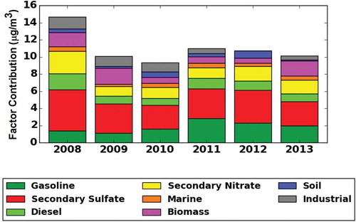
The seasonal variability of the factor contributions in PM_2.5 mass (μg/m³) is presented in Figure 3, where the seasonal trends are also shown. Table 2 provides a summary of the average mass contribution data for the analyzed period. Figure 4 shows the PMF source factor mass and composition profiles of PM_2.5 for each year from 2008 to 2013. Factor 1 was identified as gasoline, emitted mainly from motor vehicles, as the profiles are dominated by species related to gasoline combustion such as S, SO₄⁻², NO₃⁻, OC1, OC2, OC3, OC4, EC1, and EC2, with higher abundance in OC2 and OC3 (Kim and Hopke, 2004; Brown et al., 2007). The traffic monitoring system from the State Highway Administration of Maryland (SHA) reported that the annual average daily traffic (AADT) of vehicles (no trucks) measured on the I-695 by the roads MD-150 and MD-702 (which is the closest traffic counter point to the sampling site) was on average 60,126 during the 6-year period (http://www.roads.maryland.gov). Moreover, according to Maryland Transport Authority (MDTA), the daily number of vehicles (no trucks) transiting the I-95 Fort McHenry Tunnel (toll road) was on average 80,011 during the 6-year period (http://www.mdta.maryland.gov). The gasoline factor contribution to PM_2.5 mass, in μg/m³ (percentage), varied during the 4 years starting at 1.4 (9.4%) in 2008, 1.1 (11.2%) in 2009, and 1.6 (17.1%) in 2010. In 2011, this factor reached a peak with a contribution of 2.8 (25.7%), followed by a small decrease in the next years: 2.3 (21.4%) in 2012 and 2.0 (19.6%) 2013.

Table 2. Average seasonal factor contribution (μg/m³)

	Winter			Spring			Summer			Autumn
Factor	Mean	SE	%	Mean	SE	%	Mean	SE	%	Mean	SE	%
Gasoline	1.7	0.2	13.6	1.6	0.1	15.6	2.1	0.1	15.8	2.4	0.2	24.6
Secondary Sulfate	2.4	0.2	17.7	3.2	0.2	31.7	6.9	0.4	53.8	2.3	0.2	24.5
Diesel	2.1	0.2	14.6	0.8	0.1	8.2	0.9	0.1	6.6	0.9	0.1	9.1
Secondary Nitrate	3.5	0.2	28.8	1.6	0.1	15.7	0.2	0.1	1.6	1.1	0.1	11.1
Marine	0.4	0.1	3.3	0.7	0.1	6.8	0.3	0.0	2.2	0.4	0.1	4.3
Biomass	2.3	0.3	17.2	0.8	0.1	7.7	1.3	0.2	9.6	1.4	0.2	11.7
Soil	0.2	0.1	1.6	0.8	0.1	7.1	0.7	0.1	4.1	0.3	0.0	3.4
Industrial	0.7	0.1	5.5	0.7	0.1	7.3	0.8	0.1	6.5	1.0	0.1	9.8

Notes: SE = standard error; % = source contribution to PM_2.5.

Figure 3. Time series of positive matrix factorization (PMF) factor strengths for PM_2.5 24-hr filters collected at MDE Baltimore station (Essex) for 2008–2013.

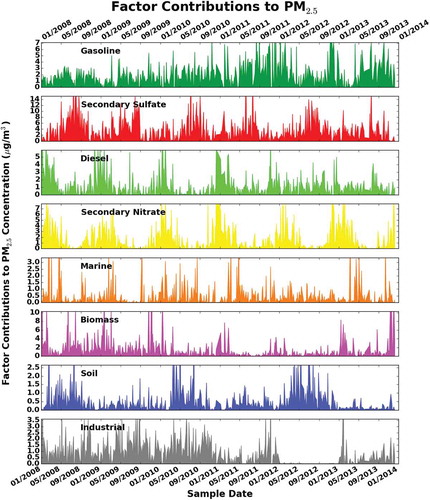
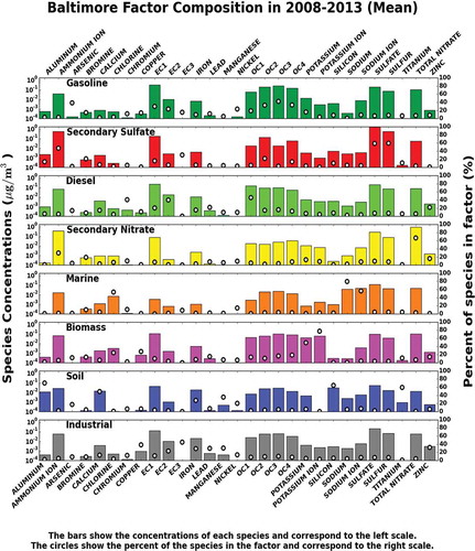
Figure 4. PMF factor profiles for samples collected at MDE Baltimore station (Essex) from 2008 to 2013.

The average contribution to PM_2.5 from this source and its standard deviation for the studied period is 1.9 ± 0.6 μg/m³ (17.4 ± 6.3%). Seasonally, this factor does not follow any pattern. The average contribution of this source was 20% higher on weekdays than on weekends, which is in agreement with the traffic volume on weekdays reported by SHA and MDTA.

Factor 2 is largely dominated by SO₄⁻², S, and NH₄⁺ and is the major contributor of the observed mass for all years. This factor was identified as secondary sulfates. Sulfate particles in the region are essentially formed by photochemical oxidation of sulfur dioxide, especially in the summer when solar radiation and the ambient temperature are relatively high (Seinfeld and Pandis, 1998). High relative humidity (RH) would enhance the dry conversion processes (Yao et al., 2003), corresponding to higher sulfate concentrations in summer than in other seasons (Figure 3). In addition, transport of sulfur and emissions from the heavily industrialized Ohio River Valley might influence the increase of the sulfate levels (Ogulei et al., 2005). The source contribution from this factor in the summer is 3 times greater than in winter (Table 2). Although the percent contribution from secondary sulfates to PM_2.5 total mass stayed relatively constant (31.8 ± 2.2%), the actual concentrations were different (3.5 ± 0.7 μg/m³), as shown in Figure 5.

Figure 5. Composition of PM_2.5 factor strengths from PMF modeling for MDE Baltimore station (Essex).

Factor 3, dominated by high concentrations of EC2, EC1, EC3 and OC1, OC2, OC3, OC4 along with iron, lead, and nickel, was interpreted as diesel emissions. The ratios of EC (EC1+EC2+EC3) to OC (OC1+OC2+OC3+OC4) in the diesel factor were on average 30% higher than those in the gasoline and were also used as criteria for the factor identification. Heavy diesel traffic comprising trucks and buses is responsible for most of the diesel contribution in the region (Shah et al., 2004; Ogulei et al., 2006). The AADT for trucks (classified as single and combined units from 2 to 7 or more axles) on the I-695 by the roads MD-150 and MD-702 and the daily number of trucks counted at the I-95 Fort McHenry Tunnel (toll road) were on average 8200 and 41,403, respectively, for the 6-year period. In addition, the factor might be influenced by ships’ emissions in the Port of Baltimore, due to the port’s close proximity to the air quality monitoring station. According to the Maryland Port Authority, approximately 2000 ships per year transit through the Port of Baltimore. The average diesel contribution to PM_2.5 for the 6 years was 1.1 ± 0.4 μg/m³ (10.1 ± 1.6%). The contribution of the diesel factor is 9% higher on weekdays than on weekends and peaks during the winter months. In addition to heavy diesel vehicles, this factor might be influenced by local incomplete combustion of materials such as wood used for heating during winter seasons.

Factor 4 is characterized by high nitrate and ammonium concentrations. Nitrate (NO₃⁻) is formed primarily from atmospheric processing of NO_x (NO_x = NO + NO₂) and emitted mainly by traffic and energy plants. According to Ogulei et al. (2005), nitrate loads in the Baltimore region can be formed during the transport of NO_x from industrial and urban surrounding areas, such as Pennsylvania and Virginia, as well as processing of NO_x emissions from traffic on highways I-695 and I-95. The contribution to PM_2.5 from nitrate sources is constant over the 6 years: 1.6 ± 0.5 μg/m³ (14.3 ± 2.9%). The influence of secondary nitrate is clearly seen in a pattern dominated by winter peaks (Figure 3).

High loadings of sodium and chlorine in factor 5 suggest the presence of aged sea salt or marine aerosol (Zhuang et al., 1999). This source can be explained by the atmospheric circulation at the sampling site, which is less than 3 miles from the Chesapeake Bay and is affected by the bay breeze. Moreover, rock salt (NaCl) usually spread during the winter enhances the marine aerosols factor during this season (Table 2). The average contribution and its standard deviation 0.4 ± 0.1 μg/m³ (4.1 ± 0.8%) to total PM_2.5 mass indicate a very constant impact over the 6 years from this source.

Factor 6 was identified as biomass burning due to the high presence of species such as OC1, EC1, and elemental potassium (K) (Brown et al., 2007; Karanasiou et al., 2009; Wang and Hopke, 2013). Potassium ion (K⁺) was included in the overall analysis. However, the biomass identification was based solely in K, since K⁺, as indicated by different studies, is not a good tracer for biomass burning due to its multiple sources (Zhang et al., 2010; Cheng et al., 2013). This factor accounts for sources such as residential fuel wood burning, wildfires, prescribed burning, open burning, and burning of agricultural and other biomass waste. The contributions from this source to PM_2.5, in μg/m³ (percentage), are 1.6 (11.3%) for 2008, 1.8 (18.0%) for 2009, 0.7 (7.3%) and 0.8 (7.0%) for 2010 and 2011, respectively, 0.6 (5.4%) for 2012, and 1.7 (17.2%) for 2013. The average contribution for the entire period was 1.2 ± 0.5 μg/m³ (11.0 ± 4.0%). The seasonal average mass contribution (Figure 3) shows peaks from this factor during summers of 2008, 2009, and 2013 when large fires occurred in the East Coast, as well as contributions in winters that are associated mainly with local heating.

High loadings of Al, Ca, Mg, Cu, Ti, and Fe were the key species used to identify factor 7 as local soil with a total average contributions of 0.4 ± 0.2 μg/m³ (4.0 ± 2.7%). The main sources of soil in the region comprise construction sites, wind-blown dust, and unpaved road dust.

In factor 8, trace metal elements such as Cr, Fe, Ni, and Mn were found at high concentrations and attributed to industrial processing sources. The contribution to PM_2.5 total mass in μg/m³ (percentage) from this source varied over the 6 years, with contributions of 1.4 (9.4%) in 2008, 1.2 (11.7%) in 2009, 1.1 (11.9%) in 2010, and 0.6 (5.5%) in 2011, reaching a minimum in 2012 with 0.1 (0.2%) and 0.4 (4.5%) in 2013. The average contribution for the 6 years to PM_2.5 was 0.8 ± 0.5 μg/m³ (7.2 ± 4.9%). The contribution of this factor was 21% higher on weekdays than on weekends, mostly due to the industrial operations on regular business hours. In this factor, no particular seasonal trend was observed.

Pollution roses obtained for each factor, for the 6-year period, using meteorological and PM_2.5 data collected at the Essex monitoring site were generated to observe the wind influence at the sampling site. Pollution roses are presented in Supplementary Material. The wind trends are similar for most of the factors, with major influence from the northwest during the study period. This suggests that in addition to pollution generated in Baltimore, the site is highly affected by nearby northwest cities such as White Marsh, Towson, Carney, and Parkville, MD (Figure 1).

Previous source apportionment studies centered on locations near Baltimore have shown similar results. Secondary sulfate, secondary nitrate, and carbonaceous loadings account for the majority of the total contribution to PM_2.5. Chen et al. (2002) ran a six-factor model covering a period of 2 years (1999–2001) using data from a suburban station at Fort Meade, MD, located in the middle of the Baltimore-Washington corridor. Sulfate, nitrate, ammonium, and carbonaceous material constituted more than 90% of the PM_2.5 mass sampled in Fort Meade. Ogulei et al. (2005) recognized nine major sources of PM_2.5 over a 9-month period (19 March through 26 November 2002); measurements for this study were made at the Ponca Street, Baltimore, supersite. The sources identified and the mass allocations by resolved source were oil-fired power plant (2%), spark-ignition emissions (26%), secondary nitrate (23%), aged sea salt (1%), steel plant (12%), incinerator (9%), coal-fired power plant (3%), secondary sulfate (23%), and diesel emissions (1%). Moreover, a 12-factor model was resolved for a 6-day period (July 6, 7, 8, 28, and 19, as well as August 21, 2002) from measurements made at Ponca Street where the 12 identified factors and their apportioned mass were oil-fired power plant (2.85%), secondary nitrate I (5.23%), local gasoline traffic (8.11%), coal-fired power plant (10.34%), secondary nitrate II (13.37%), secondary sulfate (14.68%), diesel emissions/bus maintenance (1.87%), Quebec wildfire episode (30.86%), nucleation (0.88%), incinerator (7.90%), airborne soil/roadway dust (3.47%), and steel plant (1.87%) (Ogulei et al., 2006).

The gasoline factor peak registered in 2011 was initially analyzed by the counts of vehicles transiting the major highways near the sampling site. According to the SHA’s traffic monitoring system, the AADT in 2011 increased by only 0.4% compared with the AADT of the previous year. This indicates that the increase in the gasoline factor was not necessarily caused by increased traffic. However, the speed of traffic on the highways could have a strong influence on the gasoline factor. The OC/EC ratios depend not only on the engine manufacturer, model, year, and size, but also on the operation mode. Most of the vehicular emissions are dominated by OC at low vehicle speed, whereas they are dominated by EC at higher constant vehicle speeds (Shah et al., 2004). Therefore, diesel vehicles running at low speeds can have a contribution in the gasoline factor (Wang and Hopke, 2013). According to the carbonaceous data from the resolved gasoline factor, the ratios of OC/EC were consistent throughout the entire period (2.11 ± 0.15). The average correlation between OC and EC was 0.84 ± 0.03 for the 6-year period, suggesting that OC is mostly generated by combustion sources (Chen et al., 2002), with no particular increase in 2011.

The increase recorded by the gasoline factor in 2011 is also unexpected in light of the emission inventories and measurements, which demonstrate that gasoline precursors such as NO_x, CO (carbon monoxide), and VOCs (volatile organic compounds) have been reduced in the last 20 years (Parrish et al., 2002; Parrish, 2006; Kim et al., 2009; Butler et al., 2011; Pusede and Cohen, 2012; Russell et al., 2010, 2011). According to the EPA National Emissions Inventory (NEI) Air Pollutant Emissions Trends Data (http://www.epa.gov/ttn/chief/trends/index.html), the total emissions of NO_x, CO, and VOCs report reductions of 51%, 64%, and 48%, respectively, in the United States from 1970 to 2013. Limits on these pollutants imposed by the EPA under the Clean Air Act for on-road and nonroad sources as well as industrial emissions in order to meet and maintain the National Ambient Air Quality Standards (NAAQS) have been responsible for these reductions. In particular, the Clean Air Interstate Rule (CAIR), the Acid Rain Program (ARP), and the NO_x State Implementation Plan (SIP) call for the Mid-Atlantic States are programs developed by EPA in order to reduce emissions of SO₂ (sulfur dioxide) and NO_x by power plants in the region (EPA, 2005; Godowitch et al., 2008). Therefore, in order to examine the increase of gasoline factor in Baltimore for 2011, the NO_x data trend was observed along with the average PM_2.5. In Baltimore, the PM_2.5 concentrations have declined ~5 µg/m³ in the last 13 years due to the imposed regulations (Figure 6). Yearly average NO_x concentrations from 2001 to 2013 also show a declining trend (Figure 6). However, the data display a small increase in NO_x from 2009 to 2011 that could be correlated to the rise of the gasoline factor during the same period. Particularly, NO_x data follow the same pattern as that of gasoline for 5 out of the 6 years considered in this analysis, that is, from 2009 to 2013. The ambient temperature at the sampling station in 2011 registered the second warmest summer and the coldest winter during the 6-year period, which could favor NO_x aerosol formation. Moreover, the ultraviolet (UV) index, reported by the National Weather Service (ftp://ftp.cpc.ncep.noaa.gov/long/uv/cities), denotes that during 2011 more days were classified under very high clear-sky UV index than any of the other years in the study, favoring photochemistry for NO_x production.

Figure 6. Yearly NO_x and PM_2.5 average collected at MDE Baltimore station (Essex). Error bars correspond to 95% confidence intervals.

The role of VOCs in the gasoline factor was also studied by evaluating carbonaceous molecular data obtained from the PAMS network also sampled in Essex from 2009 to 2013. In total, 138 samples per year with 59 species containing saturated (alkanes), unsaturated (n-alkenes), and aromatic (arenes) hydrocarbons were evaluated. The total average of nonmethane organic carbon (NMOC), a measure of total organic carbon, except for CH₄ (Mitra et al., 2001), registered a slightly larger contribution in 2011 (Figure 7). The n-alkanes concentrations are constant throughout the 5 years (Figure 7). Nevertheless, the n-alkanes reported by PAMS account only for low-carbon molecules C₆–C₁₀ (n-hexane, n-heptane, n-octane, n-nonane, n-decane) in contrast to high-carbon molecules (C₁₅–C₂₆) usually used as markers for VOCs from gasoline (Nekhoroshev et al., 2009). According to Chin and Batterman (2012), toluene, benzene, n-heptane, cyclohexane, and methylcyclohexane were the predominant vapor compounds detected in gasoline at 20 and 40 °C. However, no particular trend was found in those compounds as reported by PAMS. Although the influence of biogenic organic carbon is believed to be minor due to the urban location of the sampling site, the organic carbon markers used to identify the gasoline factor can also have a contribution from natural biogenic VOCs. The biogenic organic compound isoprene reported by PAMS was mostly uniform during the study period with a maximum concentration during 2010 (Figure 7). According to the temperature records, this maximum in isoprene was strongly enhanced by the high temperatures during the summer of 2010, as isoprene emissions are known to increase with temperature (Rasulov et al., 2010).

Figure 7. Yearly NO_x, NMOC, n-alkanes, and isoprene average collected at MDE Baltimore station (Essex).

Aside from the rise of NO_x and NMOC registered in 2011, the analysis does not yield strong evidence for the gasoline increase. This uncertainty leads to the hypothesis that the increase recorded in the gasoline factor in 2011 could be due to the mathematical model performance, in which the model may have allocated mass from a different source into the gasoline factor. In particular, mass from the industrial factor may have been used, since a considerable decline in the industrial factor was registered in the same year.

The high biomass contribution obtained in 2008 is attributed to the wildfire events in the month of June in North Carolina, where two large forest fires took place. The fires were considered significant and exceptional due to their large size, especially since dense smoke yielded air quality exceedances in various states, including Maryland (Delgado et al., 2014). In addition, smoke reported in Alaska and British Columbia, Canada, in 2009 spread across the northern United States, arriving in the Mid-Atlantic coast in early August, evidenced by back-trajectories and lidar measurements at UMBC (http://alg.umbc.edu/usaq/archives/003445.html). This factor also shows high contribution due to wood burning during winter months, especially January and February, where heavy snowstorms took place for several days in the region. Likewise, the sudden biomass increase in 2013 is attributed to two potential sources. First, wood burning due to the early start of the winter with colder temperatures than usual occurred for the last months of the year. Second, a derailment of a freight train and further fire consumption of numerous rail cars that took place in Rosedale, MD, 2.45 miles west from the sampling site, and within the range of the most predominant wind direction towards the site during that week. Finally, the significant decrease in the industrial factor is strongly related to the closure of the Sparrows Point Steel Mill, the largest steel mill in Maryland, due to bankruptcy in May 2012. This factor reached its lowest value that year with a 0.2% contribution.

In addition to the analysis for the urban site in Baltimore, speciated data from a semiurban station in Beltsville, MD (HUBRC), located in the Baltimore-Washington corridor, 25 miles south from Baltimore, were also analyzed in this study to compare the overall result of the model and to identify local pollution sources. The model was set to find an eight-factor solution with model characteristics similar to the Baltimore analysis. The identification of factors for the Beltsville site was carried out using same marker species employed in the Baltimore analysis. Figure 8 shows the contribution from sources to PM_2.5 total mass in 2011 and 2012 at each site. The PMF results from this site for 2011 and 2012 are in agreement with the modeling performed in Baltimore. Overall, the results follow a similar composition, having secondary sulfates, gasoline, and secondary nitrates as the higher contributors to PM_2.5 mass. The comparison of gasoline contributions for both sites in 2011 was 10% higher in Baltimore than in Beltsville. The increase registered in Baltimore may have been caused by local sources. For the other factors, the model showed uniformities and minimal differences based on geographic variances and locations of sources around the sampling sites.

Figure 8. Source contribution (%) comparison between PMF results for Baltimore and Beltsville, MD.

Besides the external biomass events registered in 2008 and 2009, and the decline in industrial emissions, this study indicates that although the overall PM_2.5 decreased ~3 µg/m³ during the 6-year period, no significant trend was found in the fractionation of species leading to particulate matter in Baltimore. Biogenic aerosols emitted mainly by vegetation, plant debris, pollen, and fungal spores among others as primary and secondary organic aerosols (SOAs) in the region are not directly quantified in this apportionment due to the lack of specific VOC markers in the available data. However, the carbonaceous components from biogenic sources, and SOAs in general, are contained within the identified factors obtained by the factorization of the total fractions of OC. Figure 4 shows that besides gasoline, biomass, and diesel, known for high amounts of OC, all the remaining factors found in this work have contributions from OC, in which primary and secondary organic aerosols can be masked. The contribution from the dense vegetation surrounding Baltimore and its impact on PM_2.5 concentrations by primary biogenic organics is possible through analysis such as gas chromatography and mass spectroscopy to retrieve known carbon markers, such as nanocosane, hentriacontane, tritriacontane, and alkanoic acids (Heo et al., 2013). Unfortunately, these techniques have not been implemented in Baltimore. The only indicator of biogenic reported by PAMS is isoprene (http://www.epa.gov/ttnamti1/pamsmain.html), which in Baltimore presented a constant contribution from 2009 to 2013, except for a 45% increase in 2011 due to high temperatures registered in that summer. Nevertheless, this increase was not reflected in a particular source, which suggests that biogenic carbonaceous seem to be affecting all sources similarly.

Summary and Conclusion

Six years of speciated data (2008–2013) collected on a 24-hr basis as part of the STN program at Essex, MD, were used to investigate the long-term contribution from different sources to PM_2.5 total mass in Baltimore, MD. The modeled results were consistent with known sources and their locations. Eight factors were identified as follows: sulfate-rich secondary aerosol (31.9%), nitrate-rich secondary aerosol (14.3%), gasoline (17.4%), diesel (10.1%), soil (4.0%), biomass burning (11.0%), marine aerosol (4.1%), and industrial processing (7.2%). An important approach of this study was the use of different carbonaceous fractions in order to identify diesel emission, which is usually classified as vehicle emission, along with gasoline. By modeling 6 years of data, it was possible to observe the performance of the major sources as a function of time and analyze the impact of new regulations on emissions from major sources. Weekday versus weekend trends were studied, finding that factors such as gasoline, diesel, and industrial processing had higher contributions during weekdays, mostly due to traffic and industrial operations during regular business hours. The PM_2.5 and NO_x long-term trends sampled at the Essex site show a significant decline in the last 13 years, evidencing the effectiveness of the EPA regulations in Baltimore, MD. The increase of the gasoline factor in 2011 was analyzed by considering NO_x and VOC emission, where a NO_x increase in 2011 can be linked to this case. n-Alkanes and biogenic isoprene data reported by PAMS were studied, finding no direct relation to the gasoline growth in 2011. On the other hand, a mathematical error introduced by the model could have apportioned an excess of mass into the gasoline factor. The comparison between the model outcome for Baltimore and Beltsville, MD, yielded comparable results, and the minor differences are attributed to geographic dissimilarities as well as to the different type of sources near the sampling sites. The model was sensitive to exceptional events such as forest fires and local air pollution episodes. Moreover, the PMF accurately yielded a drop in the industrial factor in 2012, coinciding with the closure of a major steel mill in Baltimore, MD. This source apportionment analysis serves as a contribution to the air quality management agencies in order to evaluate the effectiveness of previously imposed regulations and their effect on particular sources. In addition, it allows the identification of local sources, as well as the contribution from emissions generated from nearby states or external events. This study is to be continued by adding forthcoming speciated data and to continue to revise the main particulate sources in the region on a longer-term basis. Potential steps could include the use of submicron (PM₁) data to investigate the impact of sources on respiratory health with respect to the particle size and the combination of PMF modeling and wind direction data to analyze the local and long-range transported pollution.

Highlights

• Six years of PM_2.5 speciated data were used to identify sources of particles.

• Eight factors were identified as the main sources of particles in the region.

• Different carbonaceous fractions were used to identify gasoline and diesel factors separately.

• Biomass burning excess was attributed to transported smoke from out-of-state fires.

• Industrial factor showed a significant decrease that coincided with the closure of a major steel mill.

Acknowledgment

The authors are grateful to all the reviewers and the editor for their time and valuable comments and suggestions. The authors would like to thank Amy K. Huff at The Pennsylvania State University for the contribution concerning the EPA regulations. The authors also thank Susan Hoban at JCET for her assistance in preparation of the manuscript.

Funding

The authors wish gratefully to acknowledge support for this study from the DISCOVER-AQ (NASA grant: NNX10AR38G), Maryland Department of the Environment (MDE; contract no. U00P4400079), and NOAA-CREST CCNY Foundation (subcontract no. 49173B-02).

Supplemental Material

Supplemental data for this article can be accessed on the publisher’s website.

Additional information

Funding

The authors wish gratefully to acknowledge support for this study from the DISCOVER-AQ (NASA grant: NNX10AR38G), Maryland Department of the Environment (MDE; contract no. U00P4400079), and NOAA-CREST CCNY Foundation (subcontract no. 49173B-02).

Notes on contributors

Daniel Orozco

Daniel Orozco is a physics graduate research assistant for the Joint Center for Earth Systems Technology (JCET) at the University of Maryland, Baltimore County (UMBC), in the Atmospheric Lidar Group (ALG).

Ruben Delgado

Ruben Delgado is a research scientist at the UMBC Joint Center for Earth Systems Technology (JCET).

Daniel Wesloh

Daniel Wesloh is an undergraduate physics student for the Joint Center for Earth Systems Technology (JCET).

Richard J. Powers

Richard J. Powers is a research assistant at the Department of Biomedical Engineering in Johns Hopkins University, Baltimore Maryland.

Raymond Hoff

Raymond Hoff is a distinguished professor emeritus at the Department of Physics (UMBC), research professor for the Joint Center for Earth Systems Technology (JCET), in Baltimore Maryland, and director of the Atmospheric Lidar Group (ALG) who has been actively studying aerosol properties and their impact on air quality.

References

- Almeida, S.M., C.A. Pio, M.C. Freitas, M.A. Reis, and M.A. Trancoso. 2005. Source apportionment of fine and coarse particulate matter in a sub-urban area at the Western European Coast. Atmos. Environ. 39:3127–3138. doi:10.1016/j.atmosenv.2005.01.048
- Brown, S.G., A. Frankel, S.M. Raffuse, P.T. Roberts, H.R. Hafner, and D.J. Anderson. 2007. Source apportionment of fine particulate matter in Phoenix, AZ, using positive matrix factorization. J. Air Waste Manage. Assoc. 57:741–752. doi:10.3155/1047-289.57.6.741
- Bullock, K.R., R.M. Duvall, G.A. Norris, S.R. McDow, and M.D. Hays. 2008. Evaluation of the CMB and PMF models using organic molecular markers in fine particulate matter collected during the Pittsburgh Air Quality Study. Atmos. Environ. 42:6897–6904. doi:10.1016/j.atmosenv.2008.05.011
- Butler, T.J., F.M. Vermeylen, M. Rury, G.E. Likens, B. Lee, G.E. Bowker, and L. McCluney. 2011. Response of ozone and nitrate to stationary source NOx emission reductions in the eastern USA. Atmos. Environ. 45:1084–1094. doi:10.1016/j.atmosenv.2010.11.040
- Callén, M.S., M.T. de la Cruz, J.M. López, M.V. Navarro, and A.M. Mastral. 2009. Comparison of receptor models for source apportionment of the PM10 in Zaragoza (Spain). Chemosphere 76:1120–1129. doi:10.1016/j.chemosphere.2009.04.015
- Chen, L.-W.A., B.G. Doddridge, R.R. Dickerson, J.C. Chow, and R.C. Henry. 2002. Origins of fine aerosol mass in the Baltimore–Washington corridor: Implications from observation, factor analysis, and ensemble air parcel back trajectories. Atmos. Environ. 36:4541–4554. doi:10.1016/S1352-2310(02)00399-0
- Cheng, Y., G. Engling, K.B. He, F.K. Duan, Y.L. Ma, Z.Y. Du, and R.J. Weber. 2013. Biomass burning contribution to Beijing aerosol. Atmos. Chem. Phys. 13:7765–7781. doi:10.5194/acp-13-7765-2013
- Chin, J.Y. and S.A. Batterman. (2012). VOC composition of current motor vehicle fuels and vapors, and collinearity analyses for receptor modeling. Chemosphere 86:951–958. doi:10.1016/j.chemosphere.2011.11.017
- Chow, J.C., J.G. Watson, L.-W.A. Chen, M.C.O. Chang, N.F. Robinson, D. Trimble, and S. Kohl. 2007. The IMPROVE_A temperature protocol for thermal/optical carbon analysis: Maintaining consistency with a long-term database. J. Air Waste Manage. Assoc. 57:1014–1023. doi:10.3155/1047-3289.57.9.1014
- Chow, J.C., J.G. Watson, H. Kuhns, V. Etyemezian, D.H. Lowenthal, D. Crow, S.D. Kohl, J.P. Engelbrecht, and M.C. Green. 2004. Source profile of industrial, mobile, and area sources in the Big Bend Regional Aerosol Visibility and Observational study. Chemosphere 54:185–208. doi:10.1016/j.chemosphere.2003.07.004
- Chow, J.C., J.G. Watson, L.C. Pritchett, W.R. Pierson, C.A. Frazier, and R.G. Purcell. 1993. The DRI thermal/optical reflectance carbon analysis system: Description, evaluation and applications in U.S. air quality studies. Atmos. Environ. 27 A:1185–1201. doi:10.1016/0960-1686(93)90245-T
- Chu, S.H., J.W. Paisie, and B.W.L. Jang. 2004. PM data analysis: A comparison of two urban areas: Fresno and Atlanta. Atmos. Environ. 38:3155–3164. doi:10.1016/S1352-2310(04)00206-7
- Chueinta, W., P.K. Hopke, and P. Paatero. 2000. Investigation of sources of atmospheric aerosol at urban and suburban residential areas in Thailand by positive matrix factorization. Atmos. Environ. 34:3319–3329. doi:10.1016/S1352-2310(99)00433-1
- Delgado, R., S.D. Rabenhorst, B.B. Demoz, and R.M. Hoff. 2014. Elastic lidar measurements of summer nocturnal low level jet events over Baltimore, Maryland. J. Atmos. Chem. doi:10.1007/s10874-013-9277-2
- Flanagan, J.B., R.K. Jayanty, E.E. Rickman Jr., and M.R. Peterson. 2006. PM2.5 Speciation Trends Network: Evaluation of whole-system uncertainties using data from sites with collocated samplers. J. Air Waste Manage. Assoc. 56:492–499. doi:10.1080/10473289.2006.10464516
- Gildemeister, A.E., P.K. Hopke, and E. Kim. 2007. Sources of fine urban particulate matter in Detroit, MI. Chemosphere 69:1064–1074. doi:10.1016/j.chemosphere.2007.04.027
- Godowitch, J.M., A.B. Gilliland, R.R. Draxler, and S.T. Rao. 2008. Modeling assessment of point source NOx emission reductions on ozone air quality in the eastern United States. Atmos. Environ. 42:87–100. doi:10.1016/j.atmosenv.2007.09.032
- Gordon, G.E. 1988. Receptor models. Environ. Sci. Technol. 22:1132–1142. doi:10.1021/es00175a002
- Hansen, D.A., E. Edgerton, B. Hartsell, J. Jansen, H. Burge, P. Koutrakis, C. Rogers, H. Suh, J.C. Chow, B. Zielinska, P. McMurry, J. Mulholland, A. Russell, and R. Rasmussen. Air quality measurements for the Aerosol Research and Inhalation Epidemiology Study (AIRES). J. Air Waste Manage. Assoc. 2006:1445–1458. doi:10.1080/10473289.2006.10464549
- He, L.Y., M. Hu, X.F. Huang, Y.H. Zhang, B.D. Yu, and D.Q. Liu. 2006. Chemical characterization of fine particles from on-road vehicles in the Wutong tunnel in Shenzhen, China. Chemosphere 62:1565–1573. doi:10.1016/j.chemosphere.2005.06.051
- Heo, J., M. Dulger, M.R. Olson, J.E. McGinnis, B.R. Shelton, A. Matsunaga, C. Sioutas, and C.J. Schauer. 2013. Source apportionments of PM2.5 organic carbon using molecular marker Positive Matrix Factorization and comparison of results from different receptor models. Atmos. Environ. 73:51–61. doi:10.1016/j.atmosenv.2013.03.004
- Hopke, P.K. 1991. An introduction to receptor modeling. Chemom. Intell. Lab. Syst. 10:21–43. doi:10.1016/0169-7439(91)80032-L
- Karanasiou, A.A., P.A. Siskos, and K. Eleftheriadis. 2009. Assessment of source apportionment by Positive Matrix Factorization analysis on fine and coarse urban aerosol size fractions. Atmos. Environ. 43:3385–3395. doi:10.1016/j.atmosenv.2009.03.051
- Kidwell, C.B., and J.M. Ondov. 2004. Elemental analysis of subhourly ambient aerosol collections. Aerosol Sci. Technol. 38:205–218. doi:10.1080/02786820490261726
- Kim, S.W., A. Heckel, G.J. Frost, A. Richter, J. Gleason, J.P. Burrows, S. McKeen, E.Y. Hsie, C. Granier, and M. Trainer. 2009. NO2 columns in the western United States observed from space and simulated by a regional chemistry model and their implications for NOx emissions. J. Geophys. Res. 114: D11301. doi:10.1029/2008JD011343
- Kim, E., and P.K. Hopke. 2004. Source apportionment of fine particles in Washington, DC, utilizing temperature-resolved carbon fractions. J. Air Waste Manage. Assoc. 54:773–785. doi:10.1080/10473289.2004.10470948
- Kim, E., P.K. Hopke, and E.S. Edgerton. 2003. Source identification of Atlanta aerosol by positive matrix factorization. J. Air Waste Manage. Assoc. 53:731–739. doi:10.1080/10473289.2003.10466209
- Landis, M.S., G.A. Norris, R.W. Williams, and J.P. Weinstein. 2001. Personal exposures to PM2.5 mass and trace elements in Baltimore, MD, USA. Atmos. Environ. 35:6511–6524. doi:10.1016/S1352-2310(01)00407-1
- Lee, E., C.K. Chun, and P. Paatero. 1999. Application of positive matrix factorization in source apportionment of particulate pollutants. Atmos. Environ. 33:3201–3212. doi:10.1016/S1352-2310(99)00113-2
- Maryland Port Authority. 2014. Personal communication, September 19, 2014.
- Mitra, S., C. Feng, N. Zhu, and G. McAllister. 2001. Application and field validation of a continuous nonmethane organic carbon analyzer. J. Air Waste Manage. Assoc. 51:861–868. doi:10.1080/10473289.2001.10464322
- Nekhoroshev, S.V., S.I. Rubanik, V.P. Nekhoroshev, and Yu.P. Turov. 2009. Identification of gasolines with hydrocarbon markers. J. Anal. Chem. 64: 1007–1101. doi:10.1134/S1061934809100050
- Norris, G., R. Duvall, K. Wade, S. Brown, J. Prouty, and C. Foley. 2014. EPA Positive Matrix Factorization (PMF) 5.0 Fundamentals & User Guide. Washington, DC: US Environmental Protection Agency, Office of Research and Development.
- Ogulei, D., P.K. Hopke, L.M. Zhou, P. Paatero, S.S. Park, and J.M. Ondov. 2005. Receptor modeling for multiple time resolved species: The Baltimore Supersite. Atmos. Environ. 39:3751–3762. doi:10.1016/j.atmosenv.2005.03.012
- Ogulei, D., P.K. Hopke, L.M. Zhou, J.P. Pancras, N. Nair, and J.M. Ondov. 2006. Source apportionment of Baltimore aerosol from combined size distribution and chemical composition data. Atmos. Environ. 40:396–410. doi:10.1016/j.atmosenv.2005.11.075
- Paatero, P. 1997. Least squares formulation of robust non-negative factor analysis. Chemom. Intell. Lab. Syst. 37:23–35. doi:10.1016/S0169-7439(96)00044-5
- Paatero, P., and P.K. Hopk. 2003. Discarding or downweighting high-noise variables in factor analytic models. Anal. Chim. Acta 490:277–289. doi:10.1016/S0003-2670(02)01643-4
- Paatero, P., and U. Tapper. 1993. Analysis of different modes of factor analysis as least squares fit problem. Chemom. Intell. Lab. Syst. 18:183–194. doi:10.1016/0169-7439(93)80055-M
- Paatero, P., and U. Tapper. 1994. Positive matrix factorization: A non-negative factor model with optimal utilization of error estimates of data values. Environmetrics 5:111–126. doi:10.1002/env.3170050203
- Parrish, D.D. 2006. Critical evaluation of US on-road vehicle emission inventories. Atmos. Environ. 40:2288–2300. doi:10.1016/j.atmosenv.2005.11.033
- Parrish, D.D., M. Trainer, D. Hereid, E.J. Williams, K.J. Olszyna, R.A. Harley, J.F. Meagher, and F.C. Fehsenfeld. 2002. Decadal change in carbon monoxide to nitrogen oxide ratio in US vehicular emissions. J. Geophys. Res. 107: ACH 5-1–ACH 5-9. doi:10.1029/2001JD000720
- Pope, C.A., III. 1996. Adverse health effects on air pollutants in a smoking population. Toxicology 111:149–155. doi:10.1016/0300-483x(96)03372-0
- Prospero, J.M. 1999. Long-term measurements of the transport of African mineral dust to the southeastern United States: Implications for regional air quality. J. Geophys. Res. 104 (D13): 15917–15927. doi:10.1029/1999JD900072
- Pusede, S.E., and R.C. Cohen. 2012. On the observed response of ozone to NOx and VOC reactivity reductions in San Joaquin Valley California 1995–present. Atmos. Chem. Phys. 12:8323–8339. doi:10.5194/acp-12-8323-2012
- Qin, Y., K. Oduyemi, and L.Y. Chan. 2002. Comparative testing of PMF and CFA models. Chemom. Intell. Lab. Syst. 61:75–87. doi:10.1016/S0169-7439(01)00175-7
- Ramadan, Z., X.H. Song, and P.K. Hopke. 2000. Identification of sources of phoenix aerosol by positive matrix factorization. J. Air Waste Manage. Assoc. 50:1308–1320. doi:10.1080/10473289.2000.10464173
- Rasulov, B., K. Hüve, I. Bichele, A. Laisk, and Ü Niinemets. 2010. Temperature response of isoprene emission in vivo reflects a combined effect of substrate limitations and isoprene synthase activity: A kinetic analysis. Plant Physiol. 154:1558–1570. doi:10.1104/pp.110.162081
- Rizzo, M.J., and P.A. Scheff. 2007. Fine particulate source apportionment using data from the USEPA speciation trends network in Chicago, Illinois: Comparison of two source apportionment models. Atmos. Environ. 41:6276–6288. doi:10.1016/j.atmosenv.2007.03.055
- Russell, A.R., A.E. Perring, L.C. Valin, E.J. Bucsela, E.C. Browne, K.-E. Min, P.J. Wooldridge, and R.C. Cohen. 2011. A high spatial resolution retrieval of NO2 column densities from OMI: Method and evaluation. Atmos. Chem. Phys. 11:8543–8554. doi:10.5194/acp-11-8543–2011
- Russell, A.R., L.C. Valin, E.J. Bucsela, M.O. Wenig, and R.C. Cohen. 2010. Space-based constraints on spatial and temporal patterns of NOx emissions in California, 2005–2008. Environ. Sci. Technol. 44:3608–3615. doi:10.1021/es903451j
- Seinfeld, J.H., and S.N. Pandis. 1998. Atmospheric Chemistry and Physics from Air Pollution to Climate Change. New York: Wiley. doi:10.1063/1.882420
- Shah, S.D., D.R. Cocker, J.W. Miller, and J.M. Norbeck. 2004. Emission rates of particulate matter and elemental and organic carbon from in-use diesel engines. Environ. Sci. Technol. 38:2544–2550. doi:10.1021/es0350583
- Singh, H.B., W.H. Brune, J.H. Crawford, F. Flocke, and D.J. Jacob. 2009. Chemistry and transport of pollution over the Gulf of Mexico and the Pacific: Spring 2006 INTEX-B campaign overview and first results. Atmos. Chem. Phys. 9:2301–2318. doi:10.5194/acp-9-2301-2009
- Song, X.H., A.V. Polissar, and P.K. Hopke. 2001. Source of fine particle composition in the northeastern US. Atmos. Environ. 35:5277–5286. doi:10.1016/S1352-2310(01)00338-7
- Srimuruganandam, B., and S.M. Shiva Nagendra. 2012. Application of positive matrix factorization in characterization of PM10 and PM2.5 emission sources at urban roadside. Chemosphere 88:120–130. doi:10.1016/j.chemosphere.2012.02.083
- U.S. Environmental Protection Agency. 1997. National PM2.5 Speciation Program. Overview, Objectives, Requirements and Approach. http://www.epa.gov/ttn/amtic/files/ambient/pm25/spec/spec997.pdf ( accessed March 2015).
- U.S. Environmental Protection Agency. 2003a. Compilation of Existing Studies on Source Apportionment for PM2.5. http://www.epa.gov/airtrends/specialstudies/compsareports.pdf ( accessed March 2015).
- U.S. Environmental Protection Agency. 2003b. Index, A. Q. A Guide to Air Quality and Your Health. EPA-454/K-03-002, 19, 11-01. Washington, DC: U.S. Environmental Protection Agency, Office of Air and Radiation.
- U.S. Environmental Protection Agency. 2004. Air Quality Criteria for Particulate Matter, Vol. 1–3. Research Triangle Park, NC: U.S. Environmental Protection Agency.
- U.S. Environmental Protection Agency. 2005. Evaluating Ozone Control Programs in the Eastern United States: Focus on the NOx Budget Trading Program. EPA454-K-05-001. Washington, DC: U.S. Environmental Protection Agency.
- U.S. Environmental Protection Agency. 2012. The National Ambient Air Quality Standards for Particle Pollution. http://www.epa.gov/airquality/particlepollution/2012/decfsstandards.pdf (accessed July 2014).
- Wang, Y., and P.K. Hopke. 2013. A ten-year source apportionment study of ambient fine particulate matter in San Jose, California. Atmos. Pollut. Res. 4:398–404. doi:10.5094/APR.2013.045
- Watson, J.G., L.-W.A. Chen, J.C. Chow, P. Doraiswamy, and D.H. Lowenthal. 2008. Source apportionment: Findings from the U.S. Supersites Program. J. Air Waste Manage. Assoc. 58:265–288. doi:10.3155/1047-3289.58.2.265
- Watson, J.G., J.C. Chow, and L.-W.A. Chen. 2005. Summary of organic and elemental carbon/black carbon analysis methods and intercomparisons. Aerosol Air Qual. Res. 5:65–102.
- Watson, J.G., J.C. Chow, and J.E. Houck. 2001. PM2.5 chemical source profiles for vehicle exhaust, vegetative burning, geological material, and coal burning in Northwestern Colorado during 1995. Chemosphere 43:1141–1151. doi:10.1016/S0045-6535(00)00171-5
- Xie, Y.-L., P.K. Hopke, P. Paatero, L.A. Barrie, and S.-M. Li. 1999. Identification of source nature and seasonal variations of arctic aerosol by the multilinear engine. Atmos. Environ. 33:2549–2562. doi:10.1016/S1352-2310(98)00196-4
- Yao, X., A.P.S. Lau, M. Fang, C.K. Chan, and M. Hu. 2003. Size distributions and formation of ionic species in atmospheric particulate pollutants in Beijing, China: 1—Inorganic ions. Atmos. Environ. 37:2991–3000. doi:10.1016/S1352-2310(03)00255-3
- Yatkin, S., and A. Bayram. 2008. Source apportionment of PM10 and PM2.5 using positive matrix factorization and chemical mass balance in Izmir, Turkey. Sci. Total Environ. 390:109–123. doi:10.1016/j.scitotenv.2007.08.059
- Yuan, Z., A.K.H. Lau, H. Zhang, J.Z. Yu, P.K.K. Louie, and J.C.H. Fung. 2006. Identification and spatiotemporal variations of dominant PM10 sources over Hong Kong. Atmos. Environ. 40:1803–1815. doi:10.1016/j.atmosenv.2005.11.030
- Zhang, X., A. Hecobian, M. Zheng, N.H. Frank, and R.J. Weber. 2010. Biomass burning impact on PM2.5 over the southeastern US during 2007: Integrating chemically speciated FRM filter measurements, MODIS fire counts and PMF analysis. Atmos. Chem. Phys. 10:6839–6853. doi:10.5194/acp-10-6839-2010
- Zhuang, H., C.K. Chan, M. Fang, and A.S. Wexler. 1999. Formation of nitrate and non-sea-salt sulfate on coarse particles. Atmos. Environ. 33:4223–4233. doi:10.1016/S1352-2310(99)00186-7