National review of ambient air toxics observations

ABSTRACT

Ambient air observations of hazardous air pollutant (HAPs), also known as air toxics, derived from routine monitoring networks operated by states, local agencies, and tribes (SLTs), are analyzed to characterize national concentrations and risk across the nation for a representative subset of the 187 designated HAPs. Observations from the National Air Toxics Trend Sites (NATTS) network of 27 stations located in most major urban areas of the contiguous United States have provided a consistent record of HAPs that have been identified as posing the greatest risk since 2003 and have also captured similar concentration patterns of nearly 300 sites operated by SLTs. Relatively high concentration volatile organic compounds (VOCs) such as benzene, formaldehyde, and toluene exhibit the highest annual average concentration levels, typically ranging from 1 to 5 µg/m³. Halogenated (except for methylene chloride) and semivolatile organic compounds (SVOCs) and metals exhibit concentrations typically 2–3 orders of magnitude lower. Formaldehyde is the highest national risk driver based on estimated cancer risk and, nationally, has not exhibited significant changes in concentration, likely associated with the large pool of natural isoprene and formaldehyde emissions. Benzene, toluene, ethylbenzene, and 1,3-butadiene are ubiquitous VOC HAPs with large mobile source contributions that continue to exhibit declining concentrations over the last decade. Common chlorinated organic compounds such as ethylene dichloride and methylene chloride exhibit increasing concentrations. The variety of physical and chemical attributes and measurement technologies across 187 HAPs result in a broad range of method detection limits (MDLs) and cancer risk thresholds that challenge confidence in risk results for low concentration HAPs with MDLs near or greater than risk thresholds. From a national monitoring network perspective, the ability of the HAPs observational database to characterize the multiple pollutant and spatial scale patterns influencing exposure is severely limited and positioned to benefit by leveraging a variety of emerging measurement technologies.

Implications: Ambient air toxics observation networks have limited ability to characterize the broad suite of hazardous air pollutants (HAPs) that affect exposures across multiple spatial scales. While our networks are best suited to capture major urban-scale signals of ubiquitous volatile organic compound HAPs, incorporation of sensing technologies that address regional and local-scale exposures should be pursued to address major gaps in spatial resolution. Caution should be exercised in interpreting HAPs observations based on data proximity to minimum detection limit and risk thresholds.

Introduction

The 1990 Clean Air Act Amendments (CAA) identify187 hazardous air pollutants (HAPs) known to cause or suspected of causing cancer, as well as respiratory, neurological, reproductive, and other serious chronic health effects. HAPs include a variety of volatile (e.g., formaldehyde, benzene, 1,3-butadiene) and semivolatile (e.g., naphthalene, polycyclic aromatic hydrocarbon (PAH) congeners, organic compounds (volatile organic compounds [VOCs] and semivolatile organic compounds [SVOCs]), and metals (e.g., arsenic, hexavalent chromium). These air toxics are emitted by mobile sources (e.g., cars, trucks and construction equipment); large or major sources (e.g., factories and power plants); smaller, or area, sources (e.g., gas stations and dry cleaners); and natural processes (biogenic VOC releases and wildfires). Some of the VOCs discussed here, especially carbonyls, also are precursors for ozone formation and participate in secondary formation of particulate matter (PM). Here we discuss risk of these HAPs based on toxicology associated with cancer incidences and do not consider HAP contributions to ozone or PM risk. Markedly different air quality management approaches under the Clean Air Act (CAA) are applied to air toxics compared to the National Ambient Air Quality Standards (NAAQS) criteria pollutants (ozone, particulate matter, nitrogen dioxide, sulfur dioxide, carbon monoxide, and lead), despite similar emission sources. The NAAQS define ambient air target concentration levels based on human health and environmental welfare risk assessments, and emissions strategies are developed to meet those targets. In contrast, air toxics are regulated primarily by emissions targets based on technological feasibility with some consideration of impact on ambient concentrations.

Two of the most relevant programs are the National Emissions Standards for Hazardous Air Pollutants (NESHAP; U.S. Environmental Protection Agency [EPA], 2015a) authorized by section 112(d) of the CAA targeting stationary sources, and the Mobile Sources Air Toxics (MSAT) rules authorized by Section 202(l)(2) of the CAA (EPA, 2007) . In addition, mobile source regulations which address VOCs and PM also result in air toxics reductions. The NESHAP and MSAT generate HAPs emission targets based on calculated effectiveness of control technology and fuel standards, respectively. Consequently, there is no strict regulatory role for ambient air toxics measurements based on this reliance on emissions-based targets.

Ambient air characterizations are necessary to characterize HAP risks, which are in part based on inhalation exposures associated with cancer incidences. Risk associated with specific source sectors is addressed through section 112(f) of the CAA, the Residual Risk Standards that attempt to quantify residual risk after implementation of the NESHAP Maximum Available Control Technology (MACT) rules. In addition, national-scale risks are identified through the National Air Toxics Assessments (NATA; George et al., 2011; ICF International, 2011; Kimbrough et al., 2014), which estimate inhalation risks for nearly all 187 HAPs based on air quality modeling to generate ambient air concentration fields to derive risk estimates.

The small number of sites and species measured in our monitoring networks limits direct use of HAPs observations to estimate national risk. Also, the lack of a regulatory driver to promote consistent federal reference and equivalency methods, comparable to those used for criteria pollutants, and the variety of 187 HAPs, many of which exist at levels below minimum detection levels (MDLs), challenge the role of air monitoring networks in characterizing concentration patterns. Consequently, HAPs observations are most useful in supporting model evaluations, providing a retrospective record of atmospheric change to assess progress of rules implementation, and estimating risk directly for a limited set of pollutants in a localized area. This observation-based accountability component complements engineering approaches based on projected emission reductions contingent on rule promulgation typically relied upon to communicate program success. While air quality modeling is relied on to generate current and future risk estimates, the continuing change and improvements in emissions estimation techniques and model formulations compromise their use to construct retrospective trends.

In this paper, we provide a current assessment of the U.S. air toxics ambient observation networks based largely on 2011 air toxics observations and ambient trends from 2003 to 2013 of HAPs across the United States. These analyses build on earlier studies that initiated reviews of U.S. national air toxics observational databases (Bortnick and Stetzer, 2002; McCarthy et al., 2006, 2007, 2009). We emphasize the National Air Toxics Trends Sites (NATTS) network of 27 locations that is best suited for examining urban (5–50 km) spatial scales of influence of higher risk HAPs such as formaldehyde and benzene, and provide a qualitative assessment of the state of air toxics monitoring and suggestions for future growth.

Methods

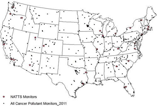
Air toxics data are based on 2003–2013 observations from monitoring sites across the United States. Ambient air toxics monitoring networks (Figure 1) include several hundred sites operated by states, local agencies, and tribes (SLTs) and 27 National Air Toxics Trends sites (NATTS). NATTS measure a core group of HAPs using established sampling and analysis protocols, whereas the SLT sites measure a variable number of HAPs at various frequencies using a variety of methodologies. In this paper we focus on 25 high-risk HAPs that include VOCs and semivolatile organic compounds (SVOCs) and metals. Sampling and analysis procedures conducted by SLTs followed EPA Compendium Methods (EPA, 1999a, 1999b). Noncarbonyl VOCs were collected by canisters and analyzed by gas chromatography/mass spectroscopy (GC/MS) or with continuous GCs and flame ionization detection (FID); carbonyls through dinitrophenylhydrazine (DNPH) coated cartridges followed by high-performance liquid chromatography (HPLC); polycyclic aromatic hydrocarbons (PAHs) through high-volume sampling with XAD resin and polyurethane foam (PUF) cartridges followed by GC/MS; and metals sampled through a variety of low- and high-volume filtration followed by x-ray diffraction (XRF) or inductively coupled plasma mass spectroscopy (ICPMS). Typically, sample collection periods were 24 hr and conducted every 6 days throughout each year. VOC data from the Photochemical Assessment Monitoring Stations (PAMS) that met completeness criteria, discussed later, either were sampled continuously through automated GC, reported hourly, by canisters at 3-hr intervals, or at 24-hr intervals.

Figure 1. 2011 Locations of hazardous air pollutant monitoring sites representing more than 200 sites operated by states, local agencies, and tribes have submitted data to EPA’s Air Quality System. With the exception of the NATTS, several sites in this map operate infrequently.

Data were obtained from Phase 9 of EPA’s Air Toxics Monitoring Archive for the years 1990–2013 (http://www.epa.gov/ttn/amtic/toxdat.html#data). Archive updates occur at between 1 and 2 years. Most of the data from the Phase 9 (latest update) archive (> 90%) are from the EPA’s Air Quality System (AQS), EPA’s database housing ambient observations. SLTs are required to submit data generated from EPA’s NATTS network and the Urban Air Toxics Monitoring Program (UATMP) to AQS, and are encouraged to submit other air toxics measurements to AQS. The UATMP provides centralized laboratory analytical support for air toxics networks.

Annual statistics were computed from daily averages for each site location from various networks with a mix of sampling periods and frequencies. Data completeness criteria required a minimum of 18 hr sampled over each 24-hr period and 75% completeness of daily values each quarter—that is, 6 days for 1-in-12 day sampling, 12 days for 1-in-6 day sampling, and 24 days for 1-in-3 day sampling, for a minimum of 3 quarters of the year. In cases with colocated measurements, data were averaged at the site level. Data below MDLs were included and the relative percentages of data below MDLs are reported.

Cancer and noncancer risks are calculated by relating annual concentrations (µg/m³) to EPA Unit Risk Estimates (URE) and Reference Concentrations (RfC) that represent the 1-in-a-million risk estimate associated with a concentration for each HAP (Table 1; EPA, 2014). While most cancer risk estimates are based on the upper confidence limit of the fitted dose-response curve, the values for some pollutants (e.g., benzene, chromium, nickel) are based on maximum likely estimation.

Table 1. Concentrations associated with risk for selected HAPs.

Pollutant	1 per 10^6 cancer risk (µg/m^3)	Hazard quotient = 1 (µg/m^3)
Chromium(VI)	8E-05	0.1
Arsenic	2E-04	0.015
Beryllium	4E-04	0.02
Cadmium	6E-04	0.01
Benzo[a]pyrene	6E-04	N/A
Ethylene dibromide	2E-03	9
Nickel	2E-03	0.09
Ethylene oxide	0.01	30
Acrylonitrile	0.01	2
Naphthalene	0.03	3
1,3-Butadiene	0.03	2
Ethylene dichloride	0.04	2400
Formaldehyde	0.08	9.8
1,4-Dichlorobenzene	0.09	800
Vinyl chloride	0.11	100
Benzene	0.13	30
Carbon tetrachloride	0.17	100
Trichloroethylene	0.21	2
Ethylbenzene	0.40	1000
Acetaldehyde	0.45	9
Tetrachloroethylene	3.8	40
Methylene chloride	62.5	600
Chloroform	N/A	98
Toluene	N/A	5000
Lead	N/A	0.15
Manganese	N/A	0.3
Acrolein	N/A	0.02

A linear dose-response relationship is assumed for all calculations. While the results reported here focus on 25 HAPs, all available HAPs observations meeting completeness criteria were used to calculate total risk by site location. Results are delineated by urban and rural site location and by network type (NATTS and SLTs) to examine representativeness of NATTS with respect to a denser network.

Trends from 2003–2013 were assessed using Spearman’s rank correlation (Myers and Well, 2003).

Results and discussion

Current year concentration and risk estimates based on NATTS

Observed HAPs for 2011 span a broad range of concentrations with high-volume VOCs (e.g., formaldehyde, acetaldehyde, benzene, toluene) typically 1 to 5 µg/m³ and halogenated organics, except for methylene chloride, and metals 2 and 3 orders magnitude lower, respectively (Figure 2 and Table 1). Concentrations are reported here in mass units (Table 2) consistent with health benchmark targets (Table 1), enabling screening estimates of exposure associated with risks that range from 30 to 190 per million with an average of 66 per million and all but seven sites exceeding 50 per million (Figures 3 and 4). Note that these estimates are representative of monitor locations and may not represent population risks. While risks were computed from as many as 41 HAPs measured at the sites, most of the risk is dominated by benzene, formaldehyde, naphthalene, 1,3-butadiene, acetaldehyde, nickel, arsenic, and carbon tetrachloride. Formaldehyde comprises most of the risk exceeding 10 per million at all sites. Risk estimates are dependent on the current Integrated Risk Information System (IRIS) formaldehyde value that is undergoing review (EPA, 1999a). Clearly, any substantive change would influence the relative contribution of risk associated with formaldehyde. In addition to formaldehyde, benzene and acetaldehyde risks exceed 1 per million at all sites;, and arsenic exceeds 1 per million at all but one site (La Grande, OR).

Table 2. 2011 concentration statistics by pollutant and NATTS location.

Note: Orange shading represents mean values above cancer risk benchmarks; yellow shading represents high percentage values less than MDL.

Table 3. 2011 annual HAPs concentrations at NATTS sites meeting MDL and risk thresholds.

	Percent sites with concentrations >			Percent sites with MDL > 1/10^6 risk benchmark^1
Species	MDL	1/10^6 cancer risk	10/10^6 cancer risk
Formaldehyde	100%	100%	100%	31%
Naphthalene (total tsp and vapor)	99%	85%	0%	0%
Acetaldehyde	99%	100%	0%	4%
Benzene	97%	100%	15%	7%
Arsenic Pm10 Lc	88%	96%	0%	15%
Carbon tetrachloride	87%	89%	0%	33%
Methylene chloride	83%	0%	0%	0%
Ethylbenzene	80%	32%	0%	4%
Chromium(VI) (LC)	75%	4%	0%	0%
Nickel Pm10 Lc	75%	19%	0%	4%
Benzo[b]fluoranthene	74%	0%	0%	0%
Cadmium Pm10 Lc	69%	7%	0%	4%
Benzo[e]pyrene(Tsp)	64%	0%	0%	0%
Benzo[g,h,i]perylene	49%	0%	0%	0%
1,3-Butadiene	48%	67%	0%	56%
Tetrachloroethylene	45%	0%	0%	0%
Benzo[k]fluoranthene	35%	0%	0%	0%
Ethylene dichloride	34%	30%	0%	61%
Benz[a]anthracene (total tsp and vapor)	33%	0%	0%	0%
Benzo[a]pyrene (total tsp and vapor)	33%	0%	0%	0%
p-Dichlorobenzene	19%	19%	0%	86%
Acrylonitrile	18%	36%	0%	100%
Perylene (total tsp and vapor)	7%	0%	0%	0%
Trichloroethylene	6%	0%	0%	30%
Vinyl chloride	2%	0%	0%	27%
trans-1,3-Dichloropropylene	1%	0%	0%	16%

Note: ¹MDLs are calculated frequently, often on a site basis, leading to variable MDLs.

Figure 2. 2011 HAPs annual average concentration distributions across NATTS and SLT sites (left) and just NATTS (right). Boxes show 10th (left whisker), 25th (left end of box), 50th, 75th (right end of box), and 90th (right whisker) percentile values of the site means. Solid dots show the mean across all sites. Box color is based on number of sites. Squares show the distribution of the MDLs: left is 10th percentile, X is 50th percentile, and the right side square reflects the 90th percentile of the MDL.

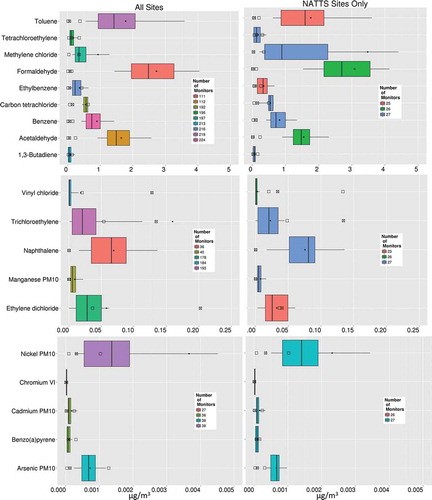
Figure 3. Cancer risk per million population by pollutant based on 2011 concentrations across National Air Toxics Trends Sites (NATTS). The right panel excludes formaldehyde to focus on HAPs more closely associated with anthropogenic emissions.

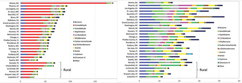
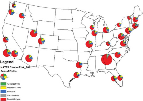
Figure 4. Spatial distribution of NATTS sites and risk contributions based on 2011 concentrations.

Major national and regional-scale patterns emerge for several relatively high-concentration gases. Elevated formaldehyde at the Atlanta, GA, site illustrates the regional- and urban-scale features of the highest national HAPs risk driver. Greater than 50% of formaldehyde in the southeastern United States. is attributable to biogenic emissions through a combination of direct formaldehyde releases and secondary formation (Luecken et al., 2012). Primary and secondarily formed contributions of formaldehyde from on-road vehicles combined with biogenic emissions lead to high concentrations in urban areas located in biogenically rich regions exemplified by Atlanta, GA.

Relative to other high-concentration gases, carbon tetrachloride concentrations (Figure 2) exhibit limited variation across sites, which is consistent with long atmospheric lifetimes (>20 years; Allen et al., 2009) and decreased use in industrial applications. Risks from carbon tetrachloride range from 3 to 4 per million across most sites. Benzene, toluene, ethylbenzene and 1,3-butadiene, and acetaldehyde are prevalent at all locations, indicative of on-road vehicle source contributions throughout the country. Benzene is the most ubiquitous and highest national risk driver of anthropogenic dominant HAPs (Figure 3).

Elevated nickel at the Bronx site (Figure 3), associated with residual fuel oil combustion (Peltier and Lippman, 2010), contrasts with the homogeneous levels of most HAPs across the NATTS and demonstrates the multiple spatial scale complexity of HAPs levels. From a national perspective, HAPs risk associated with regional and well-dispersed pollutants from natural and mobile sources contribute significantly to total risk across all populations, but the local-scale exposures to unique source types and pollutants may be elevated and a cause for concern (Jia and Foran, 2013). The observed higher values at the Bronx site have led New York to enact rules phasing out use of number 4 and number 6 fuel oil over the next two decades (Kheirbek et al., 2013).

Previous assessments have indicated that acrolein is the highest non-cancer-related risk HAP; however, it is not included in these analyses (Woodruff et al., 2007; deCrasto, 2014). There are substantial uncertainties in acrolein measurements due to postcollection reactions inside canisters and stability of calibration standards (EPA, 2010). Methodological improvements largely rely on best practices related to canister cleaning, speed of sample transfer and analysis, and optimizing stability and concentration of calibration standards. Diesel PM is not included in this measurement study as there is limited consensus regarding the representativeness of available surrogate measurements, such as elemental carbon through thermo-optical analysis.

Trends

Decreasing trends of the noncarbonyl VOCs (NCVOCs) with a strong mobile source signature (benzene, toluene, 1,3 butadiene and ethylbenzene) are observed at most NATTS (Figure 5), reflecting mobile source emission reductions. A series of vehicle and fuel regulations addressing onroad and nonroad emissions, such as the 2000 Tier II (CFR, 2000) and 2001–2007 MSAT rules (Code of Federal Regulations [CFR], 2001, 2007) are associated with NCVOC reductions. For example, MSAT imposes a reduction of benzene volume fraction in gasoline from about 1% in 2001 to 0.62 % in 2011. The aggregate contributions of fleet turnover, reformulated gasoline (RFG), and fuel standards explain reductions in species like benzene. NCVOC reductions also can be attributed to improved practices and controls in petrochemical processing and various chemical manufacturing industries, particularly in Houston, TX, and similar areas with significant petrochemical/chemical industry footprints. Although benzene concentration reductions across NATTS average 4.8% per year over the 14-year period (Figure 6), a noticeable leveling since 2003–2004 is evident in cities such as Washington, DC, and Chicago, IL (Figure 7), in contrast to previous significant reductions up to 2003. Other cities, such as Roxbury, MA (Figure 8), demonstrate strong benzene declines through 2010. These city-specific responses illustrate variations likely associated with regional differences in fuel supply and vehicle mixes, source composition, and economic trends.

Figure 5. Spearman coefficients indicating significance of upward and downward trends based on NATTS data from 2003–2014. Green, decrease; red, increase; yellow, insignificant.

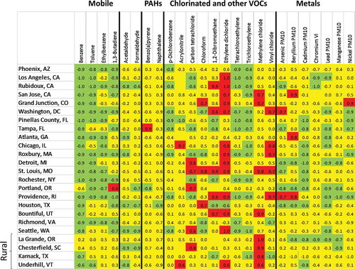
Figure 6. 2003–2012 Benzene trends at NATTS and SLTs.

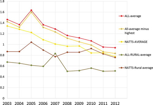
Figure 7. 2000–2013 Benzene trends at NATTS in Chicago (top) and Washington, DC. Box shows 10th (whisker), 25th (bottom of box), 50th, 75th (top of box), and 90th (whisker) percentile values of the site means. Color of box is based on number of sites. Solid dots show the site mean. Hollow circles show the mean MDL. Red solid line identifies the inhalation exposure concentration associated with a 1 per million cancer risk. The symbol key includes symbols to indicate MDL values beyond axis range and hazard quotient value for non-cancer-based risk, neither of which is applicable for these benzene results.

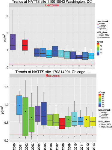
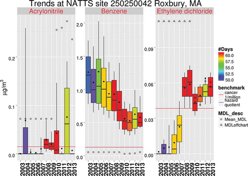
Figure 8. Trends of three HAPs at Roxbury, MA, illustrating differences in MDL and cancer risk threshold values. Box shows 10th (whisker), 25th (bottom of box), 50th, 75th (top of box), and 90th (whisker) percentile values of the site means. Color of box is based on number of sites. Solid dots show the site mean. Hollow circles show the mean MDL. Hollow triangle indicates that the mean MDL is larger than the upper range of the chart. Red solid line shows the inhalation exposure concentration associated with a 1 per million cancer risk.

Two chlorinated organic HAPs, trichloroethylene and tetrachloroethylene, also exhibit declining concentrations at several urban sites. Both are solvents that have been used in metals degreasing and in the case of tetrachloroethylene in dry cleaning. Tetrachloroethylene concentrations track the phase-out of tetrachloroethylene use in dry-cleaning operations throughout the last decade brought about by the 2008 NESHAP (CFR, 2008). Rising concentration trends for ethylene dichloride and methylene chloride are unique compared to other HAPs analyzed at the NATTS (Figure 5); these increases do not track the air emissions trends in EPA’s toxics release inventory (EPA, 2013). Lead and cadmium also exhibit decreasing concentration trends, consistent with the EPA’s Toxics Release Inventory (TRI) indicating decadal emissions reductions of 80% and 94% for lead and cadmium, respectively.

With the exception of methylene chloride, HAPs at rural sites, with a qualitative definition based on relative distance from major sources and roadways, do not show consistent trends (Figure 5). While delineating signal changes in low concentration rural environments is challenging, the results from NCVOCs are surprising, as impacts of fuel and motor vehicle changes should be consistent in urban and rural or regional settings.

Minimum detection limit (MDL) and risk benchmarks

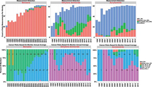
Characterizing 187 HAPs that span a broad range of ambient levels and instrument capabilities is challenging. Many HAPs have a significant percentage of data reported below minimum detection limit (MDL), which limits our ability to assess trends or evaluate models. To illustrate uncertainties based on the frequency of observations that exceed MDLs and the relationship of risk benchmarks to MDLs and reported concentrations, we highlight benzene, ethylene dichloride, and acrylonitrile. Because observed benzene concentrations are consistently above MDLs, and benzene MDLs are mostly below the cancer risk benchmark representative of 1 in 1 million risk (Figure 9), we are more confident in the interpretation of these concentration and risk values and their general downward trends. For ethylene dichloride and acrylonitrile, concentrations typically are below the MDLs and near the 1 in 1 million risk benchmarks (Figure 9), which reduce confidence in data interpretation. Greater than 70% of all ethylene dichloride and acrylonitrile observations exhibit concentrations associated with less than 1 in 1 million risk, and nearly 90% of observations are below MDL or record a nondetect. Table 3 lists common HAPs with respect to the frequency of observations that exceed MDLs and 1 in 1 million cancer risk concentration benchmarks, providing a cursory view of the relative confidence of HAPs measurements in characterizing uncertainties in a risk context. It also indicates that more than 20% of HAPs MDLs exceed 1 in 1 million at more than half the sites. The acrylonitrile MDL exceeds 1 in 1 million at all sites. The pollutants with MDLs above the 1 in 1 million risk benchmark also are largely measured below MDL.

Figure 9. Distribution of benzene, ethylene dioxide, and acrylonitrile observations above MDLs and risk thresholds for all NATTS.

Approaches for the use of data below MDLs in air toxics data analyses include discarding data, using all data, or applying a surrogate such as half the MDL value for data below MDLs. McCartney et al. (2007, 2009) reasoned that applying MDL/2 provided annual average results are statistically insignificant with more complex statistical filtering procedures, thus rationalizing the use of a simple surrogate. In this study, we chose to use all data meeting completeness criteria complemented by analyses exhibiting fraction of data exceeding MDLs. Nondetects were treated as zero values.

Air monitoring network considerations

Previous reviews of national monitoring networks (Dmerjian, 2000; Scheffe et al., 2012) have noted the challenges faced by the air toxics monitoring infrastructure. The variety of HAPs covering VOCs, SVOCs, and metals with a range of atmospheric lifetimes that act across multiple spatial scales, important to HAP policy, challenges classic monitoring network design relying on fixed-site, labor-intensive operations. Depending on the particular HAP, air toxics can be viewed as having a dominant local, urban, regional, or global scale influence. The evidence suggests that the basic concentration patterns and trends generated by NATTS are consistent with the larger air toxics data base (Figure 2), thus raising the confidence that NATTS adequately captures general concentration profiles in major urban centers. Clearly, routine national monitoring networks, such as the NATTS, are not capable of delineating the fine-scale spatial texture often associated with a complex mix of sources and extremely variable local-scale meteorology, where even well-dispersed HAPs such as benzene and formaldehyde exhibit significant gradients at subkilometer scales (Whitworth et al., 2011, Kheirbek et al., 2012). Moreover, a lack of air toxics regulatory drivers comparable to those for NAAQS monitoring combined with labor-intensive sampling and analysis protocols suggests that traditional network expansion may not be feasible. Consequently, any growth in our air toxics monitoring programs must rely on leveraging available and emerging technologies to integrate into the existing monitoring infrastructure. The emphasis on chronic long-term exposures associated with cancer risk and reliance on annual concentration averages minimize the need for highly time-resolved measurements and consequent resource demands. However, availability of more highly time-resolved data would support risk assessments evaluating acute risks and model evaluation efforts.

As currently configured, the NATTS and SLT networks are best suited for capturing urban-scale (5–50 km) conditions with the SLT sites offering flexibility for agencies to focus on specific HAPs or source mixtures of interest. The recent growth of small sensor technology applications has focused on criteria air pollutants such as ozone and nitrogen dioxide (Snyder et al., 2013). Pending further development, these technologies may be well suited to address many of the unique localized aspects of air toxics exposures, perhaps offering a fine spatial scale complement to the existing networks. In the near term, passive samplers may provide a low-cost option for measuring several HAPs (Mason et al., 2011). High resource levels required to deploy more advanced technologies such as lidars and mass spectrometry typically have been limited to special studies or specific source characterization and not integrated into our networks (Weibring et al., 2003; Knighton et al., 2012). Emerging techniques such as submillimeter wave spectroscopy (Medvedev et al., 2010), quantum cascade laser (QCL, Elia et al., 2009), and MultiAXis differential optical absorption spectroscopy (MAXDOAS; Pinardi et al., 2013) are being explored by EPA to improve carbonyl HAP measurements.

Coinciding with the NATTS deployment, EPA issued a series of community air monitoring grants starting in 2003 intended to complement the NATTS by providing flexibility to address the unique issues facing SLT organizations across the nation (Sonoma Technology, Inc. [STI], 2013). Future grants potentially can complement other observation programs. In addition to these community air toxics monitoring grants, SLTs have some discretion within available albeit very limited resources to tailor observation programs to address discrete, near-source, localized exposures.

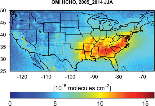
Remote sensing of formaldehyde provides an underused and potentially valuable source of regional scale observations. Over the last decade, European and U.S.-based instruments on polar orbiting satellites have yielded images of formaldehyde patterns (Figure 10) consistent with the spatial texture provided by land based observations (Figure 4). Several studies have demonstrated strong associations between satellite sensors and lower tropospheric formaldehyde observations from ground-based and aircraft platforms, generally with a focus on characterizing isoprene emissions for global-scale air quality modeling applications (Boeke et al., 2011; Chance et al., 2000; Duncan et al., 2009; Jones et al., 2009; Millet et al., 2006; Millet et al., 2008). From a network perspective, satellite-based data arguably provide a useful regional signal on formaldehyde distribution in the lower troposphere. Boeke et al. (2011) demonstrated the ability of the Ozone Monitoring Instrument (OMI) on board the AURA satellite of the Earth Observing System (EOS) to also delineate urban- and regional-scale signals. Satellite-based ratios of glyoxal to formaldehyde potentially can be used to assess the relative source contributions associated with natural and anthropogenic emissions (DiGangi et al., 2012). These applications of space-based formaldehyde observations rely on polar orbiting satellites typically generating two signals a day. Oversampling techniques in Houston, TX, suggest that satellite formaldehyde data also can delineate urban and regional air quality scale features (Zhu et al., 2014), implying far greater returns from the scheduled launching of Tropospheric Emissions: Monitoring of Pollution (TEMPO) by NASA in 2017, which will provide a near continuous supply of space-based observations, including formaldehyde.

Figure 10. Formaldehyde total column density sampled June–August of 2005–2014 based on OMI satellite data illustrating spatial pattern similar to land based observations. (Courtesy, Lei Zhu and Daniel Jacob, Harvard University/NASA Air Quality Applied Science Team.)

Conclusions

Characterizing ambient air toxics patterns across multiple spatial scales in the United States is a challenging task using data from our national monitoring networks. With the exception of carbon tetrachloride, most of these higher risk HAPs are derived from combustion related sources (transportation, residential and commercial heating, energy generation, or industrial processing). Formaldehyde, the highest national HAP risk driver, is unique, given the significant contributions from natural and anthropogenic sources and secondary atmospheric formation. These broad source attribution descriptions reflect a limit of the NATTS that are constrained to 27 locations nationally and were designed to provide a broad characterization across the United States. Fixed site monitoring networks for air toxics provide limited capability to address local and broad regional scale air quality. Consequently, leveraging programs such as NASA’s forthcoming GEOstationary Coastal and Air Pollution Events (GEO-CAPE) mission and community based grants and new sensor technologies are necessary components of a future air toxics monitoring infrastructure.

It is not surprising that many HAPs exhibit declining concentration trends analogous to improvements in concentrations of criteria pollutant species and precursors (EPA, 2015b), given the commonality of source types, particularly combustion-based processes, shared by HAPs and criteria pollutants. A clear trend in formaldehyde is compromised by near constant and substantial emissions from natural sources.

The variety in MDLs and risk thresholds associated with 187 HAPs of concern clearly challenges the ability of existing technologies to characterize risk, particularly at low concentration levels and low-threshold risk HAPs. These concerns are less relevant for high-volume HAPs such as benzene and formaldehyde, which constitute a significant fraction of cancer risk nationally.

Given the paucity of monitoring sites and the need to account for 187 HAPs, we rely on air quality modeling to drive EPA’s NATAs. Observations from the nation’s land-based monitoring networks complement model-based risk assessments by providing a means of more frequently evaluating trends with a consistent information base for tracking exposure and attempting to infer progress from national rules that are reducing HAP emissions.

Looking ahead, the nation’s air toxics monitoring programs would benefit from a comprehensive assessment addressing objectives, design, and technology. Should model evaluation be a primary monitoring objective, given the reliance on air quality modeling for risk assessments? Should the NATTS continue as currently deployed, expanded or decreased in scope, or modified to better complement other observation programs? While suggestions have been raised here regarding leveraging other measurement efforts, a reasoned and coordinated strategy is called for to extract the most value in the current and foreseeable resource-constrained environment. One option is to adopt the recommendations on leveraging observation systems provided in the Air Quality Observations report produced by Committee on Environment, Natural Resources and Sustainability (CENRS, 2013). Those recommendation call for bridging multiple spatial scales, pollutants, and environmental media through an organized multiple-stakeholder partnership that collectively adopts a measurement mission broader in scope than a single organization-based focus.

Acknowledgments

The authors appreciate the efforts of all anonymous reviewers to review this paper and provide suggestions, as well as those of Richard Cook, James Hemby, Mark Houyoux, Mike Koerber, and Ted Palma of the EPA. We also appreciate publications support from the Coordinating Research Council.

Additional information

Notes on contributors

Richard Scheffe

Madeleine Strum and Richard Scheffe are engineers in the Air Quality Assessment Division of EPA’s Office of Air Quality Planning and Standards in Durham, NC.

References

- Allen, N.D.C., P.F. Bernath, C.D. Boone, M.P. Chipperfield, D. Fu, G.L. Manney, D.E. Oram, G.C. Toon, and D.K. Weisenstein. 2009. Global carbon tetrachloride distributions obtained from the Atmospheric Chemistry Experiment (ACE). Atmos. Chem. Phys. 9:7449–59. doi:10.5194/acp-9-7449-2009
- Boeke, N.L., J.D. Marshall, S. Alvarez, K.V. Chance, A. Fried, T.P. Kurosu, B. Rappenglück, D. Richter, J. Walega, P. Weibring, and D.B. Millet. 2011. Formaldehyde columns from the Ozone Monitoring Instrument: Urban versus background levels and evaluation using aircraft data and a global model. J. Geophys. Res. 116:D05303. doi:10.1029/2010JD014870
- Bortnick, S.M., and S.L. Stetzer. 2002. Sources of variability in ambient air toxics monitoring data. Atmos. Environ. 36:1783–91. doi:10.1016/S1352-2310(02)00160-7
- Chance, K., P.I. Palmer, R.J.D. Spurr, R.V. Martin, T.P. Kurosu, and D.J. Jacob. 2000. Satellite observations of formaldehyde over North America from GOME. Geophys. Res. Lett. 27(21):3461–64. doi:10.1029/2000GL011857
- CENRS. 2013. Air Quality Observation Systems in the United States. Air Quality Research Subcommittee of the Committee on Environment, Natural Resources and Sustainability of the National Science and Technology Council. https://www.whitehouse.gov/sites/default/files/microsites/ostp/NSTC/air_quality_obs_2013.pdf
- Demerjian, K.L. 2000. A review of national monitoring networks in North America. Atmos. Environ. 34:1861–84. doi:10.1016/S1352-2310(99)00452-5
- George, B.J., B.D. Schultz, T. Palma, A.F. Vette, D.A. Whitaker and R.W. Williams. 2011. An evaluation of EPA’s National-Scale Air Toxics Assessment (NATA): Comparison with benzene measurements in Detroit, Michigan. Atmos. Environ. 45(19):3301–8. doi:10.1016/j.atmosenv.2011.03.031
- deCastro, B.R. 2014. Acrolein and asthma attack prevalence in a representative sample of the United States adult population 2000–2009. PLoS ONE 9(5). doi:10.1371/journal.pone.0096926
- DiGangi, J.P., S. B. Henry, A. Kammrath, E.S. Boyle, L. Kaser, R. Schnitzhofer, M. Graus, A. Turnipseed, J.-H. Park, R. J. Weber, R.S. Hornbrook, C.A. Cantrell, R.L. Maudlin III, S. Kim, Y. Nakashima, G.M.Wolfe, Y. Kajii, E.C. Apel, A.H. Goldstein, A. Guenther, T. Karl, A. Hansel, and F.N. Keutsch. 2012. Observations of glyoxal and formaldehyde as metrics for the anthropogenic impact on rural photochemistry. Atmos. Chem. Phys. 12:9529–43.www.atmos-chem-phys.net/12/9529/2012/ doi:10.5194/acpd-12-6049-2012
- Duncan, B.N., Y. Yoshida, M. R. Damon, A.R. Douglass, and J.C. Witte. 2009. Temperature dependence of factors controlling isoprene emissions. Geophys. Res. Lett. 36:L05813, doi:10.1029/2008GL037090
- Elia, A., C. Di Franco, V. Spagnolo, P.M. Lugarà, and G. Scamarcio. 2009. Quantum cascade laser-based photoacoustic sensor for trace detection of formaldehyde gas. Sensors 9:2697–705. doi:10.3390/s90402697
- ICF International. 2011. An Overview of Methods for EPA’s National-Scale Air Toxics Assessment, prepared for U.S. EPA Office of Air Quality Planning and Standards. Durham, NC: ICF International. http://www.epa.gov/ttn/atw/nata2005/index.html.
- Jia, C., and J. Foran. 2013. Air toxics concentrations, source identification, and health risks: An air pollution hot spot in southwest Memphis, TN. Atmos. Environ. 81:112–16. doi:10.1016/j.atmosenv.2013.09.006
- Jones, N.B., K. Riedel, W. Allan, S. Wood, P. I. Palmer, K. Chance, and J. Notholt. 2009. Long-term tropospheric formaldehyde concentrations deduced from ground-based Fourier transform solar infrared measurements. Atmos. Chem. Phys. 9:7131–42. doi:10.5194/acp-9-7131-2009
- Kimbrough, S., T. Palma, and R. Baldauf. 2014. Analysis of mobile source air toxics (MSATs)-Near-road VOC and carbonyl concentrations. J. Air Waste Manage. Assoc. 64(3):349–59. doi:10.1080/10962247.2013.863814
- Luecken, D.J., W.T. Kutzell, M.L. Strum, and G.A. Pouliot. 2012. Regional sources of atmospheric formaldehyde and acetaldehyde, and implications for atmospheric modeling. Atmos. Environ. 47:477–90. doi:10.1016/j.atmosenv.2011.10.005
- Kheirbek, I., S. Johnson, K. Ito, T. Matte and D. Kass, S.A. Caputo, S. Mahnovski, C.H. Strickl and, A. Licata, H. Eisl, J. Gorczynski, S. Markowitz, and Z. Ross. 2012. New York City Trends in Air Pollution and its Health Consequences. http://www.nyc.gov/html/doh/downloads/pdf/environmental/air-quality-report-2013.pdf.
- Kheirbek, I., S. Johnson, Z. Ross, G. Pezeshki, K. Ito, H. Eisl, and T. Matte. 2013. Spatial variability in levels of benzene, formaldehyde, and total benzene, toluene, ethylbenzene and xylenes in New York City: a land-use regression study. Environ. Health 11:51. doi:10.1186/1476-069X-11-51
- McCarthy, M. C., H.R. Hafner, and S. Montzka. 2006. Background concentrations of 18 air toxics for North America. J. Air Waste Manage. Assoc. 56(1):7180–7194. doi:10.1080/10473289.2006.10464436
- McCarthy, MC., H.R. Hafner, L.R. Chinkin, and J.G. Charrier. 2007. Temporal variability of selected air toxics in the United States, Atmos. Environ. 41:7180–94. doi:10.1016/j.atmosenv.2007.05.037
- McCarthy, M. C., T.E. O’Brien, J.G. Charrier and H.R. Hafner. 2009. Characterization of the chronic risk and hazard of hazardous air pollutants in the United States using ambient monitoring data. Environ. Health Perspect. 117(5):790–96. doi:10.1289/ehp.11861
- Millet, D.B., D.J. Jacob, S. Turquety, R.C. Hudman, S. Wu, A. Fried, J. Walega, B.G. Heikes, D.R. Blake, H.B. Singh, B.E. Anderson, and A.D. Clarke. 2006. Formaldehyde distribution over North America: Implications for satellite retrievals of formaldehyde columns and isoprene emission. J. Geophys. Res. 111:D24S02, doi:10.1029/2005JD006853, 2006
- Millet, D.B., D.J. Jacob, K.F. Boersma, T.-M. Fu, T.P. Kurosu, K. Chance, C.L. Heald, and A. Guenther. 2008. Spatial distribution of isoprene emissions from North America derived from formaldehyde column measurements by the OMI satellite sensor. J. Geophys. Res. D02307. doi:10.1029/2007JD008950
- Myers, J.L., and A.D. Well. 2003. Research Design and Statistical Analysis, 2nd ed. Lawrence Erlbaum Associates.
- Peltier, R.D., and M. Lippmann. 2010. Residual oil combustion: 2. Distributions of airborne nickel and vanadium within New York City. J. Expos. Sci. Environ. Epidemiol. 20:342–50. doi:10.1038/jes.2009.28
- Pinardi, G., M. Van Roozendael, N. Abuhassan, C. Adams, A. Cede, K. Cl´emer, C. Fayt, U. Frieß, M. Gil, J. Herman, C. Hermans, F. Hendrick, H. Irie, A. Merlaud, M. Navarro Comas, E. Peters, A.J.M. Piters, O. Puentedura, A. Richter, A. Schönhardt, R. Shaiganfar, E. Spinei, K. Strong, H. Takashima, M. Vrekoussis, T. Wagner, F. Wittrock, and S. Yilmaz. 2013. MAX-DOAS formaldehyde slant column measurements during CINDI: Intercomparison and analysis improvement. Atmos. Meas. Technol. 6:67–185. doi:10.5194/amt-6-167-2013
- Scheffe, R.D., J.R. Brook, and K.L. Demerjian. 2012. Air quality measurements. In Technical Challenges of Multipollutant Air Quality Management, 339–393, ed. G.M. Hidy, J.R. Brook, K.L. Demerjian, L.T. Molina, W.T. Pennell, R.D. Scheffe. New York, NY: Springer.
- Snyder, E.G., T.H. Watkins, P.A. Solomon, E.D. Thoma, R.W. Williams, G.S.W. Hagler, D. Shelow, D.A. Hindin, V.J. Kilaru, and P.W. Preuss. 2013. The changing paradigm of air pollution monitoring. Environ. Sci. Technol. 47:11369−77. doi:10.1021/es4022602
- Sonoma Technology, Inc. 2013. A Synthesis of Completed Community Scale Air Toxics Monitoring Projects. Petaluma, CA: Sonoma Technology, Inc. STI-910313-5469-FR.
- U.S. Environmental Protection Agency. 1999a. Integrated Risk Information System (IRIS) on Formaldehyde. Washington, DC: National Center for Environmental Assessment, Office of Research and Development.
- U.S. Environmental Protection Agency. 1999b. Compendium of Methods for the Determination of Toxic Organic Compounds in Ambient Air, 2nd ed. EPA/625/R-96/010b. http://www.epa.gov/ttn/amtic/files/ambient/airtox/to-15r.pdf
- U.S. Environmental Protection Agency. 2007. Control of Hazardous Substances from Mobile Sources. 40 CFR 7 (37).
- U.S. Environmental Protection Agency. 2010. Data Quality Evaluation Guidelines for Ambient Air Acrolein Measurements. http://www.epa.gov/ttnamti1/files/ambient/airtox/20101217acroleindataqualityeval.pdf.
- U.S. Environmental Protection Agency. 2013. Toxics Release Inventory National Analysis. http://www2.epa.gov/toxics-elease-inventory-tri-program/2013-toxics-release-inventory-national-analysis.
- U.S. Environmental Protection Agency. 2014. Dose-Response Assessment for Assessing Health Risks Associated With Exposure to Hazardous Air Pollutants. http://www2.epa.gov/fera/dose-response-assessment-assessing-health-risks-associated-exposure-hazardous-air-pollutants.
- U.S. Environmental Protection Agency. 2015a. National Emission Standards for Hazardous Air Pollutants. 40 CFR, Part 61. http://www.epa.gov/ttn/atw/mactfnlalph.html.
- U.S. Environmental Protection Agency. 2015b. Air Quality Trends. http://www.epa.gov/airtrends/aqtrends.html.
- Whitworth, K.W., E. Symanski, D. Lai, and A.L. Coker. 2011. Kriged and modeled ambient air levels of benzene in an urban environment: an exposure assessment study. Environ. Health 10:21. doi:10.1186/1476-069X-10-21
- Woodruff, T.J., E.M. Wells, D.E. Burgin, and D.A. Axelrad. 2007. Estimating risk from ambient concentrations of acrolein across the United States. Environ. Health Perspect. 115(3):410–15. doi:10.1289/ehp.9467
- Zhu, L., D.J. Jacob, L.J. Mickley, E.A. Marais, D.S. Cohan, Y. Yoshida, B.N. Duncan, G.G. Abad, and K.V. Chance. 2014. Anthropogenic emissions of highly reactive volatile organic compounds in eastern Texas inferred from oversampling of satellite (OMI) measurements of HCHO columns. Environ. Res. Lett. 9:114004. doi:10.1088/1748-9326/9/11/114004