ABSTRACT
Although networks of environmental monitors are constantly improving through advances in technology and management, instances of missing data still occur. Many methods of imputing values for missing data are available, but they are often difficult to use or produce unsatisfactory results. I-Bot (short for “Imputation Robot”) is a context-intensive approach to the imputation of missing data in data sets from networks of environmental monitors. I-Bot is easy to use and routinely produces imputed values that are highly reliable. I-Bot is described and demonstrated using more than 10 years of California data for daily maximum 8-hr ozone, 24-hr PM2.5 (particulate matter with an aerodynamic diameter <2.5 μm), mid-day average surface temperature, and mid-day average wind speed. I-Bot performance is evaluated by imputing values for observed data as if they were missing, and then comparing the imputed values with the observed values. In many cases, I-Bot is able to impute values for long periods with missing data, such as a week, a month, a year, or even longer. Qualitative visual methods and standard quantitative metrics demonstrate the effectiveness of the I-Bot methodology.Implications: Many resources are expended every year to analyze and interpret data sets from networks of environmental monitors. A large fraction of those resources is used to cope with difficulties due to the presence of missing data. The I-Bot method of imputing values for such missing data may help convert incomplete data sets into virtually complete data sets that facilitate the analysis and reliable interpretation of vital environmental data.
Introduction
Networks of environmental monitors provide data needed for critical decisions that affect public and environmental health. Air quality monitors provide data needed to advance the science of air pollution and to inform efforts to manage air pollution with respect to health risks, and meteorological monitors provide data needed for many purposes, including the characterization of atmospheric conditions that affect levels of air pollution.
Even the best networks of environmental monitors do not operate flawlessly, and instances of missing values can obscure the meaning that the networks intend to reveal. Various ways of coping with the effects of missing data have been developed, ranging from simplistic (do nothing) to complex (an ad hoc approach for each situation). A desirable alternative is to impute reliable values for the missing data. If reliable imputed values are combined with measured data, the completed data sets may enable analyses that are more convenient and more convincing. They may be more convenient, because steps to cope with missing values need not be taken. They may be more convincing, when uncertainties concerning the effects of missing data are largely removed.
A system for imputing values for missing data has been developed at the California Air Resources Board (CARB). The system takes advantage of natural connections within data sets collected from networks of environmental monitors. The method is context intensive, as it searches for the best available connections site by site, day by day, even hour by hour in constantly changing seasonal and diurnal windows. Within each context-intensive setting, the calculation is currently done by simple regression (a single “x” variable to predict a missing value of the “y” variable). The method is called “I-Bot” (short for Imputation Robot), because it uses simple procedures and minimal assumptions as it imputes one value within the specific context-intensive setting for each particular missing value.
Imputed values are estimates of what would have been measured if the monitoring system had operated as intended. The data that are available provide the context for determining imputed values. An imputed value represents what should be expected within a particular context and is determined by relationships that occur in the measured data within that context. When data are highly structured, with a limited number of repeating patterns, imputing values for missing data can be straightforward. However, imputing values for missing environmental data is complicated by the fact that the environmental context is constantly changing, and patterns may change quickly, unpredictably, or both.
Imputing values for missing environmental data has been studied using a wide variety of approaches. Schneider applied a regularized EM (estimate, maximize) algorithm (ridge regression being the regularized component) to impute values for missing climate data (Schneider, Citation2001). Junninen et al. considered several imputation methods applied to both air pollution and meteorological variables (Junninen et al., Citation2004). Plaia et al. proposed an imputation method based on additive effects and used data for particulate matter to compare its performance with several alternative imputation methods (Plaia et al., Citation2006). Le et al. tested a number of ways to impute missing values in air toxics data for 70 volatile organic compounds (Le et al., Citation2007).
Perhaps the most common way of addressing the issue of missing values in environmental data sets is to establish criteria for deciding when data sets are complete enough to be used; thereafter, the effects of any missing values are ignored. Many federal and state regulations that rely on environmental data include completeness criteria that the data must satisfy. Although regulations rarely allow values to be imputed explicitly, certain characteristics of the missing data are, in fact, imputed implicitly. Consider, for example, an incomplete data set that satisfies the criteria for completeness and that also satisfies a regulatory standard; this situation implies that the outcome would not have changed if a truly complete data set had been available. So, the missing values are implicitly imputed to be such that the regulatory decision would not change.
When the decision is made to impute values for missing data, the literature on the topic may or may not be helpful. For example, a simple interpolation method may work well for short gaps in data series that are relatively smooth in time or space or both. Unfortunately, many environmental variables are not smooth in time or space, and sudden, unusual changes may occur. Imputation methods for multihour or multiday gaps may also be available, but many environmental data sets are subject to much larger gaps in time (a month or more) and in space (20 km or more) and may include variable and atypical patterns.
Fortunately, when networks of environmental monitors are dense enough, the data sets they deliver typically contain strong internal connections that can be used in a single unified approach to address almost all instances of missing data. In California, air pollutants, such as ozone and fine particulate matter (aerodynamic diameter <2.5 μm; PM2.5), and meteorological parameters, such as temperature and wind speed, are measured by networks of hundreds of monitors containing strong internal connections. I-Bot was developed to find the best available relationships and use them to impute values for missing data.
Methods
When data from two sites are strongly related, their relationship can be used to impute missing values at one of the sites based on corresponding measured values at the other site. In quality assurance applications, sites whose data are strongly related are sometimes called “Buddy Sites” (U.S. Environmental Protection Agency [EPA], Citation2012; California Air Resources Board, Citation2006). In this paper, a monitor for which a value is missing is called the “Target Site” and a site used to impute the missing value is called the “Buddy Site.”
I-Bot methodology can be summed up in three steps that repeat for each and every missing value. First, select data for the current context (season, time of day, etc.) for the Target Site and for potential Buddy Sites. Second, evaluate the linear relationships between the observed data from the Target Site and the observed data from each potential Buddy Site. And third, use the observed value and the linear relationship for the most highly correlated Buddy Site to impute the missing value at the Target Site.
Rationale
Data from nearby sites are naturally related
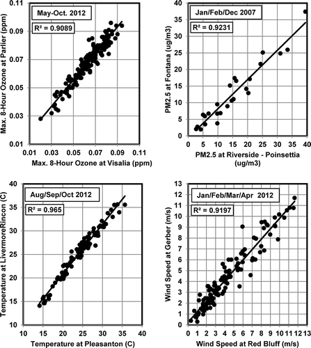
I-Bot methodology is motivated by a fundamental observation: data from networks of environmental monitors include naturally related, strongly correlated, subsets of monitors that share a common context. Atmospheric measurements tend to share a common context when the monitors are close to one another. Temperature, pressure, and humidity are often (though not always) strongly correlated over tens of kilometers, increasing and decreasing together from one hour to the next or one day to the next. Levels of air pollutants at nearby monitors are often strongly correlated for at least three reasons. First, the monitors may operate under (largely) shared atmospheric conditions that affect the dispersion and/or the emissions of pollutants. Second, patterns of human activities that produce pollutants in the general area are often highly repetitive by season of the year and time of day. And third, nearby monitors are frequently downwind of the same types of pollution sources for general categories of wind direction. provides examples of strong natural connections between pairs of sites in California.
Natural connections are dynamic
From hour to hour, day to day, season to season, or year to year, the best choice of Buddy Site for a given Target Site may change. Common reasons for a change in the best Buddy Site include the following: (1) the usual best Buddy Site is also missing data; (2) prevailing wind patterns have changed with season or time of day, causing another site to be more correlated; and (3) a newly established site becomes the best Buddy Site because its data prove to be most highly correlated with the data from the Target Site. I-Bot naturally handles all these situations, and more, as it simply allows the data available for the current context to direct the “best” choice of Buddy Site for each instance of missing data.
The best connections may be obscured when the context is too wide
The best connections between the data sets for different monitors typically occur in highly restricted contexts. If a wide context is selected, the connection between the Target and Buddy Sites may look reasonably good, but better connections within narrower contexts may be missed. For example, linear relationships between sites are known to change from season to season and throughout the day. If the context for imputation today is taken to include the whole year and all hours of the day, the fidelity of the imputed values is likely to be adversely affected. Limiting the context to some weeks before and after the current date and to some hours before and after the current hour usually leads to imputed values with greater fidelity.
Prior knowledge of specific situations is not needed to justify or to apply the I-Bot approach. The general understanding that relationships between sites may be dynamic, not constant, is enough to start the imputation process with tight contexts and demanding criteria for success.
I-Bot addresses the entire data set in several iterations or “passes.” By gradually widening the defined context (more years involved) and/or relaxing the required criteria for success (lowering the required correlation) on successive passes, almost all missing values may eventually be satisfactorily imputed.
High-quality imputed values may later serve “as if” they were measured
High-quality imputed values created during earlier passes may serve during later passes “as if” they were measured values. This practice is especially helpful when imputing values for a large gap (multiple months or years) in a data set, as strong connections between Buddy Sites within a tight context in an earlier pass are allowed to express themselves in a later pass for which a wider context covers the large gap.
Performance can be evaluated empirically
Imputing values for measured data as if they were missing allows the I-Bot method to be evaluated empirically. The precision of each imputed value is estimated by the statistical model that determines the imputed value, but comparing imputed and measured values for groups of days or hours allows powerful post hoc evaluations of the imputation methodology. For example, performance when imputing values for large gaps can be tested by treating data for an entire year as if it is missing and then comparing the imputed values to the actual measured values. With the I-Bot system, this type of analysis is easily conducted.
Implementation
Implementation of the I-Bot approach is discussed in this section from an algorithmic design point of view, not a software-specific point of view. Imputed values used in this paper were produced with programs written by the primary author in Delphi (object pascal) as “console applications” that run in CommandPrompt windows (Win95 or higher). Although significant attention was given to the optimization of speed on a desktop personal computer, the content of this section is sufficient for others to prepare their own I-Bot systems using widely available programming resources for querying databases and for processing the resulting data sets.
The data for illustrations in this implementation section come from an imputation exercise for daily maximum 8-hr ozone at 295 monitoring sites in California from 1996 through 2012 (6210 days). The data set included 1.8 million placeholders, as all combinations of 295 sites and 6210 days were considered. For some of the placeholders, measured data were available, but for other placeholders, data were missing. For each placeholder, the I-Bot exercise attempted to determine an imputed value, whether or not a measured value was present.
Specification of the current context
The context for determining a daily imputed value includes distance, year(s), and season-within-year(s). For determining an hourly imputed value, the context also includes time-within-day. These context elements are addressed in turn.
Distance. A maximum distance from the Target monitor is selected, which was 100 km for the referenced ozone study. The max-distance parameter primarily affects the number of potential Buddy Sites that will be evaluated. For example, our current I-Bot system will consider up to 10 potential Buddy Sites, but for the ozone monitor at Blythe, California, only two Buddy Sites existed within the 100-km limit. Limiting the acceptable distance increases efficiency by avoiding needless evaluation of far-distant sites as potential Buddy Sites.
In some cases, a Target Site may have no adequate Buddy Site. An example in California is Echo Summit, an elevated site (~2250 m). Although this site’s nearest neighbors are less than 10 km distant around Lake Tahoe, they are 340 m lower in elevation and are not effective Buddy Sites for Echo Summit. In a recent imputation exercise, only 15% of days from May through October for the years 2011–2013 met the minimum correlation criterion required to proceed with an imputation at Echo Summit.
Year(s). Relationships between Target and Buddy Sites change from year to year for various reasons, such as significant changes in nearby emission sources. Therefore, a window of plus-and-minus “Y” years around the current date is set for I-Bot to use. For early passes through the data, Y is usually kept small (0 or 1). If Y is zero, only the current season window of ±D days is used. If Y is 1, then two more season windows are used, one centered on the current date minus 365 days and one centered on the current date plus 365 days. The season is kept the same within each of the years used in the imputation process.
In later “passes” through the data, the scope of years is usually expanded to 3 or more to allow gaps of multiple years of data to be imputed if needed. This happens when a site is closed for an extended time and then reopened. A 2-yr gap of this type occurred for the ozone monitor at Hanford, California.
Season-within-year(s). I-Bot defines the season as a window of plus-and-minus “D” days around the current date. The current date for imputation is, therefore, always in the center of the season. The value of D has often been set to 14 days, so a 29-day moving seasonal window is used. As such, the season for imputing a value for June 1 would be May 18 to June 15, whereas the season window for imputing a value for June 30 would be June 16 to August 14. A wider or narrower definition for the season can be used as needed. For example, if PM2.5 is measured every third day, D might be set to 28, resulting in a 57-day moving seasonal window.
Time-within-day. If hourly imputations are being developed, a “diurnal” window of plus-and-minus “H” hours around the current hour is determined. The H parameter is usually set to 0 or 1, because diurnal patterns increase and decrease sharply from hour-to-hour in many cases, and linear relationships between nearby sites may change throughout the day. In some cases, the best Buddy Site at 6 a.m., noon, 6 p.m., and midnight may all be different.
Evaluate connections between the Target Site and potential Buddy Sites
When the relevant data are assembled for the Target Site and the potential Buddy Sites, a least-squares straight-line fit (linear regression) is done between the Target Site data as the dependent (y) variable and the data for each of the Buddy Sites as the independent (x) variable. For each Buddy Site, the results include the correlation coefficient (r), the intercept and slope of the regression line, and the standard error of prediction (SEP) for the imputed (predicted) value (y) when “x” is the measured value at the Buddy Site for the current day or current hour. Details for these calculations are available in many introductory statistics textbooks (see Chapter 10 in Triola, Citation2014) and in numerical libraries for programming languages, such as SciPy for Python.
Impute the value for the missing data
To impute a Target Site value, whether that value is literally or figuratively missing, I-Bot uses univariate simple regression, “y = mx + b,” to link the Target Site data (y) to the Buddy Site data (x) with the largest correlation, as long as that correlation satisfies the minimum correlation criterion for the current pass through the data. I-Bot then uses the value for the selected Buddy Site on the current date as “x” and calculates “y” as the imputed value for the Target Site. The use of multiple Buddy Sites simultaneously in a multiple-regression model could be beneficial in the I-Bot framework, given an appropriate rule for selecting the multiple sites.
For some cases, a “fallback” approach is available
The criteria described above for a successful imputation may prevent I-Bot from imputing values when the relevant measured data are subject to low absolute variation but high relative (percent) variation. In other words, the variability is real but unimportant in a practical sense. An example is ozone data in the winter or in the night and early morning, as the ozone measurements are typically low, subject to high percent variability, and not well correlated from site to site. The fallback approach is only used as a last resort.
To use the fallback approach, three criteria must be met. First, the standard deviation of the residuals from the relationship between the Target Site and the Buddy Site must be “small” as defined in the control file. Second, the correlation between the Target Site data and the Buddy Site data must at least be positive. And third, the mean of the relevant data for the Target Site must be less than a specified upper limit. Imputed values produced by the fallback approach help complete data sets without introducing errors that compromise their usability in subsequent analyses. The criteria for the fallback approach are set at levels that support this usability goal.
Safeguards
I-Bot includes two important safeguards that that help prevent spurious optimism regarding imputed values. First, the number of data pairs for the Target Site and each potential Buddy Site must meet a specified minimum because correlations can become artificially optimistic as the sample size decreases. As a safeguard, the minimum number of data pairs is usually set to 20. Second, a minimum value for the correlation is set, below which a potential Buddy Site is removed from further consideration. For the first pass, the minimum correlation is usually set to 0.95 or higher. With each successive pass through the data, the minimum correlation may be allowed to decrease as the number of years and the required number of data pairs increase.
Results and Discussion
This section considers the I-Bot approach in terms of (1) flexibility, (2) performance, (3) alternative methods, and (4) selected examples for which the imputed data contribute significantly to the analysis of environmental data.
Flexibility of the I-Bot approach
The I-Bot approach used at CARB is flexible, giving the operator-analyst opportunities to tailor the approach to various pollutants, meteorological parameters, and network configurations. If two analysts chose to make different control decisions, they would not find identical imputed values. If two analysts used the same data and made the same choices, they would produce the same results. We consider I-Bot’s flexibility to be a strength and not a weakness. A few of our experiences may help in this regard.
When we analyze PM2.5, the first pass typically requires a very high correlation such that almost all of the imputations involve sites with collocated monitors that share a very tightly connected context. This is especially useful when continuous hourly monitors are used to impute values for 24-hr filter-based monitors that operate on a less-than-daily schedule. In later passes with lower correlation thresholds, imputations based on relationships between sites are then able to fill in PM2.5 values for unmonitored days at sites with no daily monitoring.
When I-Bot was first used for ozone data, we saw that very low values did not impute well. To address such situations, the fallback approach was added as a final pass through the data. At levels below 0.050 parts per million, ozone presents very low risk to public health, so large relative uncertainties in such imputed values have not been a significant concern.
When I-Bot was used to address missing values of relative humidity, the natural upper limit of 100% humidity was a problem. Accordingly, the data were converted to specific humidity for which I-Bot performed well. The imputed values were then converted back to relative humidity with satisfactory results.
Table 1. Values of I-Bot controls that governed imputation operations for ozone.
Performance of the current I-Bot method
The performance of the I-Bot method is illustrated by comparing imputed and observed values for four environmental variables: (1) daily maximum 8-hr ozone, (2) 24-hr PM2.5, (3) mid-day average temperature, and (4) mid-day average wind speed. For each variable, individual point-by-point comparisons are shown for one site. Each site represents a different area of California and has sufficient data to illustrate the I-Bot method. I-Bot’s statewide performance is shown by summary statistics commonly used to assess the performance of computer-based simulation models. The performance metrics are mean bias, normalized mean bias, mean error, normalized mean error, and correlation between observed and imputed values (EPA, Citation2007). For assessing imputed temperatures, the two normalized metrics are not appropriate and were not used, because data in °C, having no natural zero, do not qualify as ratio data. The Kelvin temperature scale has a natural zero, but normalizing mean bias and mean error by dividing with large values in K results in an inappropriate appearance of extreme reliability.
Daily maximum 8-hr ozone
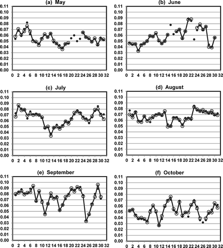
The fidelity of individual I-Bot imputed values for daily maximum 8-hr ozone is illustrated by example in for data at the Fresno-First Street monitoring site in the May–October ozone season of 2011. The 184 imputed values were based on six different Buddy Sites: Clovis (7 km, 69 days), Fresno-Drummond (9 km, 42 days), Sierra Skypark (12 km, 36 days), Madera (23 km, 26 days), Parlier (32 km, 1 day), and Visalia (66 km, 10 days). The best Buddy Site connections differed by month: Clovis dominated in June and July, Madera was common in May and October, Drummond was prevalent in August, Sierra Skypark was common from the end of August through the middle of October, and Visalia covered the final week of October. The 184 imputed values for ozone at Fresno-First Street in 2011 had mean bias of 0.2 ppb and mean error of 2 ppb. The 20 highest ozone days had mean bias of −0.3 ppb, and mean error of 3 ppb, whereas the 20 lowest ozone days had mean bias of 0.4 ppb and mean error of 2 ppb.
Figure 2. Observed values (large open circles) and imputed values (small filled circles) for daily maximum 8-hr ozone (ppm) at the Fresno-First Street monitoring station during the May–October ozone season of 2011.
The I-Bot exercise that produced the imputed values for ozone at Fresno-First Street was done for 295 monitoring sites from 1996 through 2012, using six passes through the data. shows the controls that governed I-Bot operations in each of the six passes. In most cases, observed values were available to compare with the imputed values. The final combined data set contained 1,030,670 observed values that were augmented with 272,887 imputed values. A subsequent I-Bot exercise for ozone had 363 sites from 1996 through 2013 and used minimum correlations of 0.95, 0.95, 0.90, 0.90, and 0.90 for the first five passes through the data. In that exercise, the final combined data set contained 1,114,646 observed values that were augmented with 300,205 imputed values.
The overall statewide performance of the I-Bot exercise that imputed values for daily maximum 8-hr ozone at 295 monitoring sites in California for the May–October ozone seasons from 1996 through 2012 is summarized in . The figure shows the mean bias was almost always between −2 and +2 ppb, the mean error was almost always less than or equal to 5 ppb, and the correlations between observed and imputed values were almost always greater than 0.8.
Figure 3. Performance metrics for California statewide imputations of daily maximum 8-hr ozone at 295 monitoring sites in May–October from 1996 to 2012: (a) mean bias (ppm), (b) normalized mean bias (%), (c) mean error (ppm), (d) normalized mean error (%), and (e) correlation between observed and imputed values.
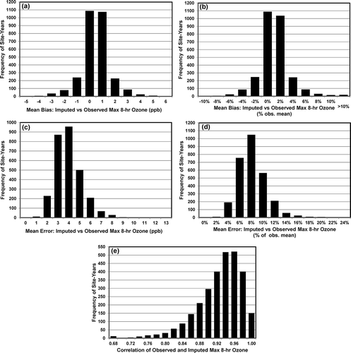
Figure 4. Observed values (large open circles) and imputed values (small filled circles), when current year data are excluded, for daily maximum 8-hr ozone (ppm) at the Fresno-First Street monitoring station during the May–October ozone season of 2011.
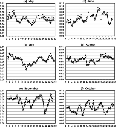
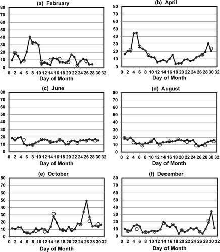
Figure 5. Observed values (large open circles) and imputed values (small filled circles) for 24-hr PM2.5 (μg/m3) at the Pasadena-Wilson monitoring station for even-numbered months in 2007.
A second I-Bot exercise imputed values for daily maximum 8-hr ozone for the full data set (295 sites from 1996 to 2012) as if each imputed value was in the middle of a full year of missing data. This was done by changing the “days to exclude (from the current year)” control from ±1 to ±15. The results for the Fresno-First Street monitoring site in the May–October ozone season of 2011 are shown in . is comparable to , showing the observed and imputed values for daily maximum 8-hr ozone. The figure reveals a noticeable positive bias until the middle of June, as Buddy Site data shifted with respect to the Target Site. The Buddy Sites used before mid-June were Fresno-Drummond and Sierra Skypark. From mid-June through October, Clovis was used as the Buddy Site. The observed bias through mid-June could be the result of different rates of instrument drift, different times of instrument recalibration, different changes in near-field emissions, and possibly other factors. Comparing with shows that the I-Bot method naturally compensates for drift, recalibration, or changes in local emissions when data are available for both the Target Site and the Buddy Site during the seasonal window in the current year.
24-Hour average PM2.5
Measured and imputed values for 24-hr average PM2.5 (a.k.a., PM-fine or fine particulate matter) for even-numbered months in 2007 are shown in during 2007 at the Wilson Avenue monitoring station in Pasadena. A Federal Reference Method (FRM) monitor measured PM2.5 on a 1-in-3-day sampling schedule at Pasadena and collected more than 100 samples. Almost all of the I-Bot imputed values were calculated using Buddy Sites at LA-North Main Street (12 km, 93 days), Burbank (18 km, 64 days), and Azusa (19 km, 193 days). The other 15 days were imputed using four other Buddy Sites. Of the three primary Buddy Sites, Azusa was used most often from 1999 through 2007. Since 2007, LA-North Main and/or Burbank have been used more frequently than Azusa. The 365 imputed values for PM2.5 at Pasadena in 2007 have mean bias of 0.6 μg/m3 and mean error of 2.4 μg/m3.
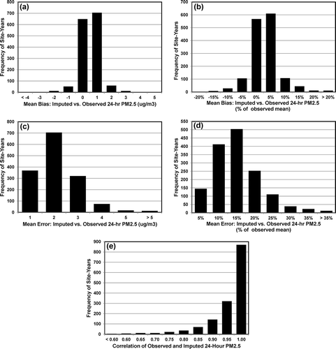
The overall statewide performance of I-Bot imputed values for 24-hr PM2.5 at 237 monitoring sites in California from 1999 through 2011 is summarized in . The figure shows the mean bias was almost always between −2 and +2 μg/m3, the mean error was almost always less than or equal to 4 μg/m3, and the correlations between observed and imputed values were almost always greater than 0.8.
Figure 6. Performance metrics for California statewide imputations of 24-hr average PM2.5 at 237 monitoring sites from 1999 to 2011: (a) mean bias (μg/m3), (b) normalized mean bias (%), (c) mean error (μg/m3), and (d) normalized mean error (%), and (e) correlation between observed and imputed values.
Mid-day average temperature
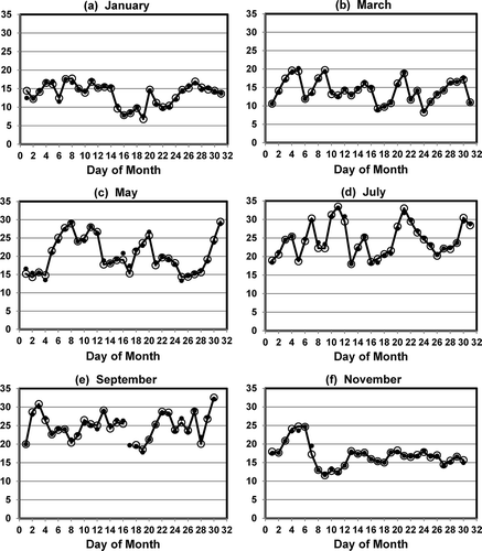
The relationship of observed to imputed mid-day average temperatures (10 a.m. to 4 p.m.) is illustrated by example in . The figure shows observed and imputed values for the Pleasanton meteorological station during odd-numbered months in 2012. The 366 imputed values for the year were based on three different Buddy Sites: Livermore Municipal Airport (10 km, 210 days), Livermore-Rincon (13 km, 100 days), and Sunol-Calaveras Road (18 km, 56 days). The mean bias of the imputed values was 0.006 °C, and the mean error was 0.5 °C.
Figure 7. Observed values (large open circles) and imputed values (small filled circles) for mid-day (10 a.m. to 4 p.m.) average temperature (°C) from 10 a.m. to 4 p.m. (PST) at Pleasanton for odd-numbered months in 2012.
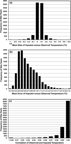
The overall statewide performance of I-Bot imputed values for mid-day average temperatures at 975 monitoring sites in California from 1996 through 2012 is summarized in . The figure shows the mean bias was almost always between −0.2 and +0.2 °C, the mean error was almost always less than or equal to 1.3 °C, and the correlations between observed and imputed values were almost always greater than 0.95.
Mid-day average wind speed
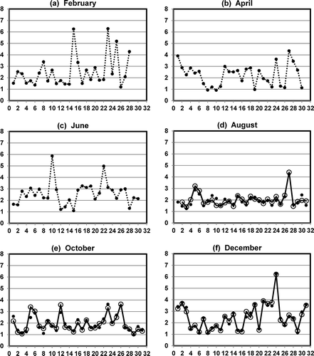
Imputing wind speed data is more difficult than imputing temperature data for multiple reasons. First, instruments that measure wind speed are often relatively less sensitive compared with those that measure temperature. Second, wind data from some sites represent full hourly average conditions, whereas data from other sites may represent as few as a single short observation per hour. And third, wind data can be relatively more variable over short distances compared with some other environmental parameters. Due to these limitations, I-Bot was able to impute mid-day average wind speeds for only 49% of the days with observed data. In contrast, I-Bot imputed mid-day average temperatures on almost 100% of the days with observed data.
presents the observed and imputed mid-day average wind speeds for even-numbered months in 2012 at the 13th&T Streets monitoring site in Sacramento. For this site in 2012, observed data were missing from January 1 through July 31. In addition, data were missing back to September 22, 2009. Because highly correlated Buddy Sites continued to measure data during this extended period of missing data, imputed values were calculated for all 365 days in 2012. In , the imputed values for February, April, and June are connected by a fine dashed line for visual convenience. A full year of differences between observed and imputed values surrounding the extended period of missing data was constructed using data from January 1, 2009, through December 31, 2012. For this period, the mean bias was −0.003 m/sec, and the mean error was 0.23 m/sec, lending credibility to the large block of imputed values.
Figure 9. Observed values (large open circles) and imputed values (small filled circles) for mid-day (10 a.m. to 4 p.m.) average wind speed (m/sec) at 13th&T Streets, Sacramento, for even-numbered months in 2012.
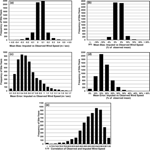
The overall statewide performance of I-Bot imputed values for mid-day average wind speed at 955 monitoring sites in California from 1996 through 2012 is summarized in . The figure shows the mean bias was almost always between −0.3 and +0.3 m/sec, the mean error was almost always less than or equal to 1.1 m/sec, and the correlations between observed and imputed values were almost always greater than 0.80.
Figure 10. Performance metrics for California statewide imputations of mid-day (10 a.m. to 4 p.m.) average wind speed at 955 monitoring sites from 1996 to 2012: (a) mean bias (m/sec), (b) normalized mean bias (%), (c) mean error (m/sec), (d) normalized mean error (%), and (e) correlation between observed and imputed values.
Alternative methods within the I-Bot approach
An alternative selection criterion
The current implementation of the I-Bot approach at CARB selects the Buddy Site for which the data have the largest correlation with the Target Site data. A better selection criterion is the smallest SEP, the estimated prediction error, that also satisfies an upper limit. We intend to alter our I-Bot system in the future to use an SEP criterion.
Alternative calculation methods
The current implementation of the I-Bot approach at CARB uses simple regression (single predictor variable). Although simple regression performs rather well, other calculation methods, such as multiple regression (multiple predictor variables) or regression models fitted with the EM algorithm might produce imputed values with better overall properties. These calculation methods would still be applied to context-intensive subsets of the data, similar to the current I-Bot approach. In section 4 of his paper, Schneider discussed ways of arranging data that would allow his approach using ridge regression with the EM algorithm to exploit patterns of spatial and temporal covariation by fitting the ridge-regression models to appropriate subsets of the data. Our context-intensive approach for I-Bot is similarly engineered to exploit patterns of spatial and temporal covariation that naturally occur in data from networks of environmental monitors.
Selected examples
The following examples involve two real-world situations in which missing data would cause difficulties. In both cases, the chief benefits of the imputed values are greater convenience and greater confidence. Greater convenience accrues because the default mode for many statistical analysis packages is to exclude records with incomplete data, and users may lack the training or experience needed to use options that permit analysis of incomplete data. And, greater confidence emerges when imputed values are credible enough to substantially reduce uncertainties regarding the effects of the missing data.
Ambient exposures to PM2.5
Epidemiological studies of acute health effects due to air pollutants may rely on daily ambient measurements. If such a study were to consider PM2.5 exposures in the South Coast Air Basin in 2013, the data for the monitoring station at Pasadena would present a significant problem. For Pasadena in 2013, no measured PM2.5 data are available for the first 5 months. CARB’s I-Bot system used Buddy Site relationships between Pasadena and sites in Los Angeles, Burbank, and Azusa to impute PM2.5 values for all 151 days. The imputed values ranged from 0 to 36.4 μg/m3, with estimated standard errors from 0.4 to 3.0 μg/m3.
Analysis of meteorological effects on ozone in the San Joaquin Valley
Surface temperature is among the key meteorological indicators of high ozone-forming potential (Rao and Zurbenko, Citation1994). Ongoing assessments of annual ozone-forming potential in major California air basins rely, in part, on daily surface temperature data. In the San Joaquin Valley, the 8-hr ozone design site for 2009 was missing mid-day temperature data from September 4 to October 28. I-Bot imputations filled in the 55 missing temperature values that ranged from 17 to 35 °C and had estimated standard errors from 0.3 to 0.5 °C. The simplest available alternatives were to use daily regional averages based on inconsistent sets of sites or to ignore all temperature data from this important site. Both of those alternatives would lead to increased uncertainty.
Conclusions
I-Bot is an effective method of imputing missing values from many networks of environmental monitors. Examples using ozone, particulate matter, temperature, and wind speed illustrate the flexibility, good precision, and high accuracy of data imputed with I-Bot. I-Bot is especially useful when the measured data include long periods (weeks, months, or years) with missing values at one or more sites. The combined data sets facilitate analysis and can help to advance scientific understanding that promotes sound policies.
Additional information
Notes on contributors
Lawrence C. Larsen
Lawrence C. Larsen is a staff air pollution specialist at the California Air Resources Board in Sacramento, CA.
Mena Shah
Mena Shah is a manager at the California Air Resources Board in Sacramento, CA.
References
- California Air Resources Board. 2006. Central California Ozone Study, Contract 05-01: Data validation. www.arb.ca.gov/airways/ccos/ccos.htm ( accessed August 20, 2015).
- Junninena, H., H. Niskaa, K. Tuppurainenc, J. Ruuskanena, and M. Kolehmainena. 2004. Methods for imputation of missing values in air quality data sets. Atmos. Environ. 38:2895–2907. doi:10.1016/j.atmosenv.2004.02.026
- Le, H.Q., S. Batterman, and R. Wahlb. 2007. Reproducibility and imputation of air toxics data. J. Environ. Monit. 9:1358–1372. doi:10.1039/b709816b
- Plaia, A., and A.L. Bondi. 2006. Single imputation method of missing values in environmental pollution data sets. Atmos. Environ. 40:7316–7330. doi:10.1016/j.atmosenv.2006.06.040
- Rao, S.T., and I.G. Zurbenko. 1994. Detecting and tracking changes in ozone air quality. J. Air Waste Manage. Assoc. 44:1089–1092. doi:10.1080/10473289.1994.10467303
- Schneider, T. 2001. Analysis of incomplete climate data: Estimation of mean values and covariance matrices and imputation of missing values.J. Climate 14:853–871. doi:10.1175/1520-0442(2001)014<0853:AOICDE>2.0.CO;2
- Triola, M.F. 2014. Elementary Statistics, 12th ed. New York: Addison-Wesley.
- U.S. Environmental Protection Agency. 2007. Guidance on the Use of Models and Other Analyses for Demonstrating Attainment of Air Quality Goals for Ozone, PM2.5, and Regional Haze. EPA-454/B-07-002. Washington, DC: U.S. Environmental Protection Agency.
- U.S. Environmental Protection Agency. 2012. Data validation: Level III. www.epa.gov/ttnamti1/files/2012conference/1A01datapreparation.pdf ( accessed August 20, 2015).

