A copula-based chance-constrained waste management planning method: An application to the city of Regina, Saskatchewan, Canada

ABSTRACT

This study proposes a copula-based chance-constrained waste management planning (CCWMP) method. The method can effectively reflect the interactions between random parameters of the waste management planning systems, and thus can help analyze the influences of their interactions on the entire systems. In particular, a joint distribution function is established using preestimated marginal distributions of random variables and an optimal copula selected from widely used Gaussian, Student’s t, Clayton, Frank, Gumbel, and Ali-Mikhail-Haq copulas. Then a set of joint probabilistic constraints in the chance-constrained programming problems is converted into individual probabilistic constraints using the joint distribution function. Further, this method is applied to residential solid waste management in the city of Regina in Canada for demonstrating its applicability. Nine scenarios based on different joint and marginal probability levels are considered within a multiperiod and multizone context to effectively reflect dynamic, uncertain, and interactive characteristics of the solid waste management systems in the city. The results provide many decision alternatives under these scenarios, including cost-effective and environmentally friendly decision schemes. Moreover, the results indicate that even though the effect of the joint probability levels on the system costs is more significant than that of the marginal probability levels, the effect of marginal probability levels is notable, and there exists a trade-off between the total system cost and the constraint-violation risk. Therefore, the results obtained from the present study would be useful to support the city’s long-term solid waste management planning and formulate local policies and regulation concerning the city’s waste generation and management.Implications: The CCWMP method not only can solve chance-constrained problems with unknown probability distributions of random variables in the right-hand sides of constraints, but also can effectively reflect the interactions between the random parameters and thus help analyze the influences of their interactions on the entire systems. The results obtained through applying this method to the city of Regina in Canada can provide many decision alternatives under different joint probability levels and marginal probability levels, and would be useful to support the city’s long-term solid waste management planning.

Introduction

The municipal solid waste (MSW) management remains a major challenge for urban policymakers and planners, due to the rising waste generation rates with the population growth and economic development, shrinking waste disposal capacities, growing environmental and health concerns, and changing legislative and political conditions (Guerrero et al., 2013; Ben-Awuah et al., 2015; Blanchard et al., 2015; Jia et al., 2015; Li et al., 2015). The MSW management mainly involves various activities associated with generation, collection, transportation, processing and disposal of solid wastes (Gunalay et al., 2012). No matter what techniques are used in these activities, MSW has to be transported from the urban areas to waste processing facilities. Since the costs of waste transportation and treatment dominantly account for operating budgets for MSW management, identification of optimal waste-flow-allocation patterns with a minimized system cost is an important task of MSW management planning (Huang et al., 2002; Wilson, 1985; Li et al., 2015). In the MSW management systems, uncertainties exist in many components and parameters, and are presented as interval, fuzzy, and/or probability formats (Wang et al., 2011; Li and Huang, 2010, 2006). Such uncertainties may be further multiplied in the waste management systems due to their multiperiod, multilayer, and multiobjective features, and may further amplify system complexities (Baets, 1990; Thomas et al., 1990). Consequently, effective methods are desired to reflect extensive uncertainties in the MSW management systems and to establish effective waste-flow allocation patterns under an uncertain environment (Chang and Wang, 1993; Zhu and Revelle, 1993; Li and Huang, 2010, 2006).

An effective approach for dealing with uncertainties in MSW management systems is the chance constrained programming (CCP) method. The CCP method can reflect the reliability of satisfying (or risk of violating) system constraints under uncertainty (Charnes et al., 1972; Charnes and Cooper, 1983; Li et al., 2009). It can be further divided into two classes of probability-constrained problems: individual probability constrained (IPC) and joint probability constrained (JPC). In the IPC problem, each of the chance constraints would be satisfied with a probability level and they must be independent of each other, whereas a whole set of chance constraints must be satisfied at a probability level in the JPC problem. In comparison with the IPC problem, the JPC problem allows analyzing interactions among multiple chance constraints, and thereby improves robustness in controlling system risk in the optimization process (Li et al., 2009; Liu et al., 2015). Therefore, the JPC approach is more suitable for dealing with such uncertainties.

In the past decade, a number of research works have been proposed to deal with uncertainties through the JPC approach. For instance, Ruszczyński (2002) developed a specialized method to deal with the JPC problems using a discrete representation obtained by Monte Carlo sampling. Sampling approximation of the JPC problems has been further studied by Calafiore and Campi (2005, 2006) and Luedtke and Ahmed (2008). However, the sampling-based approach may be computationally prohibitive to solve large-scale practical problems, and the effectiveness of sampling approximation has also been challenged (Chen et al., 2010). For the large-scale practical problems, existing methods for solving the JPC problems (An and Eheart, 2007; Xu et al., 2009, 2014; Sun et al., 2010, 2013; Lv et al., 2001; Gu et al., 2013; Liu et al., 2015) mainly transformed the chance-constrained programming problems into deterministic problems through approximating joint chance constraints by a set of individual chance constraints and a new joint constraint that the summation over all probabilities of failure of individual chance constraints is less than or equal to the joint one. However, such approximation is based on the assumptions that each of the random variables follows a specific probability distribution (e.g., Gaussian (normal), gamma, lognormal, or exponential distribution) and that all the random variables are independent to each other. However, in most real-world problems, both the probability distributions of individual random variables on the right-hand sides and the correlated nature among them are unknown. In other words, this assumption cannot often be satisfied in the real-world problems, and thus the summation over all probabilities of violation for individual chance constraints cannot be guaranteed to be less than or equal to the joint one. Nevertheless, an effective approach for solving JPC problems with unknown probability distributions of random variables in the right-hand sides and correlation relationships among them has not been reported in the literature.

The key question for solving such JPC problems is to characterize the relationship between the individual probability distributions of random variables and their joint probability distribution, which may be achieved through modeling multivariate joint distributions. Sklar proposed a “copula” approach for modeling multivariate joint distributions in 1959 (Nelsen, 2006). This approach showed that a multivariate joint distribution can be completely characterized by its respective marginal distributions and a copula function for binding them together independent of the types of individual marginal distributions. The copula approach is a useful method for deriving joint distributions given the marginal distributions, and is used to define nonparametric measures of dependence for pairs of random variables. Modeling joint distributions using copulas has a substantial advantage of allowing researchers to consider marginal distributions and dependence as two separate but related issues. Copulas have been used recently to construct multivariate models with a variety of dependence structures in the financial and actuarial fields (Mendes and Souza, 2004; Smith, 2003; Li, 2000), biostatistics (Wang and Rennolls, 2007; Wang et al., 2008; Wang, 2003; Fine and Jiang, 2000) and hydrology (Karmakar and Simonovic, 2009; Zhang and Singh, 2006; Yue and Rasmussen, 2002). However, the general concept and techniques for the practical use of copulas are new to mathematical optimization methods for environmental engineering.

Therefore, the objective of this study is to propose a copula-based chance-constrained waste management planning method and apply it to the city of Regina in Canada. The method can deal with the joint-probabilistic chance-constrained waste management planning problems having unknown probability distributions of random variables in the right-hand sides and correlation relationships among them, and can more effectively reflect interactions between the random variables. In detail, the method is to estimate marginal distribution functions of random variables based on historical data by parametric or nonparametric methods, establish a joint distribution function using a copula, and then convert joint probabilistic constraints into individual probabilistic constraints using the joint distribution function. The copula will be selected as the best one from widely used Gaussian, Student’s t, Clayton, Frank, Gumbel, and Ali-Mikhail-Haq copulas. Additionally, the application of this method to the city of Regina in Canada will demonstrate its applicability to provide useful information for supporting the city’s long-term solid waste management planning.

Chance-constrained waste management planning method

Chance-constrained waste management planning model

A chance-constrained planning model for MSW management of a city may be formulated as follows (Model A):

The objective function is

(1)

subject to:

1. Landfill capacity constraint:

   (2)

2. Composting capacity constraint:

   (3)

3. Composting capacity constraint:

   (4)

4. Waste disposal demand constraint:

   (5)
   (6)

5. Nonnegativity constraint:

   (7)

6. Binary constraint:

   (8)
   (9)

7. Landfill expansion constraints:

   (10)
   (Landfill expansion may only be considered once in the entire planning horizon.)

8. Constraints of expansions for composting and recycling facilities:

   (11)

(Expansion may only occur once for composting and recycling facilities in any given time period.)

In these equations, f is the net system cost ($); i (i = 1, 2, 3) denotes three representative solid waste management facilities, with i = 1 representing a landfill, i = 2 representing a composting facility, and i = 3 representing a recycling facility (or material recovery facility); j (j = 1, 2, …, J) denotes geographic zones of the city; k (k = 1, 2, .., K) represents time periods in the planning horizon, with each period having a fixed time length; m (m = 1, 2, …, M) denotes capacity-expansion options for the solid waste management facilities; L_k is the length of time period k (weeks); X_ijk are continuous decision variables representing the waste flow from the residences in zone j to facility i during period k (tonnes/week); TR_ijk denotes the collection and transportation cost for waste flow from the residences in zone j to facility i during period k ($/tonne); OP_ik denotes the operating cost of facility i during period k ($/tonne); FE_i denotes a ratio of the residues generated in composting or recycling facility (percent of incoming mass to facility i), i = 2, 3; FT_ik denotes the collection and transportation cost for waste flow from composting or recycling facility to the landfill during period k ($/tonne), i = 2, 3; RE_ik denotes the revenue generated by processing waste flows in composting or recycling facility during period k ($/tonne), i = 2, 3; FLC_mk denotes the capital cost for expanding the landfill by option m during k ($/tonne); Y_mk are binary decision variables for expanding the landfill by option m at the start of period k; FTC_imk denotes the capital cost for expanding composting or recycling facility by option m during k ($/tonne), i = 2, 3; Z_imk are binary decision variables for expanding composting or recycling facility by option m at the start of period k, i = 2, 3; LC denotes the existing landfill capacity (tonnes); denotes the amount of capacity expansion option m for the landfill (tonnes); TC_i denotes the existing capacity for composting or recycling facility (tonnes/week), i = 2, 3; denotes the amount of capacity expansion option m for composting or recycling facility (tonnes/week), i = 2, 3; and denotes the waste generation rate of the residences in zone j during period k (tonnes/week).

In Model A, the waste generation rates of the residences in zones j = 1, 2,…, n are random parameters with unknown distributions, whereas other parameters and coefficients are deterministic real numbers; Pr{} is the operator of probability; is a prescribed joint probability level at which the entire set of chance constraints given by formula 5 is enforced to be satisfied; and p is a prescribed probabilistic violation level for the entire set of chance constraints. The set of chance constraints means that the constraints are not required to be satisfied by 100% probability but can be violated with the maximum probability of p.

The key question for solving this model is to characterize the relationship between the individual probability distributions of random variables and their joint probability distribution, which means, for a given violation probability of constraints as in eq 5, what the individual violation probabilities would be for In general, distribution information of random variables can be obtained from historical data. The procedure of obtaining the joint probability distribution from historical data is very complicated, especially when the random variables follow different marginal probability distributions. In this study, we use a “copula” function to model a joint probability distribution of the random variables , so that distribution information on the random variables can be effectively and simply obtained. Thus, a brief introduction of copulas is presented next.

Brief introduction of copulas

The “copula” approach for modeling multivariate joint distributions was proposed by Sklar in 1959 (Nelsen, 2006). This approach showed that a multivariate joint distribution can be completely characterized by its respective marginal distributions and a copula function for binding them together independent of the types of individual marginal distributions. The copula approach is a useful method for deriving joint distributions given the marginal distributions, and is used to define nonparametric measures of dependence for pairs of random variables. Modeling joint distributions using copulas has a substantial advantage of allowing researchers to consider marginal distributions and dependence as two separate but related issues. Copulas have been used recently to construct multivariate models with a variety of dependence structures in the financial and actuarial fields (Mendes and Souza, 2004; Smith, 2003; Li, 2000), biostatistics (Wang and Rennolls, 2007; Wang et al., 2008; Wang, 2003; Fine and Jiang, 2000), and hydrology (Karmakar and Simonovic, 2009; Zhang and Singh, 2006; Yue and Rasmussen, 2002). However, the general concept and techniques for the practical use of copulas are new to mathematical optimization methods for environmental engineering.

Several bivariate copulas to be applied in a case study are briefly introduced next.

(1) Gaussian (normal) copula. The bivariate Gaussian copula takes the form (Trivedi and Zimmer, 2007):

(12)

where is the cumulative distribution function of the standard normal distribution, and is the standard bivariate normal distribution with correlation parameter θ restricted to the interval (–1, 1). The parameter θ measures the degree of dependence. The larger the absolute value of θ is, the stronger the dependence between variables is, where θ > 0 implies positive dependence, θ < 0 implied negative dependence, and θ = 0 implies independence.

(2) Student’s t-copula. The bivariate t-copula with k degrees of freedom and correlation parameter ρ takes the form (Trivedi and Zimmer, 2007):

(13)

where is the inverse of the cumulative distribution function of the standard univariate t-distribution with k degrees of freedom. Like the Gaussian copula, the correlation parameter ρ for measuring the degree of dependence is also restricted to the interval (–1, 1). In detail, the larger the absolute value of ρ is, the stronger the dependence between variables is, where ρ > 0 implies positive dependence, ρ < 0 implied negative dependence, and ρ = 0 implies independence.

(3) Archimedean copulas. Archimedean copulas are widely applied classes of copula functions for the ease with which they can be constructed and the nice properties they possess. In the present study, Clayton, Frank, Gumbel, and Ali-Mikhail-Haq (AMH) bivariate copulas belonging to the class of Archimedean copulas are considered for analysis. The mathematical expressions of the four bivariate Archimedean copulas and their fundamental properties are listed in Table 1. In Table 1, is the hidden parameter of the generating function called a generator, and is a continuous convex function decreasing from to (Karmakar and Simonovic, 2009).

Table 1. Selected bivariate Archimedean copulas.

Copula family		Range of	Generating function*[]
Clayton
Frank
Gumbel
Ali-Mikhail-Haq (AMH)

Archimedean copulas can be determined by the following steps: estimating Kendall’s coefficient () from the observed data; determining the parameter from the estimated Kendall’s coefficient () for each of the copulas given in Table 1; obtaining the generating function of each copula; and obtaining the copulas from their generating functions (Karmakar and Simonovic, 2009).

Proposed solution

In general, the proposed solution for Model A is to (i) convert the joint chance constraints of eq 5 into individual chance constraints, which are presented in Figure 1, and (ii) transform an individual chance constrained problem to an equivalent linearly constrained problem, which will substantially be the same as in the previous studies. In detail, a deterministic programming model can be obtained finally and solved by traditional optimization methods. For the ease of description, we take the number of random variables being 2 (i.e., n = 2) as an example to illustrate the process of (i) with reference to Figure 1.

Figure 1. Schematic diagram of proposed solution method.

First, the marginal cumulative distributions can be estimated by parametric or nonparametric estimation methods known from the statistical literature (Akaike, 1974; Scott, 1992, 2001; Silverman, 1986). Since the nonparametric method gives more accurate results than parametric methods, a nonparametric method based on kernel density estimation will be used to estimate the nonparametric marginal distribution functions for random variables (hereafter referred to as ). It is assumed that each of the random variables has historical data of N observations, that is, . The probability density function f_l(x) and cumulative distribution function F_l(x) of each random variable at x may be estimated by the following formulas:

(14)

(15)

(16)

(17)

where N is the number of observations, x_j is the jth observation, h is the smoothing parameter known as “bandwidth,” , S is the sample standard deviation, and IQR is the interquartile range (Akaike, 1974; Scott, 1992, 2001; Silverman, 1986). The kernel density estimation method is computationally simple, but it may appear less efficient when there are fewer available data. To overcome the drawback of kernel density estimation method, an orthonormal series method may be used to estimate marginal distribution functions for random variables from the historical data (Bowman and Azzalini, 1997; Efromovich, 1999). In the present study, Kolmogorov–Smirnov, Anderson–Darling, and Cramér–von Mises statistic tests are used to evaluate goodness of fit for the marginal cumulative distribution functions (Anderson and Darling, 1952; Choulakian et al., 1994; Stephens, 1974).

Different classes of copulas are used to generate joint distribution functions with different dependence structures (Nelsen, 2006). Since each class of copula restricts the dependence structure, no single copula will work well in all data situations. The Gaussian copula is the traditional and simple candidate for modeling dependence. Student’s t copula can describe dependence in the tails while keeping flexibility of establishing dependence in the center. Clayton, Frank, Gumbel, and Ali-Mikhail-Haq copulas are four classes of Archimedean copulas widely applied in the practice problems for their many nice properties. Thus, we consider Gaussian, Student’s t, Clayton, Frank, Gumbel, and Ali-Mikhail-Haq (AMH) copulas to model the dependence therein.

After classes of copulas to be considered are selected, we need to determine copula parameter for each class of copula now. Suppose that we use a specific copula with cumulative distribution function C and parameter to model the dependence of random variables from N observations. Generally, there are two methods for estimating the copula parameter . A first method is simultaneous estimation of all parameters using the full maximum likelihood (FML) approach, which is the most direct estimation method. Another method is a sequential two-step maximum likelihood method (TSML) where the marginal parameters are estimated in the first step and the dependence parameters in copulas are estimated in the second step (Joe, 1997). Because the TSML approach enables us to explicitly isolate the dependency modeling from fitting individual marginal distributions, we would consider adopting the TSML approach to estimate the parameter . Once the copula parameter is determined, a corresponding copula function can be generated based on the determined parameter and a joint cumulative distribution function may be obtained using the copula function. Next, we test the goodness of fit of observed data to the theoretical joint cumulative distributions obtained using copula functions by the root mean square error (RMSE), Akaike information criterion (AIC), and Bayesian information criteria (BIC) (Karmakar and Simonovic, 2009).

1. RMSE is expressed as:

(18)

where N is the number of observations; k is the number of fitted parameters; P_c is the theoretical joint distribution frequency obtained using copula functions; and P_o is the empirical joint distribution frequency given by

(19)

where n_ml is the number of pairs (x_j,y_j) counted as and , , and N is the sample size.

1. AIC is expressed as:

(20)

where N is the number of observations; ; and k is the number of fitted parameters.

1. BIC is expressed as:

(21)

where N is the number of observations; ; and k is the number of fitted parameters.

The best copula is the one that has the minimum RMSE, AIC, and BIC values. More details of the goodness-of-fit tests for copulas are given in Panchenko (2005) and Genest et al. (2007).

We can obtain the joint cumulative distribution function (CDF) of random variables from the selected best copula using , where and are the inverse of the marginal cumulative distribution function of random variables and , respectively.

Bayes’s Rule states the following:

(22)

where P(B/A) is the conditional probability that B occurs given that A has occurred, and is the joint probability that A and B occur together. This rule also shows that the unconditional probability that A occurs is the conditional probability multiplied by the joint probability. According to Bayes’s rule, a conditional CDF of given is expressed as

(23)

where is the joint CDF of random variable X and Y; and is the marginal CDF of random variable Y.

It can be seen from the relationship among the joint, conditional, and marginal CDF that the marginal CDF can be determined from the joint CDF when the conditional CDF is given. Based on this property, constraints of eq 5 in Model A can be rewritten as

(24)

(25)

where is a probabilistic violation level for the jth individual chance constraint, also known as a significance level representing the acceptable risk of constraint violating; p is the probabilistic violation level for eq 5, and is the best copula determined previously.

According to the chance-constrained programming method proposed by Charnes et al. (1972), when the left-hand-side coefficients are deterministic and the right-hand-side coefficients are random, the constraints of eq 24 can be transformed as

(26)

where ; is a probabilistic violation level for the jth individual chance constraint; and is the inverse CDF of the jth random variable. As a result, Model A will become a general linear programming problem with constraints of eqs 25 and 26 instead of eq 5, which may be solved by commercial software such as LINDO or LINGO.

Case study

Overview of study system

The chance-constrained waste management planning method will be demonstrated through residential solid waste management in the city of Regina, Canada, the geographic map of which is presented in Figure 2 (Canada Map, 2015). The city of Regina is the provincial capital of Saskatchewan with a population of 244,000 within the city limits, and the average annual growth rate is estimated to be 2.8% based on the population status over the last 5 years (City of Regina, 2014; Regina Regional Opportunities Commission, 2015). The Community Association & Zone Map of the City of Regina is displayed in Figure 3 (City of Regina, 2014). As shown in Figure 3, the city of Regina consists of five zones, namely, the central zone, west zone, east zone, south zone, and north zone, and the five zones are in turn made up of 28 community associations.

Figure 2. Geographic map of Canada showing Canadian provinces and provincial capitals.

Figure 3. Community Association & Zone Map of the city of Regina.

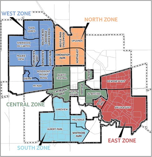
The city of Regina provides residential solid waste services to more than 65,000 residences (City of Regina, 2009). The residential solid waste services include waste collection, waste diversion, waste recycling and composting, landfill disposal, and other related services. Currently, the residential services are very economical, costing about $110/household/year, and the residential satisfaction is very high for basic garbage services (City of Regina, 2012). For the waste collection, the city of Regina employs the residential automated front of street collection (approximately 57% residents receiving this service) and residential mechanical collection (approximately 43% residents receiving this service) to collect the residential garbage once per week (City of Regina, 2013). The collected solid wastes typically include paper, plastic, glass, cardboard, metal (ferrous and nonferrous), hygienic waste, meat organics, yard waste, household hazardous waste, and other wastes (City of Regina, 2009). The city of Regina landfill is the only landfill in the Regina area, and is located on Fleet Street in the city’s northeast quadrant. All solid wastes not diverted in the Regina area are disposed of at the landfill. Approximately 65,000 tonnes/year of residential solid waste is buried at the landfill. The current landfill (its capacity was expanded once in 2010) is expected to reach capacity within 20 years based on the current waste generation rates in the city of Regina (City of Regina, 2014). However, with the population growth and economic development, the waste generation rates in the city of Regina increase rapidly. Thus, the landfill will confront such a problem in that its capacity may be insufficient to meet the overall waste disposal demand in the next 25 years. In this case, the capacity expansion for the landfill will be needed to satisfy the rising demands for waste disposal. Due to the scarcity of land around the urban center and the growing opposition from the public with regard to landfill operation, the city council is making efforts toward waste diversion through an integrated solid waste management plan for collection and disposal of waste, to change the current practice of relying solely on the landfill for its waste disposal (City of Regina, 2014). The city of Regina established a 20-year solid waste management strategy to achieve a solid waste diversion rate goal of 50% or higher in 2025 (City of Regina, 2009). The city provides a variety of waste diversion programs, including residential curbside recycling collection, a backyard composting program, a national stewardship program for used batteries, household hazardous waste events, and so on (City of Regina, 2014). The residents are receiving curbside collection of their recyclable and backyard waste, and a diversion rate of 19% is achieved through various landfill diversion options such as Regina’s residential recycling service and backyard composting programs (City of Regina, 2013). In order to prolong the life of the landfill, a higher diversion rate (particularly at least 30%) could be expected.

Presently, the city of Regina employs the landfill, recycling, and composting (backyard) facilities for managing its residential solid waste (City of Regina, 2014). In detail, the city’s residential waste management system involves garbage collection from the residences in the five zones, waste transportation to the recycling facility, composting facility, or landfill, waste recovery, organic waste composting, and waste disposal. Since the city’s population keeps growing and the living standard of the people continues to improve with the economic development, the waste generation rates in the city increase accordingly. When the existing capacities of the landfill, recycling, and composting facilities are inadequate to satisfy the increasing waste management demands of the city, it will be necessary to make capacity expansions for these waste management facilities (City of Regina, 2013). Since the relationships between waste generation and available capacities of these facilities are temporally varied, the optimal schemes for effective utilization of the facilities (i.e., optimal waste flow allocation patterns) will also vary over time. In implementing the integrated waste management plan within a multiperiod and multizone context, many impact factors and their interactions should be systematically evaluated. In detail, the following challenging issues are desirable to be addressed: (1) What is the least-cost means for achieving the diversion rate goal under uncertainty? (2) When and what kind of capacity expansion would the landfill, the recycling, and the composting facilities undertake during the next 25-year period? (3) What would the optimal waste flow allocation patterns be in different time periods? (4) How would we effectively use the waste management facilities to prolong the landfill’s life?

Additionally, the waste generation has temporal and spatial variations due to variations of the population growth and economic development in different zones. Moreover, one cannot exactly predict the waste generation in the future. Thus, in the city’s waste management planning system, the waste disposal demand will be uncertain. As stated previously, the joint chance-constrained programming method is an effective and robust approach for dealing with such uncertainties.

Chance-constrained programming model for the city’s waste management planning

To address the issues already mentioned, a joint-probabilistic chance-constrained programming (JCCP) model is developed for supporting the city’s residential waste management planning. The results are expected to provide useful information for supporting the city’s long-term solid waste management planning, and formulating local policies and regulations concerning the city’s waste generation and management.

A planning horizon to be studied here is 25 years (i.e., 2016 to 2040), with five periods each having a time interval of 5 years. The landfill directly receives the residential solid wastes from the five zones and the residues from the recycling and composting facilities. It is often used to meet the waste disposal demands, and is characterized by an overall capacity limit. The recycling facility is used to recycle solid wastes with a ratio of the residues being 15%, the composting facility is used to compost organic wastes with a ratio of the residues being 10%, and the two facilities are characterized by a weekly operating capacity limit (city of Regina, 2013). The existing capacity of the landfill for the residential solid waste is roughly estimated to be 800,000 tonnes, and the existing capacities of the recycling and composting facilities for the residential solid waste are 250 tonnes/week and 150 tonnes/week, respectively (City of Regina, 2012). There will be potentially three expansion options for each of the landfill and recycling and composting facilities to be considered for the whole planning horizon.

The JCCP model for the city’s waste management planning aims to minimize the total system cost by achieving optimal waste flow allocation patterns and optimal plans for the facilities’ capacity expansion over the entire planning horizon. The JCCP model is given by eqs 1 to 11 presented in the “Chance-constrained waste management planning model” section, where j (j = 1, 2, 3, 4, 5) denotes five community zones in the city of Regina, with j = 1 representing central zone, j = 2 representing west zone, j = 3 representing east zone, j = 4 representing south zone, j = 5 representing north zone; k (k = 1, 2, 3, 4, 5) representing five time periods in the planning horizon with 25 years, each period having 5 years; m (m = 1, 2, 3) denoting three capacity-expansion options for each of the solid waste management facilities; and n (n = 2) meaning that only the waste generation rates for central zone and west zone are random variables with unknown probability distributions.

It should be noted that we have made the following assumptions during formulating the JCCP model: (i) All residential solid wastes generated within a certain period must be timely shipped to a disposal site after their generation without any mass loss in the transportation process; (ii) capacity expansion of any waste management facility within a certain period should be completed at the start of this period; (iii) the waste management system only considers the residential solid wastes generated in the city’s households, because the waste management for industrial, commercial, and institutional wastes from nonresidential sectors is not under the supervision of the municipal government; and (iv) since the waste generation is proportional to the population and the average living standards or the average income of the people, the waste generate rates ω_jk for central and west zones j = 1, 2 increase with a fixed annual growth rate of 2.8% (which is determined based on the average growth rate of the city’s population and gross domestic product [GDP] per capita in the past 5 years) over the next 25 years.

Data collection and utilization

Table 2 presents the waste generation rates of the east zone, south zone, and north zone, operating costs, capacity expansion options and relevant capital costs for three waste management facilities, collection and transportation costs for waste flows, and revenues from recycling and composting facilities over the five planning periods (City of Regina, 2009, 2012, 2013, 2014). The waste generation rates for the central zone and west zone are random variables with unknown probability distributions. In this case study, 5 years (2009 to 2014) of weekly waste generation data is used to determine the respective marginal cumulative distribution functions of the random variables and a joint cumulative distribution function for measuring statistical dependence between them.

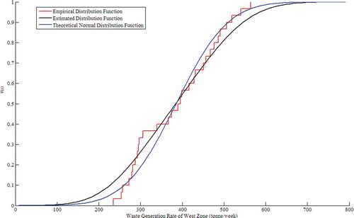
On the basis of the procedures explained in the “Chance-constrained waste management planning method” section, comparisons of empirical distribution functions, estimated distribution functions using the kernel estimation method, and theoretical normal distribution functions for the waste generation rates of the central zone and west zone are shown in Figures 4 and 5, respectively. It can be seen from Figures 4 and 5 that the waste generation rates of the two zones have marginal distributions of normal distribution functions, which is consistent with the assumption that random parameters follow normal distributions in the previous studies for municipal waste management. Moreover, the Kolmogorov–Smirnov, Anderson–Darling, and Cramér–von Mises statistic tests confirm that they are normally distributed. However, Kendall’s coefficient of correlation (t), Pearson’s linear correlation coefficient (ν,) and Spearman’s correlation coefficient (ρ) are –0.1448, –0.3062, and –0.2743, respectively, which indicates that they are mutually correlated. Using the TSML approach, we can obtain the copula parameters (θ) of Archimedean copulas mentioned earlier, shown in Table 3.

Table 2. Waste-generation rate, costs, revenues and capacity expansion options and their capital costs for waste management facilities.

	Planning period
	k = 1	k = 2	k = 3	k = 4	k = 5
Waste-generation rate, (tonne/week)
East zone, j = 3	404.94	449.63	496.38	545.47	607.24
South zone, j = 4	377.68	431.36	466.94	524.72	564.98
North zone, j = 5	363.36	392.23	422.34	493.87	507.01
Operation costs of waste management facilities, OPik ($/tonne)
Landfill, i = 1	36.49	33.40	29.33	26.53	22.12
Composting facility, i = 2	51.61	44.31	35.56	27.34	24.66
Recycling facility, i = 3	66.62	56.37	46.15	37.50	36.19
Residue costs, FTik ($/tonne)
Composting, i = 2	2.54	1.95	1.65	1.39	1.18
Recycling, i = 3	2.12	1.63	1.37	1.16	0.98
Revenues from waste management facilities, REik ($/tonne)
Composting facility, i = 2	10.09	7.73	6.54	5.53	4.68
Recycling facility, i = 3	51.20	46.88	43.59	41.53	37.25
Collection and transportation costs, TRijk ($/tonne)
From central zone to landfill, i = 1, j = 1	38.39	34.1	32.47	31.24	27.47
From west zone to landfill, i = 1, j = 2	51.98	50.20	42.49	36.43	33.46
From east zone to landfill, i = 1, j = 3	24.59	32.09	20.80	14.90	17.60
From south zone to landfill, i = 1, j = 4	59.37	53.16	44.38	35.23	27.08
From north zone to landfill, i = 1, j = 5	49.19	46.59	41.60	37.79	35.20
From central zone to composting facility, i = 2, j = 1	37.16	42.26	34.94	30.74	44.33
From west zone to composting facility, i = 2, j = 2	55.12	53.54	49.77	45.96	40.43
From east zone to composting facility, i = 2, j = 3	32.52	42.45	27.51	19.70	23.27
From south zone to composting facility, i = 2, j = 4	54.38	47.86	43.19	41.16	35.55
From north zone to composting facility, i = 2, j = 5	60.89	57.04	55.02	46.55	39.38
From central zone to recycling facility, i = 3, j = 1	62.23	58.06	51.42	46.53	42.27
From west zone to recycling facility, i = 3, j = 2	56.76	54.37	50.97	47.33	45.33
From east zone to recycling facility, i = 3, j = 3	44.99	42.73	38.06	35.25	32.21
From south zone to recycling facility, i = 3, j = 4	66.58	62.45	56.89	52.68	49.47
From north zone to recycling facility, i = 3, j = 5	70.78	69.45	60.14	54.49	56.41
Capacity expansion options and corresponding capital costs ($10^8)
Landfill (FLCmk)
m = 1,	7.84	6.70	5.73	4.87	4.14
m = 2,	10.70	9.03	7.74	6.59	5.62
m = 3,	12.60	10.80	9.13	7.78	6.70
Composting facility (FTC2mk)
m = 1,	0.85	0.73	0.62	0.53	0.45
m = 2,	1.70	1.45	1.24	1.06	0.90
m = 3,	1.33	1.13	1.07	0.91	0.77
Recycling facility (FTC3mk)
m = 1,	0.87	0.74	0.63	0.54	0.46
m = 2,	1.75	1.49	1.26	1.08	0.93
m = 3,	2.14	1.81	1.56	1.33	1.14

Table 3. Copula parameters of Archimedean copulas determined using the TSML approach.

Copula	Copula parameter ()
Clayton	–0.2530
Frank	–1.3258
Gumbel	0.8735
Ali-Mikhail-Haq	0.8239

Figure 4. Comparison of empirical distribution function, estimated distribution function using the kernel estimation method and theoretical normal distribution function of N(306.68, 77.85²) for the waste generation data of the central zone.

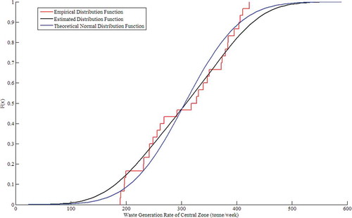
Figure 5. Comparison of empirical distribution function, estimated distribution function using the kernel estimation method and theoretical normal distribution function of N(385.33, 97.15²) for the waste generation data of the west zone.

With reference to Table 1, we can see that the parameters of Clayton and Gumbel copulas, being –0.2530 and 0.8735, respectively, are beyond the range of θ shown in Table 1, so Clayton and Gumbel copulas will be not suitable for modeling the joint distribution of the two random variables. In this case, only Gaussian, Student’s t, Frank, and Ali-Mikhail-Haq copulas may be used to model the joint distribution. The RMSE, AIC, and BIC values for joint cumulative distributions obtained using the four classes of copulas are shown in Table 4. It can be concluded from Table 4 that the Gaussian copula is the best one for modeling the joint cumulative distribution function of the two random variables, because the minimum RMSE, AIC, and BIC values are obtained for this class of copula. The joint cumulative distribution function for the waste generation rates of the central zone and west zone using the Gaussian copula is shown in Figure 6.

Table 4. Comparison of RMSE, AIC and BIC values for joint distributions using copula models.

Copula	RMSE	AIC	BIC
Gaussian	0.0345	–41.8654	–42.3883
Student’s t	0.0449	–35.0076	–35.5305
Frank	0.0400	–38.0045	–38.5273
Ali-Mikhail-Haq	0.0493	–32.5359	–33.0587

Figure 6. Joint cumulative distribution function for the waste generation rates of the central zone and west zone using the Gaussian copula.

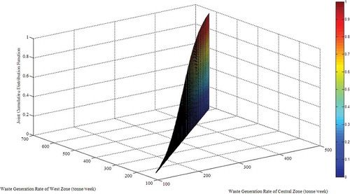
The joint cumulative distribution function for the waste generation rates of the central zone and west zone may be determined using the bivariate Gaussian copula obtained earlier as the best copula model, and Table 5 shows selected representative values of joint cumulative distribution , conditional cumulative distribution , marginal cumulative distributions and , and corresponding values of random variables X and Y under nine scenarios, where X and Y are random variables denoting the waste generation rates of the central zone and west zone, respectively. Thereafter, the nine scenarios are referred to as scenarios of constraint-violation levels being (0.1,0.09,0.008), (0.1,0.07,0.028), (0.1,0.05,0.048), (0.1,0.03,0.068), (0.1,0.01,0.088), (0.05,0.04,0.008), (0.05,0.03,0.018), (0.05,0.02,0.028) and (0.05,0.01,0.038), where denotes the joint probability levels, and and denote the marginal probability levels of random variable X and Y, respectively. In detail, we selected two joint probability levels of 0.9 and 0.95, where there were five sets of marginal probability levels at the joint probability level of 0.9, and four sets of marginal probability levels at the joint probability level of 0.95.

Based on the chance-constrained waste management planning method described previously, the joint chance constraints of eq 26 can be converted as the following individual chance constraints:

(27)

(28)

where F⁻¹() and G⁻¹() are the inverse of the marginal cumulative distribution functions F_X(x) and G_Y(y), respectively. In this case, the joint-probabilistic chance-constrained programming model for the city’s waste management planning has been converted into a general linear programming model, which may be solved by commercial software such as LINDO or LINGO.

Result analysis and discussion

Table 6 shows the optimal solution of the city’s waste management system under nine scenarios of. The results generally indicate that the optimal solutions would vary with the constraints violation levels (or the joint probability level and marginal probability levels), and the waste-flow-allocation patterns would have temporal and spatial variations under each of the nine scenarios. Meanwhile, it can be seen from Table 6 that the waste flows from the east and south zones to the three waste management facilities would be identical under the nine scenarios, the waste flows from the central and west zones to the three waste management facilities would significantly vary under different scenarios, and the waste flows from the north zone to the three waste management facilities would be slightly different under different scenarios. Since the waste generation rates of the central zone and west zone are random variables, the waste flows allocated from the two zones to the waste management facilities would be sensitive to the constraints violation levels.

Table 5. Selected values of joint cumulative distribution conditional cumulative distribution , marginal cumulative distributions and , and corresponding values of random variables X and Y.

HX,Y(x,y)	HY/X(y|X≤x)	FX(x)	GY(y)	x	y	(p,p1,p2)
0.900	0.989	0.910	0.992	411.06	619.34	(0.1,0.09,0.008)
0.900	0.968	0.930	0.972	421.57	570.98	(0.1,0.07,0.028)
0.900	0.947	0.950	0.952	434.74	547.05	(0.1,0.05,0.048)
0.900	0.928	0.970	0.932	453.11	530.17	(0.1,0.03,0.068)
0.900	0.909	0.990	0.912	487.80	516.80	(0.1,0.01,0.088)
0.950	0.990	0.960	0.992	442.98	619.34	(0.05,0.04,0.008)
0.950	0.979	0.970	0.982	453.11	589.05	(0.05,0.03,0.018)
0.950	0.969	0.980	0.972	466.56	570.98	(0.05,0.02,0.028)
0.950	0.960	0.990	0.962	487.80	557.71	(0.05,0.01,0.038)

Table 6. Solution of the waste management system.

	(p,p1,p2)	(p,p1,p2)	(p,p1,p2) =	(p,p1,p2)	(p,p1,p2)	(p,p1,p2)	(p,p1,p2)	(p,p1,p2)	(p,p1,p2)
	(0.1,0.09,0.008)	(0.1,0.07,0.028)	(0.1,0.05,0.048)	(0.1,0.03,0.068)	(0.1,0.01,0.088)	(0.05,0.04,0.008)	(0.05,0.03,0.018)	(0.05,0.02,0.028)	(0.05,0.01,0.038)
Xijk (tonnes/week)
X111	411.06	421.57	434.74	453.1	487.79	442.98	453.1	466.57	487.79
X112	429.09	440.07	453.8	472.98	509.19	462.41	472.98	487.03	509.19
X113	202.23	213.62	227.88	247.78	285.35	479.87	247.78	262.36	285.35
X114	0	0	0	0	0	119.82	0	0	0
X115	392.48	407.71	426.78	453.39	503.64	641.71	453.39	472.89	503.64
X121	147.03	268.66	244.72	227.84	44.47	199.35	116.72	98.66	85.39
X122	0	0	0	0	0	222.52	0	0	0
X123	77.24	25.13	0	0	0	247.24	44.59	25.13	10.83
X124	115.79	60.68	33.39	14.16	0	285.79	81.26	60.68	45.55
X125	138.36	81.48	53.32	33.48	17.75	308.36	102.72	81.48	65.87
X131	404.94	404.94	404.94	404.94	404.94	404.94	404.94	404.94	404.94
X132	449.63	449.63	449.63	449.63	449.63	449.63	449.63	449.63	438.2
X133	496.38	496.38	496.38	496.38	496.38	496.38	496.38	496.38	496.38
X134	545.47	545.47	545.47	545.47	545.47	545.47	545.47	545.47	545.47
X135	607.24	607.24	607.24	607.24	607.24	607.24	607.24	607.24	607.24
X141	0	0	0	0	0	19.74	0	0	0
X142	0	0	0	0	0	1.36	0	0	0
X143	0	0	0	0	0	36.94	0	0	0
X144	524.72	524.72	524.72	524.72	524.72	524.72	524.72	524.72	524.72
X145	564.98	564.98	564.98	564.98	564.98	564.98	564.98	564.98	564.98
X151	363.36	363.36	363.36	363.36	363.36	363.36	363.36	363.36	363.36
X152	307.27	288.63	317.28	284.55	311.48	392.23	195.77	196.81	143.06
Xijk (tonnes/week)
X153	422.34	422.34	421.67	403.49	389.09	422.34	422.34	422.34	422.34
X154	294.08	307.13	323.47	346.27	388.24	493.87	346.27	362.98	389.32
X155	0	0	0	0	0	77.01	0	0	0
X211	0	0	0	0	0	0	0	0	0
X212	0	0	0	0	0	0	0	0	0
X213	243.06	243.06	243.06	243.06	243.06	0	243.06	243.06	243.06
X214	510.21	523.26	539.6	562.4	605.45	430	562.4	579.11	605.45
X215	202.99	202.99	202.99	202.99	202.99	0	202.99	202.99	202.99
X221	52.32	52.32	52.32	52.32	52.32	0	52.32	52.32	52.32
X222	52.52	172.34	147.5	130	116.12	0	21.08	2.34	0
X223	0	0	0	0	0	0	0	0	0
X224 X235	0	0	0	0	0	0	0	0	0
X241	377.68	377.68	377.68	377.68	377.68	357.94	377.68	377.68	377.68
X242	431.36	431.36	431.36	431.36	431.36	430	431.36	431.36	431.36
X243	466.94	466.94	466.94	466.94	466.94	430	466.94	466.94	466.94
X244 X251	0	0	0	0	0	0	0	0	0
X252	84.96	103.6	74.95	107.68	80.75	0	196.46	195.42	249.17
X253	0	0	0	0	0	0	0	0	0
X254	199.79	186.74	170.4	147.6	104.55	0	147.6	130.89	104.55
X255	507.01	507.01	507.01	507.01	507.01	430	507.01	507.01	507.01
X311 X315	0	0	0	0	0	0	0	0	0
X321	420	250	250	250	420	420	420	420	420
X322	590	420	420	420	420	420	590	590	578.57
X323	590	590	589.33	571.15	556.75	420	590	590	590
Xijk (tonnes/week)
X324	590	590	590	590	588.92	420	590	590	590
X325	590	590	590	590	590	420	590	590	590
X331	0	0	0	0	0	0	0	0	0
X332	0	0	0	0	0	0	0	0	11.43
X333 X352	0	0	0	0	0	0	0	0	0
X353	0	0	0.67	18.85	33.25	0	0	0	0
X354	0	0	0	0	1.08	0	0	0	0
X355	0	0	0	0	0	0	0	0	0
Zimk
Z211 Z225	0	0	0	0	0	0	0	0	0
Z231	1	1	1	1	1	1	1	1	1
Z232	1	1	1	1	1	0	1	1	1
Z233 Z235	0	0	0	0	0	0	0	0	0
Z311	1	0	0	0	1	1	1	1	1
Z312	1	1	1	1	0	0	1	1	1
Z313	0	1	1	1	1	0	0	0	0
Z314 Z335	0	0	0	0	0	0	0	0	0
Ymk
Y11	0	0	0	0	0	0	0	0	0
Y12	0	0	0	0	0	0	0	0	0
Y13	1	1	1	1	1	0	1	1	1
Y14 Y22	0	0	0	0	0	0	0	0	0
Ymk
Y23	0	0	0	0	0	1	0	0	0
Y24 Y35	0	0	0	0	0	0	0	0	0
Total cost ($10^9)	1.187	1.1609	1.1596	1.1596	1.1735	1.2061	1.1881	1.1875	1.1883

A comparison of waste-flow-allocation patterns under different scenarios is presented in Figure 7. It is indicated that over the entire planning horizon, most of the waste flows would be allocated to the landfill under all of the scenarios; the ratio of the waste flows allocated to the landfill to the entire waste flows generated in the five zones under the scenario of (0.05, 0.04, 0.008) would reach the largest value of 67.83% among the nine scenarios; the waste flows allocated to the composting facility would be slightly more than those allocated to the recycling facility only under the scenario of (0.05, 0.04, 0.008); and the ratio of the waste flows allocated to the landfill to the total waste flows generated in the five zones would vary less with change of the marginal probability levels at the joint probability level of 0.9 (i.e., p = 0.1), but vary more at the joint probability level of 0.95 (i.e., p = 0.05). Thus, the waste-flow-allocation patterns would be more sensitive to the marginal probability levels at the joint probability level of 0.95 (i.e., p = 0.05) than those at the joint probability level of 0.9 (i.e., p = 0.1).

Figure 7. Comparison of waste-flow allocation patterns under different scenarios.

Figure 8 provides a comparison of achieved diversion rates during each period under different scenarios. It shows that the diversion rates would slowly decrease over the entire planning horizon only under the scenario of (0.05, 0.04, 0.008), whereas they would gradually increase during periods 1–3 and then slowly decrease during periods 3–5 under the other scenarios. Moreover, in these scenarios, the highest diversion rates achieved in period 3 would be larger than 50%, and the average diversion rates over the entire planning horizon would reach approximately 45%. In other words, the marginal probability levels would have no significant effects on diversion rates of the waste management system when the joint probability level is kept as 0.9 (i.e., p = 0.1), but would have more significant effects on the diversion rates when the joint probability level is kept as 0.95 (i.e., p = 0.05).

Figure 8. Comparison of achieved diversion rates during each period under different scenarios.

Table 6 also gives the optimal solution for facility expansions by binary values under different scenarios. In detail, the landfill would be expanded at the start of period 3 under the nine scenarios, with an incremental capacity of tonnes under the scenario of (0.05,0.04,0.008), and an incremental capacity of tonnes under the other eight scenarios; the composting facility would be expanded with a capacity of 280 tonnes/week at the start of period 1 under the scenario of (0.05,0.04,0.008), and with the same capacity at the starts of periods 1 and 2 under the other eight scenarios; and the recycling facility would be expanded with a capacity of 170 tonnes/week at the starts of periods 2 and 3 under the scenarios of (0.1,0.05,0.048), (0.1,0.03,0.068), and (0.1,0.07,0.028), with the same capacity at the starts of periods 1 and 2 under the scenarios of (0.1,0.09,0.008), (0.05,0.03,0.018), (0.05,0.02,0.028), and (0.05,0.01,0.038), with the same capacity at the starts of periods 1 and 3 under the scenario of (0.1,0.01,0.088), and with the same capacity at the start of period 1 under the scenario of (0.05,0.04,0.008).

Figure 9 presents the capacity of the composting facility under different scenarios at the end of each period. It can be seen from Figure 9 that the capacity of the composting facility is constantly 430 tonnes/week over the planning horizon under the scenario of (0.05,0.04,0.008), and increases from 430 tonnes/week to 710 tonnes/week during periods 1 to 2 and then keeps constant in periods 2 to 5 under the other scenarios. That is, the capacity of the composting facility would not vary with the marginal probability levels at the joint probability level of 0.9 (i.e., p = 0.1), and would have no change over time under the scenario of (0.05,0.04,0.008). The capacity of the recycling facility under different constraint-violation levels at the end of each period is shown in Figure 10. As shown in Figure 10, the capacity of the recycling facility would be also constant over the planning horizon under the scenario of (0.05,0.04,0.008), and would increase from period 1 to period 3 and then keep constant in periods 3 to 5 under the other scenarios. Since the landfill expansion capacity under the scenario of (0.05,0.04,0.008) would be larger than that under the other scenarios, more waste flows would be allocated to the landfill and thereby less composting and recycling capacities would be required under the scenario of (0.05,0.04,0.008).

Figure 9. Capacity of composting facility under different scenarios at the end of each period.

Figure 10. Capacity of recycling facility under different scenarios at the end of each period.

In Figure 11, a comparison of waste flow to the landfill during each period under different scenarios is presented. Figure 11 illustrates that only under the scenario of (0.05,0.04,0.008), the waste flows allocated to the landfill would continuously increase, since the expanded landfill capacity in this scenario would always be sufficient over the planning horizon. However, under the other scenarios, due to the limitation of the expanded landfill capacity, the waste flows allocated to the landfill would gradually decrease from period 1 to period 3 and then would quickly increase from period 3 to period 5 when the joint probability is 0.9 (i.e., p = 0.1), and would decrease from period 1 to period 2, slowly increase from period 2 to period 3, and then almost constantly increase from period 3 to period 5 when the joint probability is 0.95 (i.e., p = 0.05).

Figure 11. Comparison of waste flow to the landfill during each period under different scenarios.

Figure 12 presents a comparison of the total system costs under different scenarios. It is indicated that the total system costs in the joint probability level of 0.95 (i.e., p = 0.05) would be higher than those in the joint probability level of 0.9 (i.e., p = 0.1) over the entire planning horizon on the whole, and there would be some differences among the total system costs for different marginal probability levels when the joint probability level is kept the same. Although the effect of the joint probability levels on the total system costs would be more significant than that of the marginal probability levels on the total system costs, the effect of marginal probability levels on the total system costs is notable. However, in the previous studies for the JCCP models for waste management planning, Sun et al. (2013) concluded that the differences between marginal probability levels have no significant effects on the system costs as long as the joint probability level is kept the same, since the solution approach adopted by Sun et al. is based on the assumption that there is no dependence among the random variables and all the random variables follow normal probability distributions. The solution approach proposed in this study is not restricted by the assumptions and thereby offers more robustness than the previous counterparts.

Figure 12. Comparison of the total system costs under different scenarios.

It can also be concluded from Figure 12 that a lower risk of violating the chance constraints (i.e., a lower p value) corresponding to a higher joint probability level would lead to a higher total system cost. This indicates that there exists a trade-off between the total system cost and the constraint-violation risk. Therefore, the solutions associated with different constraint violation levels are helpful for supporting in-depth analyses of trade-offs between system cost and system reliability.

Based on the results just presented, we can further see that under the scenario of (0.05,0.04,0.008), the total system cost would be the highest and the achieved diversion rate would be the lowest among the selected nine scenarios. In other words, the scenario of (0.05,0.04,0.008) would be neither cost-effective nor environmentally friendly, and thus should be avoided when planning the city’s long-term solid waste management. Additionally, the chance-constrained programming model for the city’s waste management planning also provides many decision alternatives for 25 years under different joint probability levels and marginal probability levels, with some decision alternatives having lower system costs (i.e., cost-effective) and higher waste diversion rates (i.e., environmentally friendly, because it is advantageous to prolong the landfill’s life). Thus, the results obtained from the present study would be useful to support the city’s long-term solid waste management planning and in formulating local policies and regulation concerning the city’s waste generation and management.

Furthermore, it should be noted that the chance-constrained waste management planning method is only demonstrated through residential solid waste management in the city of Regina in this case study, but it may be applied to solid waste management in other cities or regions. In general, other cities or regions have solid waste management facilities and geographic zones different from those of the city of Regina, causing the number and values of inputs parameters of the chance-constrained waste management planning model to vary. Thus, under such a situation, we need to modify the modeling inputs and even extend the model to accommodate more variables when the solid waste management systems are more complex than the case presented herein. Nevertheless, if one or more components of the solid waste management systems having nonlinear and dynamic features are considered, further complexities may then need to be addressed through more advanced programming methods.

Conclusions

In the present study, a copula-based chance-constrained waste management planning method has been proposed. The method can effectively reflect the interactions between random parameters of the waste management planning systems, and thus help analyze the influences of their interactions on the entire systems. In particular, a joint distribution function has been established using preestimated marginal distribution functions of random variables and a bivariate copula selected as the best one from a set of copulas. Then the joint probabilistic constraints have been converted into individual probabilistic constraints using the joint distribution function, so that the chance-constrained programming problems can be transformed into deterministic problems.

In this study, this method has been applied to the city of Regina for demonstrating its applicability. The results provide many decision alternatives under different scenarios of joint probability levels and marginal probability levels, and some scenarios result in lower system costs (i.e., cost-effective) and higher waste diversion rates (i.e., environmentally friendly). Particularly, among the selected nine scenarios, only the scenario of (0.05,0.04,0.008) requires the highest total system cost and achieves the lowest diversion rate over the entire planning horizon. Thus, the scenario of (0.05,0.04,0.008) is neither cost-effective nor environmentally friendly, and thus should be avoided. Additionally, the results indicate that the effect of the joint probability levels on the total system costs would be more significant than that of the marginal probability levels, and the effect of marginal probability levels on the total system costs could be notable. Moreover, like the existing methods for chance-constrained waste management planning, there exists a trade-off between the total system cost and the constraint-violation risk. Therefore, the results are valuable for supporting the city’s long-term solid waste management planning and formulating local policies and regulation concerning the city’s waste generation and management.

Although only bivariate copulas are shown and described to establish the joint distribution functions of bivariate random variables in the right-hand sides in the present study, multivariate copulas may be easily extended for establishing the joint distribution functions of multivariate random variables in the right- and left-hand sides. Moreover, the proposed method is also applicable to other resources and environmental management systems having similarly complex and uncertain information.

Finally, even though the copula-based chance-constrained waste management planning method successfully deals with uncertainties presented as probability distributions in the constraint coefficients, it has difficulties in handling uncertainties in the objective coefficients. In particular, in many practical problems, the uncertainties in the objective coefficients cannot be presented as probability distributions. Consequently, it is desired to further improve the proposed method so that it can deal with such uncertainties.

Funding

This research was supported by the Program for Innovative Research Team in University (IRT1127), the 111 Project (B14008), and the Natural Science and Engineering Research Council of Canada.

Additional information

Funding

This research was supported by the Program for Innovative Research Team in University (IRT1127), the 111 Project (B14008), and the Natural Science and Engineering Research Council of Canada.

Notes on contributors

F. Chen

F. Chen is a Ph.D. student in the Faculty of Engineering, University of Regina, Regina, Saskatchewan, Canada.

G.H. Huang

G.H. Huang is a professor and environmental scientist (Canada Research Chair, and Fellow of Canadian Academy of Engineering) in the Institute for Energy, Environment and Sustainability Research, UR-NCEPU, University of Regina, Regina, Saskatchewan, Canada, and the Institute for Energy, Environment and Sustainability Research, UR-NCEPU, North China Electric Power University, Beijing, China.

Y.R. Fan

Y.R. Fan and S. Wang are postdoctoral research associates in the Institute for Energy, Environment and Sustainability Research, UR-NCEPU, University of Regina, Regina, Saskatchewan, Canada.

S. Wang

Y.R. Fan and S. Wang are postdoctoral research associates in the Institute for Energy, Environment and Sustainability Research, UR-NCEPU, University of Regina, Regina, Saskatchewan, Canada.

References

- Akaike, H. 1974. A new look at the statistical model identification. IEEE Trans. Automatic Control 19(6):716–23. doi:10.1109/TAC.1974.1100705
- An, H.H., and J.W. Eheart. 2007. A screening technique for joint chance-constrained programming for air-quality management. Operation Res. 55(4):792–98. doi:10.1287/opre.1060.0377
- Anderson, T.W., and D.A. Darling. 1952. Asymptotic theory of certain “goodness of fit” criteria based on stochastic processes. Ann. Math. Stat. 23:193–212. doi:10.1214/aoms/1177729437
- Baets, B.W. 1990. Capacity planning for waste management systems. Civil Eng. System 7:229–35. doi:10.1080/02630259008970594
- Ben-Awuah, E., T. Elkington, H. Askari-Nasab and F. Blanchfield. 2015. Simultaneous production scheduling and waste management optimization for an oil sands application. Journal of Environmental Informatics 26(2):80–90.
- Blanchard, S. D., R. G. Pontius Jr. and K. M. Urban. 2015. Implications of using 2 m versus 30 m spatial resolution data for suburban residential land change modeling. Journal of Environmental Informatics 25(1):1–13.
- Bowman, A., and A. Azzalini. 1997. Applied Smoothing Techniques for Data Analysis: The Kernel Approach With S-Plus Illustrations. New York, NY: Oxford University Press.
- Calafiore, G.C., and M.C. Campi. 2005. Uncertain convex programs: Randomized solutions and confidence levels. Math. Program. 102(1):25–46. doi:10.1007/s10107-003-0499-y
- Calafiore, G.C., and M.C. Campi. 2006. The scenario approach to robust control design. IEEE Trans. Automatic Control 51(5):742–53. doi:10.1109/TAC.2006.875041
- Canada Map, 2015. http://www.map-of-canada.org/about.htm (accessed December 5, 2015).
- Chang, N.B., and S.F. Wang. 1993. A locational model for the site selection of solid waste management facilities with traffic congestion constraints. Civil Eng. Systems 11:187–306. doi:10.1080/02630259508970151
- Charnes, A., and W.W. Cooper. 1983. Response to decision problems under risk and chance constrained programming: Dilemmas in the transition. Manage. Sci. 29:750–53. doi:10.1287/mnsc.29.6.750
- Charnes, A., W.W. Cooper, and P. Kirby. 1972. Chance constrained programming: An extension of statistical method. In Optimizing Methods in Statistics, 391–402, ed. J. S. Rustagi. New York, NY: Academic Press.
- Chen, W.Q., M.S. Jiesun, and C.P. Teo. 2010. From CVaR to uncertainty set: implications in joint chance-constrained optimization. Operation Res. 58(2):470–85. doi:10.1287/opre.1090.0712
- Choulakian, V., R.A. Lockhart, and M.A. Stephens. 1994. Cramer–von Mises statistics for discrete distributions. Can. J. Stat. 22(1):125–37. doi:10.2307/3315828
- City of Regina. 2009. Waste Plan Regina report. https://www.regina.ca/opencms/export/sites/regina.ca/residents/garbage/.media/pdf/waste_plan_regina_report.pdf (accessed August 15, 2015).
- City of Regina. 2012. Annual report of City of Regina. https://www.regina.ca/opencms/export/sites/regina.ca/residents/city-administration/.media/pdf/2012-annual-report-final.pdf (accessed August 15, 2015).
- City of Regina. 2013. Annual report of City of Regina. https://www.regina.ca/opencms/export/sites/regina.ca/residents/city-administration/.media/pdf/annual-report-2013.pdf (accessed August 15, 2015).
- City of Regina. 2014. Annual report of City of Regina. https://www.regina.ca/opencms/export/sites/regina.ca/residents/city-administration/.media/pdf/2014annual-report-lowres-final2.pdf (accessed August 15, 2015).
- Efromovich, S. 1999. Nonparametric Curve Estimation: Methods, Theory and Applications. New York, NY: Springer-Verlag.
- Fine, J.P., and H. Jiang. 2000. On association in a copula with time transformations. Biometrika 87:559–71. doi:10.1093/biomet/87.3.559
- Genest, C., B. Remillard, and D. Beaudoin. 2007. Goodness-of-fit tests for copulas: a review and a power study. Insurance Math. Econ. 44:199–213. doi:10.1016/j.insmatheco.2007.10.005
- Gu, J.J., G.H. Huang, P. Guo, and N. Shen. 2013. Interval multistage joint-probabilistic integer programming approach for water resources allocation and management. J. Environ. Manage. 128:615–24. doi:10.1016/j.jenvman.2013.06.013
- Guerrero, L.A., G. Maas, and W. Hogland. 2013. Solid waste management challenges for cities in developing countries. Waste Manage. 33(1):220–32. doi:10.1016/j.wasman.2012.09.008
- Gunalay, Y., J.S. Yeomans, and G.H. Huang. 2012. Modelling to generate alternative policies in highly uncertain environments: An application to municipal solid waste management planning. J. Environ. Informatics 19(2):58–69.
- Huang, Y.F., B.W. Baetz, G.H. Huang, and L. Liu. 2002. Violation analysis for solid waste management systems: An interval fuzzy programming approach. J. Environ. Manage. 65(4):431–46. doi:10.1006/jema.2002.0566
- Jia, K., S. L. Liang, J. Y. Liu, Q. Z. Li, X. Q. Wei, W. P. Yuan and Y. J. Yao. 2015. Forest cover changes in the three-north shelter forest region of China during 1990 to 2005. Journal of Environmental Informatics 26(2):112–120.
- Joe, H. 1997. Multivariate Models and Dependence Concepts. London, UK: Chapman & Hall.
- Karmakar, S., and S.P. Simonovic. 2009. Bivariate flood frequency analysis. Part 2: A copula-based approach with mixed marginal distributions. J. Flood Risk Manage. 2: 2–44. doi:10.1111/(ISSN)1753-318X
- Li, D.X. 2000. On default correlation: A copula function approach. J. Fixed Income 9(4):43–54. doi:10.3905/jfi.2000.319253
- Li, W., H. T. Zhang, Y. Zhu, Z. W. Liang, B. He, M. Z. Hashmi, Z. L. Chen and Y. S. Wang. 2015. Spatiotemporal classification analysis of long-term environmental monitoring data in the northern part of Lake Taihu, China by using a self-organizing map. Journal of Environmental Informatics 26(1):71–79.
- Li, Y.P., and G.H. Huang. 2010. Modeling municipal solid waste management system under uncertainty. J. Air Waste Manage. Assoc. 60(4):439–53. doi:10.3155/1047-3289.60.4.439
- Li, Y.P., and G.H. Huang. 2006. An inexact two-stage mixed integer linear programming method for solid waste management in the City of Regina. J. Environ. Manage. 81(3):188–209. doi:10.1016/j.jenvman.2005.10.007
- Li, Y.P., G.H. Huang, and S.L. Nie. 2009. Water resources management and planning under uncertainty: An inexact multistage joint-probabilistic programming method. Water Resources Manage. 23(12):2515–38. doi:10.1007/s11269-008-9394-x
- Liu, Z.P., G.H. Huang, and W. Li. 2015. An inexact stochastic–fuzzy jointed chance-constrained programming for regional energy system management under uncertainty. Eng. Optimization 47(6):788–804. doi:10.1080/0305215X.2014.927451
- Li, P., Y.P. Li, G.H. Huang, and J.L. Zhang. 2015. Modeling for waste management associated with environmental-impact abatement under uncertainty. Environ. Sci. Pollut. Res. 22(7):5003–19. doi:10.1007/s11356-014-3962-9
- Luedtke, J., and S. Ahmed. 2008. A sample approximation approach for optimization with probabilistic constraints. SIAM J. Optimization 19(2):674–99. doi:10.1137/070702928
- Lv, Y., G.H. Huang, Y.P. Li, Z.F. Yang, and W. Sun. 2011. A two-stage inexact joint-probabilistic programming method for air quality management under uncertainty. J. Environ. Manage. 92(3):813–26. doi:10.1016/j.jenvman.2010.10.027
- Mendes, B.V.M., and R.M. Souza. 2004. Measuring financial risks with copulas. Int. Rev. Financial Anal. 13:27–45.
- Nelsen, R.B. 2006. An Introduction to Copulas, 2nd ed. New York, NY: Springer.
- Panchenko, V. 2005. Goodness-of-fit test for copulas. Physica A 355:176–82. doi:10.1016/j.physa.2005.02.081
- Regina Regional Opportunities Commission. 2015. Economic indicators. http://www.reginaroc.com/why-regina/invest-in-regina/economic-indicators ( accessed August, 15, 2015).
- Ruszczyński, A. 2002. Probabilistic programming with discrete distributions and precedence constrained knapsack polyhedra. Math. Program. 93(2):195–215. doi:10.1007/s10107-002-0337-7
- Scott, D.W. 1992. Multivariate Density Estimation: Theory, Practice, and Visualization. New York, NY: John Wiley.
- Scott, D.W. 2001. Parametric statistical modeling by minimum integrated square error. Technometrics 43:274–85. doi:10.1198/004017001316975880
- Silverman, B.W. 1986. Density Estimation for Statistics and Data Analysis. London, UK: Chapman and Hall.
- Smith, M.D. 2003. Modelling sample selection using Archimedean copulas. Econ. J. 6:99–123. doi:10.1111/ectj.2003.6.issue-1
- Stephens, M.A. 1974. Edf statistics for goodness of fit and some comparisons. J. Am. Stat. Assoc. 69(347):730–37. doi:10.2307/2286009
- Sun, W., G.H. Huang, Y. Lv, and G.C. Li. 2013. Inexact joint-probabilistic chance-constrained programming with left-hand-side randomness: An application to solid waste management. Eur. J. Operational Res. 28(1):217–25. doi:10.1016/j.ejor.2013.01.011
- Sun, Y., G.H. Huang, and Y.P. Li. 2010. ICQSWM: An inexact chance-constrained quadratic solid waste management model. Resources Conserv. Recycling 54(10):641–657. doi:10.1016/j.resconrec.2009.11.004
- Thomas, B., D. Tamblyn, and B.W. Baetz. 1990. Expert systems in municipal solid waste management planning. J. Urban Plan. Dev. 116:150–55. doi:10.1061/(ASCE)0733-9488(1990)116:3(150)
- Trivedi, P.K., and D.M. Zimmer. 2007. Copula modeling: An introduction for practitioners. Found. Trends Econometrics 1(1):1–111. doi:10.1561/0800000005
- Wang, M.L., and K. Rennolls. 2007. Bivariate distribution modelling with tree diameter and height data. For. Sci. 53(1):16–24.
- Wang, M.L., K. Rennolls, and S.Z. Tang. 2008. Bivariate distribution modeling of tree diameters and heights: Dependency modeling using copulas. For. Sci. 54(3):284–93.
- Wang, S., G.H. Huang, H.W. Lu, and Y.P. Li. 2011. An interval-valued fuzzy linear programming with infinite α-cuts method for environmental management under uncertainty. Stochastic Environ. Res. Risk Assess. 25(2):211–22. doi:10.1007/s00477-010-0432-x
- Wang, W. 2003. Estimating the association parameter for copula models under dependent censoring. J. R. Stat. Soc. Ser. B 65(1):257–73. doi:10.1111/rssb.2003.65.issue-1
- Wilson, D.C. 1985. Long term planning for solid waste planning. Waste Manage. Res. 3: 203–16. doi:10.1016/0734-242X(85)90111-9
- Xu, Y., G.H. Huang, X.S. Qin, and M.F. Cao. 2009. SRCCP: A stochastic robust chance-constrained programming model for municipal solid waste management under uncertainty. Resources Conserv. Recycling 53:352–63. doi:10.1016/j.resconrec.2009.02.002
- Xu, Y., S. Wu, H. Zang, and G. Hou. 2014. An interval joint-probabilistic programming method for solid waste management: A case study for the city of Tianjin, China. Front. Environ. Sci. Eng. 8:239–55. doi:10.1007/s11783-013-0536-x
- Yue, S., and P. Rasmussen. 2002. Bivariate frequency analysis: discussion of some useful concepts in hydrological application. Hydrol. Processes, 16(14):2881–98. doi:10.1002/(ISSN)1099-1085
- Zhang, L., and V.P. Singh. 2006. Bivariate flood frequency analysis using the copula method. J. Hydrol. Eng. (ASCE) 11(2):150–64. doi:10.1061/(ASCE)1084-0699(2006)11:2(150)
- Zhu, Z., and C. Revelle. 1993. A cost allocation method for facilities sitting with fixed-charge cost functions. Civil Eng. Systems 7:29–35.