Observations and impacts of transported Canadian wildfire smoke on ozone and aerosol air quality in the Maryland region on June 9–12, 2015

ABSTRACT

Canadian wildfire smoke impacted air quality across the northern Mid-Atlantic (MA) of the United States during June 9–12, 2015. A multiday exceedance of the new 2015 70-ppb National Ambient Air Quality Standard (NAAQS) for ozone (O₃) followed, resulting in Maryland being incompliant with the Environmental Protection Agency’s (EPA) revised 2015 O₃ NAAQS. Surface in situ, balloon-borne, and remote sensing observations monitored the impact of the wildfire smoke at Maryland air quality monitoring sites. At peak smoke concentrations in Maryland, wildfire-attributable volatile organic compounds (VOCs) more than doubled, while non-NOx oxides of nitrogen (NOz) tripled, suggesting long range transport of NOx within the smoke plume. Peak daily average PM_2.5 was 32.5 µg m⁻³ with large fractions coming from black carbon (BC) and organic carbon (OC), with a synonymous increase in carbon monoxide (CO) concentrations. Measurements indicate that smoke tracers at the surface were spatially and temporally correlated with maximum 8-hr O₃ concentrations in the MA, all which peaked on June 11. Despite initial smoke arrival late on June 9, 2015, O₃ production was inhibited due to ultraviolet (UV) light attenuation, lower temperatures, and nonoptimal surface layer composition. Comparison of Community Multiscale Air Quality (CMAQ) model surface O₃ forecasts to observations suggests 14 ppb additional O₃ due to smoke influences in northern Maryland. Despite polluted conditions, observations of a nocturnal low-level jet (NLLJ) and Chesapeake Bay Breeze (BB) were associated with decreases in O₃ in this case. While infrequent in the MA, wildfire smoke may be an increasing fractional contribution to high-O₃ days, particularly in light of increased wildfire frequency in a changing climate, lower regional emissions, and tighter air quality standards.

Implications: The presented event demonstrates how a single wildfire event associated with an ozone exceedance of the NAAQS can prevent the Baltimore region from complying with lower ozone standards. This relatively new problem in Maryland is due to regional reductions in NOx emissions that led to record low numbers of ozone NAAQS violations in the last 3 years. This case demonstrates the need for adequate means to quantify and justify ozone impacts from wildfires, which can only be done through the use of observationally based models. The data presented may also improve future air quality forecast models.

Introduction

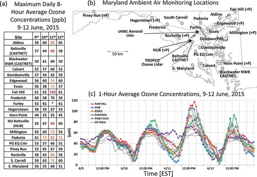
Exceedances of the Environmental Protection Agency (EPA) National Ambient Air Quality Standard (NAAQS) for surface ozone (O₃) have dropped to record low levels in Maryland in 2013, 2014, and 2015 (MDE, 2015c). This was due primarily to regulatory measures such as the NOx State Implementation Plan (SIP) Call of 2002 (Aburn et al., 2015) that lead to regional reductions of anthropogenic NOx (nitrogen oxides), an ozone precursor (Gégo, et al., 2007), and a decline of the annual average number of exceedance days from 52 during 2000–2002 to 7 during 2013–2015 under the 2008 O₃ NAAQS of 75 ppb. Wildfire smoke subsided and dipsersed within the United States (U.S.) Mid-Atlantic (MA) planetary boundary layer (PBL) during this contemporary clean period on June 9–12, 2015. The first 2015 Maryland exceedance of the 75-ppb 2008 O₃ NAAQS occurred on June 11 as O₃ concentrations increased to levels not observed since prior to the record low period. Using the lower 70-ppb 2015 O₃ NAAQS (EPA, 2015), a 3-day O₃ exceedance episode occurred that caused Maryland to miss attainment of the new 70-ppb O₃ design value, the metric with which EPA measures compliance. Subsequent discussion of O₃ focuses on the 2015 70-ppb NAAQS (2008 values are indicated in parentheses for contrast with the most recent regulation values). During the smoke event, 50% (30%) of Maryland sites (Figure 1a) exceeded the 2015 (2008) 70 (75) ppb NAAQS on June 11 as the smoke impacted surface O₃ precursors, sinks, and reservoirs.

Figure 1. (a) Site names and daily 8-hr maximum ozone, (b) monitoring locations throughout Maryland used in the study, and (c) the 1-hr ozone concentrations at each of the sites from June 9–12, 2015. Colored sites are specifically referenced within the text. The 8-hr concentrations exceeding the 2015 NAAQS standard are highlighted by new standard AQI colors in (a). Monitoring locations which also have co-located hourly BAM PM_2.5 monitors are shown with a (+P). Light gray lines are major interstates in Maryland. *No afternoon 8-hr average was available at Furley due to instrumentation errors caused by HVAC issues in the building holding the unit. Furley is also near the Oldtown PM_2.5 BAM monitor in downtown Baltimore. Oldtown does not have ozone measurements.

Wildfires are known sources of both primary and secondary pollutants, including carbon monoxide (CO), fine particles (PM_2.5), NOx, volatile organic compounds (VOCs; Hu et al., 2008), and O₃ (Andreae and Merlet, 2001; McKeen et al., 2002; Bytnerowicz, et al., 2010). Similar to the study presented here, Canadian wildfires have increased O₃ concentrations in Houston, TX (Morris et al., 2006), and as far away as Europe (Spichtinger et al., 2001). Evidence of Canadian wildfire smoke and biomass burning affecting the MA’s particulate matter (PM) air quality was also previously reported (Adam et al., 2004; Colarco et al., 2004; Sapkota et al., 2005), but wildfire smoke has also been recognized in high-O₃ events on the East Coast (Fiore et al., 2014). DeBell et al. (2004) presented a chemical characterization of the July 2002 Quebec wildfire smoke plume and its impact on atmospheric chemistry in the northeastern United States. However, limited and insufficient detailed observational analyses during smoke events have been performed, especially in the U.S. MA under contemporary regional emissions.

Wildfire emissions themselves are harmful to human health, but are exacerbated within urban pollution (Kunzli et al., 2006) and are difficult to quantify (McKeen et al., 2002). Singh et al. (2012) outlined some of the current shortcomings in the Community Multiscale Air Quality (CMAQ) model associated with wildfire smoke. Others have noted the uncertainties in the influence of wildfire emissions on O₃ production (e.g., Hu et al., 2008). Characterizing and accurately modeling wildfire constituents in the MA is important for future air quality forecasts and modeling, particularly for regulatory and compliance issues related to NAAQS exceedances associated with wildfire O₃ production in the United States (Jaffe and Wigder, 2012). While infrequent in the MA, wildfire smoke may be an increasing fractional contribution to high-O₃ days, particularly in light of increased fire frequency in a warming climate (Flannigan and Wagner, 1991; Westerling et al., 2006; Marlon et al., 2009; Spracklen et al., 2009; Pechony and Shindell, 2010), decreasing regional emissions (Gégo, et al., 2007), and tighter O₃ NAAQS (EPA, 2015).

With partnership from academic and federal agencies, the Maryland Department of the Environment (MDE) maintains a dense network of in situ and remote sensing pollution sampling platforms in Maryland (Figure 1b). Surface monitors used for regulatory purposes include 20 O₃ monitors (including two EPA CASTNET sites; EPA, 1997), nine hourly PM_2.5 beta attenuation monitors (BAMs) with additional PM_2.5 hourly observations from locations in Washington, DC (DC), and northern Virginia, various daily PM_2.5 Federal Reference Method (FRM) filter speciations, VOC canisters, extinction monitor, nephelometer, and aethalometer. A full description of the various kinds of instrumentation used by MDE is available in the MDE Network Plan (Maryland Department of the Environment, 2015a). Remote sensing instrumentation includes a 915-MHz radar wind profiler (RWP; Ryan, 2004; MDE, 2015b), Elastic Lidar Facility (ELF) aerosol lidar (Delgado et al., 2015), and NASA Goddard Space Flight Center TROPospheric OZone DIfferential Absorption Lidar (GSFC TROPOZ DIAL, Sullivan et al., 2014). Combined with other regional data from EPA’s Air Quality System (AQS), this network provided a high-resolution observational data set of a rare air quality event in the MA associated with aged Canadian smoke.

Here we first describe the regional smoke event from June 9–12, 2015. Both heightened PM_2.5 and O₃ pollution were noted along the smoke plume trek from Canada to the MA. However, lidar and surface observations show that additional wildfire smoke subsided during transport over the northern MA, causing direct and indirect consequences at the surface. Surface O₃ concentrations in particular showed a rapid response at the height of the event on June 11 (Figure 1c) as smoke constituents increased. Discussion of aerosols, O₃, and O₃ precursors observed during the event follow. These connect remote sensing and surface observations to smoke subsiding into the PBL, and investigate an O₃ lag with respect to smoke onset believed to be related to wildfire-related VOCs and an O₃ decrease behind a Chesapeake Bay Breeze (BB), historically associated with enhanced O₃ northeast of Baltimore, MD (Piety, 2007; Landry, 2011). Additionally, the first collocation of O₃ lidar and RWP is shown within the MA, observing O₃ associated with the nocturnal low-level jet (NLLJ). Lastly, comparison of the National Oceanic and Atmospheric Administration (NOAA) operational CMAQ surface O₃ forecast to regional surface observations provides an estimate of ozone contribution from the smoke.

The smoke event

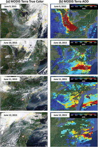
In late May and early June 2015, abnormally warm and dry weather across central Canada was conducive to wildfires. Fires in Saskatchewan were ignited by lightning on June 6, 2015, and consumed approximately 77,000 acres by June 8 (Canadian Interagency Forest Fire Centre [CIFFC], 2016) in areas comprised of spruce, pine, aspen, poplar, and firs (University of Saskatchewan, 2006). Uncontained fires created a prodigious smoke plume with large aerosol optical depth (AOD) detected in satellite retrievals (Remer et al., 2005), as shown in Figure 2. The plume was impacted by a developing mid-latitude cyclone tracking east along the U.S.–Canada border, which pushed a cold front southward through the Great Lakes, Ohio River Valley (ORV), and MA by the evening of June 9, 2015. The resulting wind patterns transported the smoke approximately 3100 km from Canada to the MA in 3 days. Smoke lingered in the MA under the influence of a high-pressure system until removed by southerly winds on June 12, 2015.

Figure 2. (a) Red–green–blue (RGB) “true color” images of Canadian wildfire smoke over the Mid-Atlantic United States from the NASA MODIS Terra sensors and (b) corresponding MODIS Terra Aerosol Optical Depth (AOD) on June 9, 10, 11, and 12, 2015. The star indicates the location of the Howard University-Beltsville (HUB) campus in Maryland. Note that June 11 and 12 images cover a smaller domain. Source: Space Science and Engineering Center, University of Wisconsin-Madison (http://ge.ssec.wisc.edu/modis-today) and Infusing Satellite Data into Environmental Applications (IDEA, http://www.star.nesdis.noaa.gov/smcd/spb/aq/index.php).

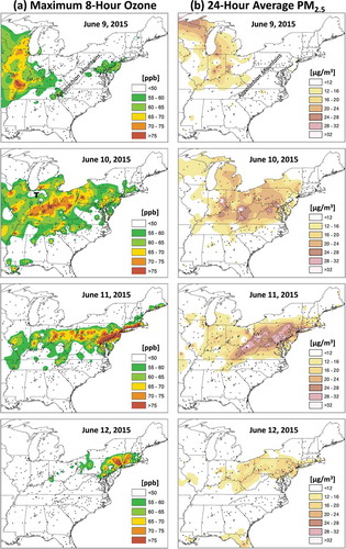
Increased surface PM_2.5 concentrations tracked well with the smoke plume from Canada to the northern MA, but heightened O₃ concentrations and associated 2015 O₃ NAAQS exceedances lagged the increased PM_2.5 (Figure 3). For example, on June 9 PM_2.5 was greater than 12 µg m⁻³ statewide in Indiana, but O₃ was primarily <50 ppb in the state. Instead, the highest maximum 8-hr averages, 60–72 ppb concentrations, were across Illinois and southern Wisconsin. On June 10, PM_2.5 had increased in Maryland but peak O₃ was in Ohio and western Pennsylvania with mid-60s to 80 ppb maximum 8-hr averages. By June 11, O₃ dramatically increased in the MA, with a maximum 8-hr average of 100 ppb in northeast Maryland (Figure 3). Ozone decreased on the afternoon of June 12 as smoke cleared the region.

Figure 3. June 9–12 daily (a) maximum 8-hr average ozone (ppb) and (b) 24-hr average fine particle concentrations (µg m⁻³) across the eastern United States. Ozone and PM_2.5 line up spatially with the smoke plume trek from the upper Midwest to the Mid-Atlantic by June 11. Pollutants were spatially interpolated using a tension spline method. Black dots show the location of monitors of the respective pollutant. The approximate location of the Appalachian Mountains is labeled for reference. “T” denotes an area of Indiana impacted by thunderstorms. Source: EPA’s Air Quality System (AQS).

Meteorology

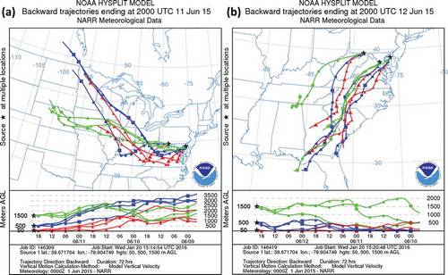
Cyclonic flow around a mid-latitude cyclone tracking along the U.S.–Canada border supported smoke transport from Saskatchewan, Manitoba, and Minnesota beginning on June 8 per NOAA Air Resources Laboratory (ARL) 32-km resolution North American Regional Reanalysis (NARR; Mesinger et al., 2006) Hybrid Single-Particle Lagrangian Integrated Trajectory (HYSPLIT; Rolph, 2015; Stein et al., 2015) 72-hr backward trajectories originating in Maryland at 4:00 p.m. EST (2000 UTC) on June 11 (Figure 4a). Another mid-latitude cyclone moved along the U.S.–Canada border on June 10, stalling another cold front west to east across the middle of Pennsylvania but turning and preserving westerly mid- and low-level tropospheric winds across the ORV through June 11. The secondary cold front accounted for the sharp gradient in O₃ and PM_2.5 across Pennsylvania and little pollution across upper New York State on June 11 (Figure 3). With surface high pressure centered across the eastern ORV on June 10–11, light surface winds in Maryland allowed the smoke to linger.

Figure 4. National Oceanic and Atmospheric Administration (NOAA) Air Resources Laboratory (ARL) Hybrid Single-Particle Lagrangian Integrated Trajectory (HYSPLIT), model vertical velocity, 72-hr backward trajectories using the North American Regional Reanalysis (NARR) data set from a spread of locations in Maryland beginning at 4:00 p.m. EST on (a) June 11, 2015, and (b) June 12, 2015. Stars show the start locations of the trajectories. Trajectory meteorological fields are at 50 m (red triangles), 500 m (blue squares), and 1500 m (green circles) above ground level. Shapes are plotted at 6-hr intervals. Near-surface transport switched to southwesterly on June 11, while higher heights showed west and northwesterly transport consistent with the track of the smoke. All trajectories indicate some degree of subsidence from June 10 to June 11. Trajectories ending at 500 m above sea level subsided from roughly 3 km.

Warm air from the Great Plains (1500 m trajectories, Figure 4a) helped maximum surface temperatures increase to 30–35°C (~86–95°F) in Illinois on June 9, in Ohio on June 10, and in the MA on June 11. Concurrently, the smoke plume crossed the trajectory of the warm air (500 m, Figure 4a) while over the ORV. As the warm air moved in to the MA, initial temperatures at 850 hPa at Sterling, VA (IAD, 39.98° N, 77.49° W) (not shown here; University of Wyoming Department of Atmospheric Science [UW], 2015), which act as a proxy for summer surface temperatures, increased from 13°C at 1200 UTC on June 10 to 19°C by 1200 UTC on June 11. Observations (National Climate Data Center [NCDC], 2015) at Baltimore Washington International Airport (BWI, 39.17° N, 76.67° W), located 22 km northeast of the Howard University Beltsville (HUB) site and ~13 km south of Baltimore, were generally representative of Maryland regional surface conditions. The maximum surface temperature at BWI on June 10 was 28.9 ºC (84ºF), near the normal 27.8ºC (82ºF). Maximum surface temperatures increased on June 11 and 12 to 33.9ºC (93ºF) and 34.4ºC (94ºF), respectively. Surface winds at BWI were initially from the northwest behind the June 9 cold front, but turned south-southwesterly (~200º) on June 10–12, changing the transport regime into Maryland to deep southerly origins (Figure 4b) and moving smoke northward. Daytime (9:00 a.m. to 7:00 p.m) wind speeds, which averaged ~2.6 m s⁻¹ on June 10 and 11 (illustrated with the RWP), averaged 4.2 m s⁻¹ on June 12.

Aerosols

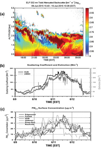
The transport path of smoke-filled air is dependent on the transport altitude (DeBell et al., 2004), so an estimate of the smoke plume height is critical for understanding its transport history. Aerosol lidar observations at the University of Maryland Baltimore County (UMBC) Elastic Lidar Facility (ELF) in Catonsville, MD (39.25° N, 76.70° W), monitored the vertical distribution of aerosols over the Baltimore–Washington, DC, metropolitan region to supplement surface measurements. Detailed description of ELF system specifications and data analysis algorithms have been reported elsewhere (Delgado et al., 2015). Based on aerosol lidar observations (Figure 5a), the smoke plume arrived over the Baltimore region at an altitude of at least 3.5 km above ground level (AGL), then subsided to and became well mixed within the PBL in the early morning hours of June 10 behind the aforementioned cold front. Increases (red counts) in the attenuated backscatter time series act as a proxy for smoke within the PBL. Correlation between PM_2.5, particle scattering, and extinction measurements made at HUB and UMBC, respectively, was also observed, as shown in Figure 5b. Surface scattering and extinction measurements at HUB and UMBC were obtained with an Ecotech Aurora 1000 nephelometer (525 nm) and an Aerodyne CAPS PMex Extinction monitor (532 nm), respectively. The high values reported by these two optical monitors corroborate the lidar observations, showing smoke subsidence to the surface. Surface extinction rose sharply on the evening of June 10 and persisted into June 11. The near-surface lidar attenuated backscatter increases and extinction measurements coincided with a regional increase in the hourly PM_2.5 concentrations, nearly doubling, from 5–10 µg m⁻³ in the evening of June 9 to approximately 15–20 µg m⁻³ in the early morning hours (beginning near 7:00 a.m. EST) on June 10 (Figure 5c). PM_2.5 concentrations greater than 30µg m⁻³ were observed in Maryland during this smoke episode, as more smoke mixed into the PBL. The highest daily average PM_2.5 at Maryland BAMs over the 4-day event was 32.5 µg m⁻³ at the HUB air quality monitoring station on June 11, not exceeding the 2012 PM_2.5 24-hr average 35.4 µg m⁻³ NAAQS.

Figure 5. (a) UMBC ELF aerosol lidar time series from June 9, 2015, at 3:40pm (15:40) EST to June 10, 2015 at 10:28 a.m. EST. (b) Scattering coefficient and extinction over the course of the event, including corresponding times in (a) at HUB and UMBC, respectively. (c) Hourly averaged fine particle (PM_2.5) concentrations for all Maryland monitoring sites showing the subsiding signature captured by the ELF in (a) was associated with rising particle counts.

Ultraviolet radiation

Wildfire particle pollution alters the radiative flux at the surface by scattering and absorbing solar radiation (Penner et al., 1992), with consequences to atmospheric stability and secondary pollutant production (Taubman et al., 2004; Hodzic, et al., 2007). Smoke in the present case attenuated incoming ultraviolet (UV) light. Cloud and smokeless sky conditions on June 9 (pre event) yielded maximal UV radiation of 54.3 W m⁻² from 1-minute average observations. Minute data were first smoothed with a 10-min moving average. The UV measurements (295–385 nm) were taken with a EPLAB Total Ultraviolet Radiometer (The Eppley Lab, 2015) at the MDE Essex air quality monitoring site 21 km east of the UMBC aerosol lidar and are considered reference UV flux in the absence of smoke (Table 1). On June 10 and 11, the maximum measurements were 46.7 W m⁻² and 49.0 W m⁻², respectively, indicating a 14.0% and 9.8% decrease in UV flux in the lower atmosphere. Given the thick nature of the smoke plume on June 10 (Figure 2b), this UV reduction/attenuation was due to the smoke (Taubman et al. 2004). By June 11, 2015, the highest AOD was off the MA coast over the Atlantic, as shown in Figure 2c, which allowed a moderate increase of UV flux to the surface layer in Maryland with respect to June 10.

Table 1. Maximum ultraviolet (UV) radiation from the radiometer at Essex, MD, from June 9–12.

	Maximum UV radiation (W m-2)	Percent reduction from June 9
June 9	54.3	—
June 10	46.7	14.0%
June 11	49.0	9.8%
June 12	53.1	2.2%

Note. A 10-min moving average was applied to smooth minute average data. Smoke decreased UV intensity during the smoke event, given as a percent decrease as compared to a cloud- and smoke-free June 9.

Potassium and organic carbon smoke markers

Particle pollution generated from biomass burning is typically dominated by organic carbon (OC) and black carbon (BC; Martins et al., 1998), and possesses ions such as potassium (Lee et al., 2010). Ionic potassium (K⁺) acts as a useful tracer of wildfire smoke because there are few anthropogenic sources, and concentrations above background levels are a signature of wildfire emissions. Concentrations of K⁺ and OC were amplified across the northern MA (Figure 6). Daily average concentrations of K⁺ on June 11 from MDE’s Chemical Speciation Network monitors at Essex and HUB were 0.153 and 0.171 µg m⁻³, respectively. Compared to averages of 0.037 µg m⁻³ and 0.046 µg m⁻³, respectively, for all nonsmoke days in the month of June, the June 11 measurements indicated a fourfold increase. Similar K⁺ concentrations were reported from West Virginia to southeastern Pennsylvania (Figure 6a).

Figure 6. (a) Potassium ion (K⁺) and (b) organic carbon (OC) spatially interpolated daily concentration (µg m⁻³) surface observations on June 11, 2015. Pollutants were spatially interpolated using a tension spline method. The greatest concentrations of these wildfire attributable pollutants stretched from West Virginia northeastward towards southeastern Pennsylvania. The brown star shows the approximate location of Shenandoah National Park as referenced in the text. Black dots show the location of monitors of the respective pollutant. Source: EPA’s Air Quality System (AQS).

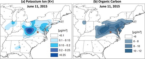
PM_2.5 filter-based 24-hr average OC measurements collected on June 11 from around the region showed a pattern similar to K⁺ observations (Figure 6b). Concentrations ranged from 6.44 µg m⁻³ in Henrico, County, Virginia (Richmond, VA), to ~11.0 µg m⁻³ in the Washington, DC–Baltimore to southeastern Pennsylvania corridor. These values represent a factor of three increase in Richmond, and a fivefold increase in Maryland and southeast Pennsylvania compared to the range of all other nonsmoke sample averages collected in June 2015 (1.8–2.5 µg m⁻³).

Based on K⁺ and OC observations, the greatest surface smoke concentrations on June 11 were centered from West Virginia north of a line running from Shenandoah National Park, Virginia, to DC, Philadelphia, and to New Jersey (Figure 6). K⁺ and OC observations suggest more than double the surface smoke concentrations in locations such as northern Maryland and southeast Pennsylvania compared to elsewhere. A corridor of heightened PM_2.5 and O₃ formed in these same areas on June 11 (compare Figures 3 and 6), implying a role of smoke in the development of these features. This also implies that heightened O₃ concentrations in places like Connecticut on June 11 may not have been associated with smoke as they were in the northern MA.

Aethalometer and black carbon

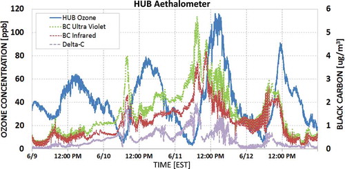
An aethalometer located at the HUB site indicated heightened black carbon (BC) during the event (Figure 7). While BC is also sourced from mobile emissions, globally one-third of BC is sourced from biomass burning (Lamarque et al., 2010; U.S. EPA, 2010). The optical absorptions of UV (370 nm) and near-infrared (880 nm) wavelengths of the aethalometer are generally very similar when observing anthropogenic-sourced particles such as diesel exhaust, but increased absorption at shorter wavelengths causes a separation of the signals (deemed “Delta-C”) while observing naturally sourced BC (Hansen, 2005; Allen et al., 2004). Beginning on the evening of June 9 and coincident with the first arrival of smoke at the surface observed by the UMBC aerosol lidar (Figure 5a), the two aethalometer signals separated, with more power from the UV wavelengths, implying the increased Delta-C was due to wildfire BC particles (Hansen, 2005). The actual magnitude of BC was represented by the 880-nm (near-infrared) signal and indicated a rise from a baseline of ~0.5 to 4.0 µg m⁻³ by June 11. Given the preponderance of evidence of smoke and the coincidental timing of the Delta-C increase, Delta-C and BC can also be considered tracers of wildfire smoke near the surface. Under this assumption, June 11 exhibited the greatest concentrations of surface smoke. The greatest O₃ concentrations over the 4-day period also occurred on June 11. This was a noteworthy coincidence to the lag in O₃ between June 10 and 11 and the increase in surface extinction later on June 10, compared to the smoke arrival late on June 9 in Figure 5.

Figure 7. Minute averaged ozone concentrations at HUB site, (blue), infrared (880 nm, red) and ultraviolet (370 nm, green) channels, and Delta-C (purple) black carbon concentrations (µg m⁻³) observed by the HUB aethalometer. The UV and red channels separate late in the day on June 9 with a greater UV signal return, suggesting an increase in naturally sourced black carbon concentration and an indicator of smoke. The two channels generally remain apart through midday on June 12.

Ozone exceedance

Despite smoke in Maryland on June 10 (Figures 2 and 3), widespread exceedances of the O₃ NAAQS thresholds (2008 and 2015) in Maryland did not occur until June 11, 2015 (Figure 1a). The 1-hr O₃ concentrations (Figure 1c) for the MDE sites (Figure 1b) illustrated the disparity in O₃ magnitudes between June 10 and 11. Only one site in Maryland climbed above 70 ppb on June 10, but 10 sites increased to more than 70 ppb on June 11. This was partially explainable due to the temperature increase. Though it was relatively warm on June 10, a greater probability of O₃ NAAQS exceedance in Maryland exists with higher temperatures (Lin et al., 2001), and historically, MDE has tracked Maryland’s O₃ exceedance days with temperatures equal to or exceeding 32.2ºC (90ºF) (MDE, 2012; Warren, 2013).

At an elevation of approximately 768 m above sea level (ASL), night observations at the Piney Run monitor are considered a sample of the nocturnal residual layer by MDE and a measure of transported pollutants. Between June 10 and 11, 2015 (Figure 1b), O₃ concentrations near 60 ppb persisted through the night (Figure 1c), indicating an elevated O₃ “reservoir” crossing the mountains from the ORV, consistent with Figure 4a trajectories. Concurrent with the pollution transport, air at 850 hPa measured over IAD characterized by 19ºC temperatures and that previously mixed with the smoke plume (Figure 4) advected into the MA on the evening of June 10, increasing maximum surface temperatures on June 11. These more O₃-conducive conditions created Red/Unhealthy air quality index (AQI) conditions (8-hr average O₃ greater than 85 (95) ppb) in Maryland, the first verification of Unhealthy AQI since 2012. Orange/Unhealthy for Sensitive Groups (USG) AQI (8-hr average O₃ greater than 70 (75) ppb) was focused along and north of Interstate 95 (I-95) in Maryland, but elevated Yellow/Moderate AQI (8-hr average O₃ greater than 54 (59) ppb) was regionally observed, particularly north of DC along the Maryland–Pennsylvania state line. As noted in the earlier aerosol discussion, this region had the highest concentrations of particle pollution and aerosol smoke tracers (PM_2.5, OC, and K⁺). Hourly O₃ concentrations above 100 ppb were reported in two locations, HUB and Fairhill (Figure 1c), with the latter reaching a maximum of 118 ppb and remaining above 100 ppb for 5 hours. In total, there were 10 (6) Maryland sites or 50% (30%) of the network that exceeded the 2015 (2008) 8-hr O₃ NAAQS on June 11, 2015.

The magnitude of smoke sourced BC (per Delta-C on Figure 7; Allen et al., 2004) rose again on the morning of June 12, coincident with another steep rise in O₃. However, after 9:00 a.m. EST, the Delta-C dropped under 0.5 µg m⁻³ and by 11:00 a.m. the total BC present dropped to June 9 pre-smoke-event levels. Despite full sun and temperatures greater than 32.3°C (90°F), minute-averaged O₃ concentrations dropped below 50 ppb from peak minute averages of 90 ppb at 11:30 a.m. Southerly wind speeds increased, the trajectory regime changed (Figure 4b), and smoke was transported and dispersed northward downwind of Maryland. Hourly O₃ concentrations dropped from south to north from late morning through early afternoon (Figures 1c and 7). The highest 8-hr average of the day (Padonia, 71 ppb) exceeded (fell short of) the 2015 (2008) O₃ NAAQS. All other state monitors observed 65 ppb or less for their maximum 8-hr average. Despite initially O₃ conducive conditions on June 12, no sustained O₃ production occurred as winds removed smoke from the local environment.

Continuous ozone lidar observations

Partnership between the UMBC, NASA, and MDE made available the NASA Goddard Space Flight Center TROPospheric OZone DIfferential Absorption Lidar (GSFC TROPOZ DIAL; Sullivan et al., 2014), which was developed and validated within the Tropospheric Ozone Lidar Network (TOLNet). The TROPOZ system has accurately resolved O₃ concentrations to within 10% of nearby ozonesonde launches and simulated profiles (Sullivan et al., 2015a, 2015b). During the smoke event the O₃ lidar was located at HUB and captured nearly continuous vertical profiles of O₃ from 10:00 a.m. on June 11, 2015, to 5:00 a.m. on June 12, 2015 (Figure 8a), providing spatiotemporal resolution of O₃ not before available for the MA region. During the morning hours of June 11 the lidar resolved an O₃ reservoir of 60 ppb or greater within the residual layer between 1000 and 1500 m. This was a similar portion of the residual layer where Piney Run (elevation of approximately 768m) sampled nearly 60 ppb of O₃ through the morning of June 11 (Figure 1c). The lidar observed rapid O₃ production during the late morning hours on June 11, and eventually, concentrations between 90 and 120 ppb of O₃ were measured throughout the depth of the boundary layer. Superimposed on the O₃ lidar image was an ozonesonde (triangle, Figure 8a) also launched from HUB at 2:51 p.m. that observed O₃ concentrations in the boundary layer in excess of 120 ppb with considerable agreement to the lidar, attesting to the robustness of the lidar retrieval.

Figure 8. (a) Ozone time series from the GSFC TROPOZ DIAL. The triangle indicates an ozonesonde launch. The bottom color bar shows the surface concentrations. White areas are due to noise or clouds that have no data available. (b) Winds as observed by the MDE HUB radar wind profiler at the same time as in (a). Winds are given in m s⁻¹. Contours are every 2 m s⁻¹. The green area shows the low-level jet.

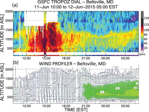
O₃ measured at the lidar site (Figure 8a, color strip, bottom of image) and through the boundary layer decreased after 5:00 p.m. (17:00) EST and continued a downward trend through the night. Nevertheless, the lidar observed an O₃-rich residual layer with 60–80 ppb O₃ through the overnight hours (Figure 8a, approximately 600–1400 m from 8:00 p.m. to 5:00 a.m. EST [20:00–05:00 in figure]). The MDE RWP located at HUB observed a nocturnal low-level jet (NLLJ) beginning around 9:00 p.m. (21:00) EST from the southwest peaking between 500 and 1000 m ASL with winds greater than 12 m s⁻¹. Comparison of the O₃ lidar to the RWP showed the largest residual layer O₃ concentrations occurred immediately above the NLLJ maximum wind speed. It is believed this is the first co-locating of these types of observations in the MA, allowing a never-before-seen correlation of the NLLJ and O₃, substantiating earlier claims that the NLLJ can be linked to pollution transport in Maryland (Ryan, 2004). O₃ concentrations increased with time within the residual layer immediately above the NLLJ wind peak, particularly around 3:00 a.m. on June 12. However, at the same time O₃ above 1500 m and also below 1000 m decreased below 20 and 70 ppb, respectively, per the lidar observations. Given the south-to-north smoke gradient (see Figure 6), it seemed the NLLJ overall acted to remove smoke from Maryland. As previously mentioned, southerly winds on June 12 were responsible for “cleanout.” Further work is planned to discern the full role of the NLLJ in this case.

Carbon monoxide

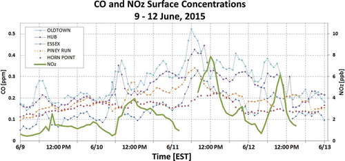
Carbon monoxide (CO) has been previously identified as a wildfire smoke indicator (Andreae and Merlet, 2001; McKeen et al., 2002, DeBell et al., 2004), can play a role in O₃ production, and followed similar trends to other pollutants over the 4-day event (Figure 9). Highest concentrations of CO in Maryland were in northerly locations, in spatial agreement with the previously defined smoke area. For instance, comparison of Piney Run, Oldtown, and HUB to Essex and Horn Point show that the latter two monitors, which are more south and east than the other three in the group (Figure 1b), generally had lower CO concentrations through the period. Statewide-averaged observations showed an increase in CO concentrations from a daily average of 0.17 to 0.30 part per million (ppm) from June 9 to 11. The highest 1-hr average concentrations exceeded 0.50 ppm at the Oldtown monitor in Baltimore City, roughly a doubling of CO content above presmoke concentrations. This is lower than the 0.525–1.025 ppm CO enhancements observed during the Quebec fires of 2002 (DeBell et al., 2004), but by comparison those measurements only traveled approximately 1–2 days and 1000 km from the smoke source and were in a noncontemporary (greater) regional emissions environment.

Figure 9. Hourly carbon monoxide (CO) for all available Maryland monitors and hourly NOz from the Beltsville CASTNet site for June 9–12, 2015. The increased NOz, particularly around midday of June 10–12, suggests long-range transport of NOx species. Data was unavailable from 3:00 a.m. until 8:00 a.m. on June 11 and again after 3:00 p.m. on June 12.

Volatile organic compounds

Hu et al. (2008) emphasized the importance of VOC concentrations from biomass smoke on O₃ production in a winter O₃ event, showing that O₃ production was more dependent on VOCs than on NOx, the two primary precursors to ozone. In the June 2015 case there was evidence of VOCs tracking with the smoke plume. Daily total nonmethane organic compounds (NMOC) observations are spatially sparse. However, daily averaged chromatograph observations retrieved from AQS in Gary and Indianapolis, IN, showed 27% and 118% (23.3 ppbc and 61.0 ppbc) increases in total NMOC, respectively, on June 9 when Indiana was first impacted by smoke (Figure 3b), compared to an average of June 8 and 10 concentrations (pre and post smoke) in those locations. In Maryland, the daily total NMOC concentrations rose by 70% between June 9 and 11 from 40.4 ppbc to 68.7 ppbc as smoke settled over the area, suggesting VOCs tracking with the smoke plume.

Total VOC concentrations also increased between June 10 and 11 in Maryland. Specifically, VOC concentrations during “O₃ production hours” or when strong sunlight and a mixed PBL exist, between 9 a.m. and 7 p.m. local time, increased by 50% from roughly 40 ppbc to 60 ppbc in total NMOC between the two days at the Essex, Maryland, Photochemical Assessment Monitoring Station (PAMS) hourly chromatograph (Table 2). A similar increase was noted in target hydrocarbon (Target PAMS) species. Thus, the majority of the VOC increase occurred between June 10 and 11, well after the first smoke constituents arrived in Maryland.

Table 2. Speciated volatile organic compound (VOC) concentrations from hourly chromatograph data at Essex.

Name	June 9	June 10	June 11	June 12	Percent change
TNMOC	38.10	39.83	59.80	50.00	56.95
Target PAMS	34.70	36.10	54.32	44.90	56.54
Isoprene	1.91	1.89	3.94	3.99	106.28
Ethene	0.92	1.36	1.78	1.40	93.48
Ethane	8.93	7.24	8.34	4.80	−6.61
Benzene	0.62	0.75	1.16	0.67	87.09
Propene	0.66	0.74	0.89	0.77	34.85
Toluene	1.49	1.67	2.50	2.50	67.78
Xylenes	0.42	0.49	0.84	0.74	100.00
Acetone	—	—	—	—	—

Note. Concentrations given are the average during ozone production hours (9:00 a.m. to 7:00 p.m.). The higher resolution of the hourly chromatograph compared to canister data shows a VOC rise from June 9 to the peak of the smoke event on June 11. The percentage change shows the increase of June 11 over presmoke conditions on June 9.

Simpson et al. (2011) studied emissions of nonmethane VOCs (NMVOC) from fresh Canadian wildfire plumes and found that a very small number of NMVOCs represented a large fraction of the total mass of VOCs within the smoke. Some of the chief species were formaldehyde, ethene, pinenes, ethane, benzene, propene, and acetone. Though not within the top 10 numerous species in Simpson et al. (2011), toluene, xylenes, and isoprene were also observed and have been reported elsewhere (Hu et al., 2008). On June 11, all but formaldehyde and pinenes were available in Maryland. Chromatograph data showed many of these smoke-attributable VOCs increased compared to presmoke conditions (Table 2). Isoprene, ethene, benzene, and the xylenes in particular doubled in concentration between June 9 and 11.

Canisters sampling 24 hours at a 6-day frequency at Essex and HUB also showed ~40–68% increase in total PAMS and/or NMOC on June 11 (Table 3). Individual VOC species attributable to wildfire smoke showed similar increases. Of seven examined VOC species associated with wildfire smoke (excluding isoprene), all but propene showed ~30–143% concentration increases (Table 3) on June 11 compared to adjacent collection days and all have maximum incremental reactivity (Carter et al., 1995; Carter, 2009) greater than most other VOC species typically observed during Maryland O₃ exceedance days.

Table 3. 24-hour canister collection at Howard U. Beltsville (HUB), Essex (ESX), and Oldtown (OLD).

Compound	Site	Method	June 5	June 11	June 17	Percent change	3-Hr Avg. maximum
Total NMOC	HUB	126	102.49	134.99	89.69	40.48	206.94 (12 a.m.)
	ESX	126	72.25	151.98	108.8	67.89	—
	OLD	—	—	—	—	—	—
Target PAMs	HUB	126	49.72	76.94	43.19	65.62	100.7 (6 a.m.)
	ESX	126	47.16	82.36	63.34	49.07	—
	OLD	—	—	—	—	—	—
Isoprene	HUB	126	3.44	17.01	7.75	204.02	32.68 (3 p.m.)
	ESX	126	0.76	2.72	1.75	116.73	—
	OLD	—	—	—	—	—	—
Ethene	HUB	126	1.34	2.04	0.99	75.11	1.25 (3 a.m.)
	ESX	126	1.09	1.51	1.22	30.74	—
	OLD	—	—	—	—	—	—
Ethane	HUB	126	6.32	9.59	5.68	59.83	13.60 (6 a.m.)
	ESX	126	7.23	12.89	8.33	65.68	—
	OLD	—	—	—	—	—	—
Benzene	HUB	150	0.78	1.44	0.66	100.00	4.28 (6 a.m.)
	ESX	150	0.84	1.68	1.44	47.37	—
	OLD	150	1.26	1.74	0.84	65.71	—
Propene	HUB	126	0.74	0.63	0.38	12.50	1.06 (6 a.m.)
	ESX	126	0.82	0.85	0.60	19.72	—
	OLD	—	—	—	—	—	—
Toluene	HUB	126	2.69	3.81	1.77	70.85	5.95 (6 a.m.)
	ESX	126	2.72	4.92	2.75	79.89	—
	OLD	150	1.19	2.45	1.40	89.19	—
Xylenes	HUB	126	1.90	2.53	1.11	68.11	3.88 (6 a.m.)
(m,p,o)	ESX	126	2.54	3.61	2.04	57.64	—
	OLD	150	1.04	1.12	0.72	27.27	—
Acetone	HUB	150	5.85	13.35	8.37	87.76	—
	ESX	150	6.84	18.06	8.01	143.23	—
	OLD	150	6.69	15.15	9.84	83.30	—

Note. 24-hour canisters sample for a 24-hr period and report an average concentration once every 6 days. Not all VOCs are detected at all sites (dashes). The method column lists the AQS method code used for the VOC sample. All values are parts per billion carbon (ppbc). The percentages listed are the percent change in concentration on June 11, compared to the average of June 5 and June 17 concentrations. The maximum concentration of the eight 3-hr canisters collected on June 11 at HUB is reported with the corresponding start of the 3-hr collection in parentheses.

The combined increase of all wildfire-attributable species was larger than that of isoprene. Isoprene has been identified as a leading VOC in Maryland O₃ production (Halliday et al., 2015) and is primarily related to biosphere releases due to atmospheric heat stress (Seinfeld and Pandis, 1998) but can also be caused by heat from fires (Simpson et al., 2011; Lee et al., 2008). Isoprene showed a significant increase on June 11 compared to adjacent days and other VOC species during ozone production hours (Table 2) and within a 24-hr canister sample (Table 3). Other canisters sampling a 3-hr period every 3 hr on June 11 at HUB similarly detected a large increase in isoprene from 5.5 ppbc to 32.7 ppbc (Table 3) between 6:00 a.m. and 3:00 p.m., likely due to the quick temperature increase on June 11. In fact, much of the total Target PAMS VOC 24-hr canister increase (refer to Table 3) is attributed to isoprene; it was 7% of Target PAMS on June 5 but 22% on June 11 at HUB. Overall the isoprene increase was greater than any other individual wildfire-related VOC increase. Both the HUB 3-hr canister and the Essex chromatograph showed similar percentage increases in isoprene during the afternoon of June 11 over June 10; however, isoprene was similar on June 11 and 12 at Essex with significantly lower O₃ observed there on June 12, implying isoprene did not singly drive O₃ production. Isoprene made up 22% of Target PAMS VOCs at HUB, but collectively ethene, ethane, benzene, propene, toluene, the xylenes, and acetone made up 43.5 and 52.8% of the total PAMs species on June 11 at HUB and Essex, respectively, suggesting organic VOCs associated with smoke played a key role in ozone production.

Nitrogen oxides

Increased NOy (sum of all oxides of nitrogen) was observed during the event. Singh et al. (2012) showed that O₃ production rates from wildfires in California were dependent upon available NOx (NOx = sum of nitrogen oxide (NO) and nitrogen dioxide (NO₂)) and that NOx from the fires themselves was relatively low. While some NOx may have originated at the fire source, regional anthropogenic NOx emissions undoubtedly played some role in generating high O₃ concentrations as urban pollution mixed with the smoke. Hourly averaged NOz (NOy – (NO₂ + NO)) at the Beltsville CASTNet site (~6 km southeast of HUB) was greater than any other observations taken during the month. NOz represents all non-NOx oxidants of nitrogen and includes NOx reservoir species such as peroxyacetyl nitrate (PAN), which can release O₃-relevant NOx at later times and locations (Jacob, 1999, chap. 11). There are known problems with NO₂ measurements and by extension NOy and NOz (Dunlea et al., 2007); however, the large magnitude of NOz during the smoke period compared to the rest of the month makes these difficulties insignificant to the simple conclusion that more reservoir species were present on June 11 than any other time of the month. On June 11, daily averaged NOz was 1.5 ppb (39%) higher than the second highest day in June (2.32 ppb, June 25), exclusive of other smoke event days (June 10, 12).

Regardless of the NOz and NOx source attribution, wildfire VOCs within the plume can store NOx. PAN for example, is a NOx reservoir species formed by the reaction of NOx and VOCs in the presence of sunlight (Jacob, 1999). Under warm conditions, PAN can be thermally decomposed back into a VOC and an NO₂ molecule, two necessary precursors for ozone, at locations downwind of their source. Thus, the VOC content of the smoke plume could not only impact local ozone production but regulate the quantity of NOx “stored” within the smoke plume. Smoke was transported through the energy-production-heavy ORV on June 10. NOx data extracted from the Clean Air Markets Database showed increased electrical generating unit (EGU) emissions affecting Maryland on June 11 due to rising regional temperatures. In the airshed defined by NARR HYSPLIT 2000 UTC 24-hr backward trajectories at and below 1500 m (see first 24 hr of Figure 4a), total NOx emitted was 493, 550, 612, and 633 tons on June 9, 10, 11, and 12, respectively, increasing 28% compared to the June 9 amounts. Daily emissions across this same area did not vary more than 13% from June 12 to 20, making EGU emissions on these days comparable to the June 12 peak. However, the entire northeast quadrant of the United States experienced no other O₃ exceedances during the remainder of June despite persistent peak emissions. This implies the emission rates from the ORV were not supportive of O₃ exceedances except in the presence of smoke. The 24-hr average NOz concentration on June 11 (3.8 ppb) was three times the average concentration of all other June nonsmoke days of similar EGU emissions (1.31 ppb, June 13–20), and was also greater than two standard deviations above the entire monthly average. Additionally, no other single hour in the month of June surpassed the NOz observed at noon on June 11 (Figure 9). The additional storage within the plume made NOx from any upstream source the smoke crossed potentially available later in the MA.

Influence of the bay

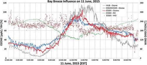
In summertime, the Chesapeake Bay frequently develops breezes due to the unequal heating between the land and water. Historically these breezes have been blamed for enhanced O₃ observed just northeast of Baltimore (Piety, 2007), particularly at the Edgewood, MD, monitor (Landry, 2011; Loughner et al., 2014). A characteristic bay breeze (BB) on-shore wind shift (west-southwesterly to southerly direction) with a coincident rise in relative humidity typical of the bay’s marine air developed after 1:00p.m. EST on June 11, 2015 (Figure 10) and impacted the Essex and Edgewood, MD, monitors. Despite the historical connection between poor air quality and BBs in this area, no exceedance of the O₃ NAAQS occurred at these two monitors. It is hypothesized that southerly winds over the bay on June 11, while light, allowed cleaner (lower smoke concentrations), near-surface air from the south to advect farther north than in other areas of the state. As bay air moved on-shore over Edgewood and Essex, the air was cleaner than at the HUB site, which was farther from the bay and still within the smoke and urban plume. The BB decreased O₃ by 10–20 ppb at Essex and Edgewood around 1:30 p.m. (Figure 10), coincident with a 5-µg m⁻³ decrease in hourly averaged fine particle concentrations at Edgewood (Figure 5c), preventing the two bay-side monitors from exceeding the 75 ppb O₃ standard.

Figure 10. Minute averaged ozone and wind direction at HUB and Essex, MD. Also included is the bayside monitor Edgewood, which is 19 km northeast of Essex. Soon after the characteristic southerly wind shift associated with the Bay Breeze, ozone concentrations dropped 10–20 ppb at both Essex and Edgewood compared to the sustained ozone concentrations observed at HUB.

To further investigate the influence of the bay, O₃ precursors were examined. Average NOx during O₃ production hours was greater on June 11 (11.7 ppb) than on June 10 (7.0 ppb) at Essex, but NOx minute data at Essex showed no appreciable change associated with the BB. There was also more NOx available at Essex (11.7 ppb) than HUB (7.6 ppb) on June 11 during O₃ production hours. Thus, NOx does not singly appear to explain the disparity between Essex and HUB. The concentration of CO at HUB was greater than Essex through the event, however. The O₃ production hours’ average on June 11 at HUB was 0.331 ppm, while it was only 0.238 ppm at Essex. CO at Essex also came in line with the lower Horn Point readings around the time of the BB (Figure 9), suggesting a correlation between CO and the O₃ drop there. The connection of O₃ to CO is further supported by the sharp drop in CO at HUB on June 12 beginning after 10:00 a.m. (Figure 9), coincident with the sharp O₃ and BC decrease seen in the aethalometer (Figure 7), suggesting that the removal of smoke from the ambient air hindered O₃ production. The CO to O₃ mechanism is relatively slow (Jacob, 1999), so the CO may be acting only as a smoke tracer at these short time scales.

The 56% increase in NMOC and Target PAMS VOCs on June 11 over June 10 at Essex during O₃ production hours (Table 2) was likely a conservative estimation of total VOC increase for the Maryland I-95 region between the two days, since Essex also showed a “cleanout” of other species from the BB on June 11. Therefore, it is hypothesized that other monitors, which saw some of the more extreme O₃ concentrations, such as HUB and Fairhill, may have had VOC concentrations far exceeding the 56% increase observed at Essex. What was also striking about the BB passage was that nearly all the coincidental increase of isoprene was behind the BB, in the same air mass that created the O₃ decrease (Figure 10), though overall, isoprene represented a small relative and absolute portion of total NMOCs at Essex.

CMAQ underestimation of ozone

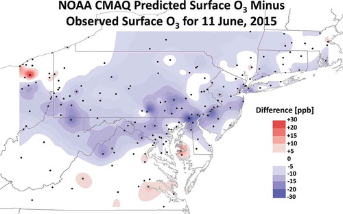
The presence of smoke during the O₃ exceedance provided circumstantial evidence that a significant portion of O₃ production was attributable to smoke. To quantify the attribution, maximum 8-hr average O₃ values forecast with the operational NOAA CMAQ O₃ model were compared to observed concentrations. Source information from the Canadian fires as well as gas-phase chemical interactions from wildfire smoke and their interactions with O₃ was not included in the NOAA operational CMAQ model during 2015. Therefore, the NOAA operational CMAQ model represented a prediction of O₃ in the absence of smoke. With this information, the difference between model forecast and observations on June 11 provided an estimate of the increase in O₃ due to smoke.

Gridded CMAQ data were extracted at observation points throughout the northern MA for June 11. The differences between the predicted and observed 8-hr maximums were interpolated across the MA region and showed an axis of underprediction stretching from northern Virginia through southeastern Pennsylvania (Figure 11). The average difference between the modeled and observed maximum 8-hr average ozone concentration at Maryland monitors north of DC (Hagerstown, Frederick, South Carroll, Rockville, HUB, Beltsville, Furley, Padonia, Aldino, and Fairhill) on June 11 was 14 ppb, with a range of 7.6 to 30 ppb. Similar differences were noted in southeastern Pennsylvania. Note that the geographic distribution of these differences is consistent with surface smoke observations (Figure 6) and PM_2.5 observations on June 11 (Figure 3). The underprediction is also significant since the NOAA CMAQ O₃ model previously reported ~7 ppb high bias and 15.1 ppbv RMSE for June O₃ predictions in the Northeast in 2010 (Chai et al., 2013).

Figure 11. Interpolated differences between point observations and gridded forecasts of the maximum 8-hr average ozone from the NOAA CMAQ operational model (CMAQ predicted ozone minus the ozone observations) in parts per billion (ppb) for June 11, 2015. The analyses domain is confined to an area centered on Maryland. The forecast grid containing the monitor was used for the model to observation comparison. Black dots are ozone monitor locations. Only differences >5 ppb between the model and observations are contoured. Blue shading indicates negative values or underprediction by at least 5 ppb. Red shading indicates positive values or overprediction by at least 5 ppb.

Discussion

The EPA designates an area’s attainment and compliance of the NAAQS via the design value metric. For ozone, the monitor with the greatest annual fourth-highest daily 8-hr maximum concentration averaged over the past 3 years designates attainment status for the region. As of this writing, design values at Padonia and Edgewood are 71 ppb due to O₃ concentrations on June 11 that were the first and second highest ranked observations of 2015 at these monitors, respectively. Excluding the 8-hr maximums on June 11 would lower these design values to 70 ppb and bring the Baltimore Non-Attainment Area (NAA) into compliance of EPA 2015 70 ppb standard. The EPA has granted exception requests for O₃ exceedances due to wildfires in the past (e.g., the 2002 Quebec Wildfires). However, in this study an exception would need to be granted for the Edgewood monitor that did not exceed the 75 ppb O₃ NAAQS. Maryland is therefore burdened with showing that smoke contributed “enough” to the 8-hr average to cause a higher design value. However, it is difficult to quantify wildfire impacts on O₃ concentrations, particularly when mixed with urban pollution (Sing et al., 2012). This highlights the difficulties of such events and the impact wildfire events have on policy. Though wildfires are not new, the issues concerning wildfires and attainment in Maryland are due to lower regional NOx and the tighter standard. Given the policy implications of MA transported smoke on air quality events, accurately modeling and quantifying the effects of these potentially increasing events is of vital importance.

Previous literature has shown that biomass burning can influence downwind O₃ precursor concentrations and therefore O₃ production via increased VOCs, nitrogen compounds and/or CO (Andreae and Merlet, 2001; McKeen et al., 2002; DeBell et al., 2004; Hu et al., 2008; Monks et al., 2009). In the June 9–12, 2015 event, however, a lag existed between enhanced PM_2.5 and O₃ concentrations along the smoke plume trek (Figure 3). In Maryland, smoke arrived a day earlier than when the greatest O₃ concentrations were observed. The most likely explanation was the warmer air that moved eastward from the Great Plains from June 9 to 11 in concert with the O₃ rises, suggesting warmer temperatures were necessary for the O₃ production. This was true in Maryland as the maximum surface temperature increased 5°C between June 10 and 11 at BWI. Rising surface temperatures are positively correlated with EGU NOx production, and thus the warmer temperature can also act as a proxy for additional NOx within the smoke plume that was observed on June 11. The smoke plume was also optically thick (Figures 2 and 5b) and caused a 14% decrease in UV penetration to the surface in Maryland (Table 1). With similar screening under the plume elsewhere, O₃ production and not PM_2.5 pollutants would have been initially affected.

O₃ precursors were in greater numbers on June 11. For example, hourly data from the chromatograph at Essex, MD (Table 2), showed that total NMOCs during O₃ production hours (9:00 a.m.–7:00 p.m.) peaked on June 11, 21.7 ppbc (56.9%) greater than presmoke conditions on June 9, consistent with 40–68% increases in 24-hr canister NMOCs and target PAMs concentrations at HUB and Essex. CO doubled from presmoke concentrations, and long-range transport species of nitrogen oxides (NOz) saw nearly an eightfold increase above presmoke conditions at the peak 1-hr concentration on June 11. These trends matched well with smoke-related observations in PM_2.5 and aethalometer data, all strongly implying their increases were associated with the smoke plume. Comparison of PM_2.5 on June 10 and 11 also suggest possible secondary organic aerosol (SOA) formation. Smoke first arrived between June 9 and 10, yet concentrations were still ~8–10 µg m⁻³ higher on June 11 region-wide with a particularly focused southwest to northeast axis across northern Maryland (Figures 3, 6a, and 6b). SOA formation is hypothesized as the cause for this heightened corridor of PM_2.5. This again was the same corridor where the CMAQ model underpredicted ozone formation by around 14 ppb in Maryland, implying a direct connection between smoke constituents and pollutant production there (Figure 11).

As the naturally sourced BC detected by the aethalometer acted as an indicator of wildfire smoke, the spatial correlation between O₃ concentrations and smoke identifiers, the largest O₃ concentrations coincident with the greatest BC concentrations, and the rapid decrease of O₃ upon the BC decrease demonstrate the smoke’s role and significance in O₃ formation in this case. The aethalometer data also implies that the O₃ within the June 12 morning residual layer observed by the O₃ lidar mixed to the surface after sunrise and was observed by the HUB site. Once mixed to the surface, this smoke-affected residual layer (per increased Delta-C) together with the lidar suggests as much as 60 ppb of the O₃ observed on the morning of June 12 was O₃ from previous days’ production within smoke-filled air. This air moved toward the Padonia monitor, which exceeded the 70-ppb NAAQS on June 12, arguably due to smoke-affected air.

The dense network of MDE provides a high-resolution and speciated data set to analyze pollution events such as the June 2015 smoke event. However, without a policy-relevant, standardized modeling approach, it is difficult to fully apportion impact of pollutants to their sources. Undoubtedly smoke played a role in pollutant concentrations on June 10–12, 2015, in Maryland. Though the observations presented herein carefully outline the extent and even suggest magnitude contributions to O₃, given only these observations, there is no standard way state agencies such as MDE can quantitatively and justifiably prove to the EPA the magnitude of smoke contributions. In cases where EPA deliberates exclusion of such cases from design value calculations, there is an “all-or-nothing” judgment. The methods and observations presented herein suggest potential methodology for both areal and quantitative confidence for smoke impacts. Using these strategies could eliminate the need for an “all-or-nothing” ruling and allow fractional amounts of O₃ to be excluded from design value calculations. For example, geographic information system (GIS) software can outline the spatial extent of such events. Then an EPA-sponsored box CMAQ model could be used to quantify smoke impacts on a monitor-by-monitor basis for those shown to be impacted. Exclusion of the presented event on June 11 would bring the Baltimore nonattainment area (NAA) into compliance with the new 2015 70-ppb O₃ NAAQS beginning in 2016. This highlights the immense importance a single poor-air-quality episode can have on policy designations granted by EPA. It is suggested that the EPA supply reanalysis model capabilities for post analysis to quantify the impact of smoke events for exceptional event status.

Summary and conclusions

Between June 9 and 12, 2015, wildfire smoke from boreal forests of central Saskatchewan, Canada impacted the MA. This resulted in a significant air quality event and violations of the O₃ NAAQS during a 3-year period (2013 to 2015) of record low number of exceedances of the 2008 O₃ NAAQS in Maryland. The smoke particles and O₃ precursors associated with the smoke plume were characterized in detail using in situ and remotely sensed observations at the surface and aloft. The role of VOCs associated with the smoke plume when mixed with anthropogenic NOx sources was paramount to the O₃ exceedance. To the authors’ knowledge, a detailed description of VOC emissions had never before been made of wildfire plumes in the MA. Ultimately it is hypothesized the increased VOCs within the smoke plume led to increased O₃ formation and transport within the plume. Extra “storage” and transport of NOx and O₃ precursors were utilized on June 11 with the dramatic increase in temperature. VOCs may have contributed to SOA formation in the same area where smoke concentrations were greatest. Smoke-related VOCs should be considered in future O₃ modeling of wildfire events with particular attention to NOx–VOC interactions as they relate to long-range O₃ production.

Wildfire smoke in the MA region provided a reservoir of O₃ precursors; however, a lag was found between the arrival of particles and heightened O₃. Though smoke arrived late on June 9, surface extinction observations indicated a still changing atmospheric composition late in the day on June 10, primarily too late for substantial ozone production on June 10 within cooler temperatures and reduced sunlight. Temperatures rose significantly on June 11, coincident with warmer temperatures at 850 hPa above the surface. Increased temperatures were associated with increased VOCs and NOx within the smoke and caused photochemical production and concentrations of O₃ on June 11, 2015, 20–30 ppb higher than on June 10.

Due to decreases in anthropogenic emissions, the relative contribution from wildfire events must be reexamined. Since 2002, O₃ and PM_2.5 exceedances have dropped to record low levels in Maryland. While the smoke played a significant part in pollution state on June 11, some part of the NOx found within the smoke came from electrical production from the EGU-heavy ORV, and moved into Maryland with the smoke plume. However, increased O₃ was noted all along the smoke trek to the MA; thus, ORV emissions were unlikely to be singly responsible for the extreme O₃ in Maryland. In fact, this event highlights a case of double jeopardy for O₃ and particles in the MA. Smoke impacts would have been realized in Maryland, for example, solely due to interaction with local emissions. However, in this case the presence of smoke helped create a residual layer filled with enhanced O₃ from the ORV, which further exacerbated local conditions in Maryland. Chemistry between increased NOx from the ORV and local MA sources in the presence of VOC-laden smoke led to abundant ozone production in the MA, which was supported by co-located smoke tracers and CMAQ model to observation differences. This further emphasizes the complexity and importance of urban interactions with transported smoke within a regime of lower regional O₃ precursor levels and tighter O₃ standards, particularly because wildfires do not generally produce high concentrations of O₃ unless mixed with urban emissions (Singh et al., 2010; Singh et al., 2012). This case shows that the drastic NOx reduction across the ORV may not be enough in future wildfire events and that future events may have significant policy and compliance implications.

To the authors’ knowledge, the first simultaneous observations within the MA of RWP and O₃ lidar were presented here, showing unprecedented detail of not only the daytime evolution of a complex O₃ event, but also the interaction of O₃ and a NLLJ. Observations confirmed higher O₃ concentrations above the NLLJ vertical speed maximum, substantiating claims of overnight pollutant transport via that mechanism. However, the situation was more complicated, as the greatest O₃ concentrations were found immediately above the vertical wind maximum in an area of enhanced vertical speed shear above the nose of the NLLJ. O₃ also decreased with time both below and above the vertical wind maxima of the NLLJ, in agreement with a general cleaning of the air through June 12 as the polluted air mass was removed from the region.

The purpose here was to document and characterize a novel and infrequent but contemporary high-end air quality event. This case was a policy-relevant occurrence due to the implications for Maryland’s NAAQS compliance. While infrequent in the MA, wildfire smoke may be an increasing fractional contribution to high-O₃ days, particularly in light of increased fire frequency in a changing climate, and will become increasingly important in air quality compliance under tighter EPA air quality standards. The event also documented high spatial and temporal resolution observations of long-range transported and significantly aged wildfire smoke within the MA region, important for modeling purposes. The complex feedback between chemistry and meteorology regarding smoke-related air quality events requires prodigious observations for accurate modeling of such events. The largest smoke concentrations were spatially correlated with the greatest O₃ increases seen across the greater Maryland region but were also affected by urban pollution. Therefore, characterizing and accurately modeling wildfire constituents in the MA are important for future air quality forecasts, modeling, and policy.

Acknowledgment

The authors are grateful to all the reviewers for their time and valuable comments and suggestions. The authors gratefully acknowledge support for this study provided by an appointment to the NASA Postdoctoral Program within the Atmospheric Chemistry and Dynamics Laboratory at the Goddard Space Flight Center. We thank Acefaw Belay, Earl Blue, Jennifer Hains, and technicians of MDE Air Monitoring Program for discussions and making MDE data available for this analysis. We gratefully acknowledge Thomas J. McGee, Anne M. Thompson, Laurence Twigg, and Grant Sumnicht, from NASA Gooddard Space Flight Center, for their support in lidar measurements, ozonesonde operations, and analyses. The authors also thank Daniel Goldberg of the University of Maryland and George Allen of NESCAUM for recommendations and discussions on data sets concerning this event. The authors are appreciative of and thankful for the partnership with Jeff McQueen, Pius Lee, and Ivanka Stajner of the NAQFC Program, who have contributed in enriching the paper through discussion and data sharing. Thanks also to the International Workshop on Air Quality Research and Forecasting and also NOAA Air Resources Laboratory (ARL) for the opportunity to present these findings. The authors gratefully acknowledge ARL for the provision of the HYSPLIT transport and dispersion model and READY website (http://www.arl.noaa.gov/ready.html) used in this publication. Any opinions, findings, and conclusions or recommendations expressed in this publication are those of the authors and do not necessarily reflect the views of NOAA.

Funding

The authors gratefully acknowledge support for this study provided by UMBC/JCET (Task 374, Project 8306), the Maryland Department of the Environment (MDE, contract U00P4400079), the NOAA-CREST CCNY Foundation (subcontract 49173B-02). Publication charges for this paper were paid by ARL.

Additional information

Funding

The authors gratefully acknowledge support for this study provided by UMBC/JCET (Task 374, Project 8306), the Maryland Department of the Environment (MDE, contract U00P4400079), the NOAA-CREST CCNY Foundation (subcontract 49173B-02). Publication charges for this paper were paid by ARL.

Notes on contributors

Joel Dreessen

Joel Dreessen serves as a meteorologist at the Maryland Department of the Environment with the air monitoring program in Baltimore, MD.

John Sullivan

John Sullivan is a currently a postdoctoral fellow under Dr. Thomas J. McGee in the Atmospheric Chemistry and Dynamics Laboratory at NASA Goddard Space Flight Center in Greenbelt, MD.

Ruben Delgado

Ruben Delgado is an assistant research scientist of the Joint Center of Earth Systems Technology at the University of Maryland Baltimore County, Baltimore, MD.

References

- Aburn, G., R.R. Dickerson, J.C. Hains, D. King, R. Solowitch, T. Canty, X. Ren, A.M. Thompson, and M. Woodman. 2015. Ozone: A path forward for the eastern United States. Environ. Managers (18–24) May.
- Adam, M., M.Pahlow, V.A. Kovalev, J. M. Ondov, M.B. Parlange, and N. Nair. 2004. Aerosol optical characterization by nephelometer and lidar: The Baltimore Supersite experiment during the Canadian forest fire smoke intrusion. J. Geophys. Res. Atmos. ( 1984–2012) 109: D16. doi:10.1029/2003JD004047
- Allen, G.A., P. Babich, and R.L. Poirot. 2004. Evaluation of a new approach for real time assessment of wood smoke PM. Proc. Regional and Global Perspectives on Haze: Causes, Consequences, and Controversies, Air and Waste Management Association Visibility Specialty Conference, Asheville, NC, October 25–29.
- Andreae, M.O., and P. Merlet. 2001. Emission of trace gases and aerosols from biomass burning. Global biogeochem. Cycles 15(4): 955–66. doi:10.1029/2000GB001382
- Bytnerowicz, A., D. Cayan, P. Riggan, S. Schilling, P. Dawson, M. Tyree, L. Wolden, R. Tissell, and H. Preisler. 2010. Analysis of the effects of combustion emissions and Santa Ana winds on ambient ozone during the October 2007 southern California wildfires. Atmos. Environ. 44(5): 678–87. doi:10.1016/j.atmosenv.2009.11.014
- Canadian Interagency Forest Fire Centre. 2016. http://www.ciffc.ca ( accessed January 30, 2016).
- Carter, W.P.L. 2009. Updated maximum incremental reactivity scale and hydrocarbon bin reactivities for regulatory applications. California Air Resources Board Contract 07–339.
- Carter, W.P.L, J.A. Pierce, D. Luo, and I.L. Malkina. 1995. Environmental chamber study of maximum incremental reactivities of volatile organic compounds. Atmos. Environ. 29(18): 2499–511. doi:10.1016/1352-2310(95)00149-S
- Chai, T., H.-C. Kim, P. Lee, D. Tong, L. Pan, Y. Tang, J. Huang, J. McQueen, M. Tsidulko, and I. Stajner. 2013. Evaluation of the United States National Air Quality Forecast Capability experimental real-time predictions in 2010 using Air Quality System ozone and NO2 measurements. Geosci. Model Dev. 6(5): 1831–50. doi:10.5194/gmd-6-1831-2013
- Colarco, P.R., M.R. Schoeberl, B.G. Doddridge, L.T. Marufu, O. Torres, and E.J. Welton. 2004. Transport of smoke from Canadian forest fires to the surface near Washington, DC: Injection height, entrainment, and optical properties. J. Geophys. Res. Atmos. (1984–2012) 109:D6. doi:10.1029/2003JD004248
- DeBell, L.J., R.W. Talbot, J. E. Dibb, J. W. Munger, E.V. Fischer, and S.E. Frolking. 2004. A major regional air pollution event in the northeastern United States caused by extensive forest fires in Quebec, Canada. J. Geophys. Res. Atmos. (1984–2012) 109:D19. doi:10.1029/2004JD004840
- Delgado, R., S.D. Rabenhorst, B.B. Demoz, and R.M. Hoff. 2015. Elastic lidar measurements of summer nocturnal low level jet events over Baltimore, Maryland. J. Atmos. Chem. 2014: 1–23. doi:10.5194/amtd-8-4273-2015
- Dunlea, E.J., S.C. Herndon, D.D. Nelson, R.M. Volkamer, F. San Martini, P.M. Sheehy, M.S. Zahniser, et al. 2007. Evaluation of nitrogen dioxide chemiluminescence monitors in a polluted urban environment. Atmos. Chem. Phys. 7(10): 2691–704. doi:10.5194/acp-7-2691-2007
- EPA. 1997. Peer review of CASTNet. Fed. Reg. 62(40): 9189. http://www.gpo.gov/fdsys/pkg/FR-1997-02-28/pdf/97-4967.pdf
- EPA. 2015. Environmental Protection Agency, Regulatory Actions, http://www3.epa.gov/ozonepollution/actions.html ( accessed November 15, 2015).
- Fiore, A.M., R.B. Pierce, R.R. Dickerson, M. Lin, and R. Bradley. 2014. Detecting and attributing episodic high background ozone events. Environ. Manage. 64: 22.
- Flannigan, M.D., and C.E. Van Wagner. 1991. Climate change and wildfire in Canada. Can. J. For. Res. 21(1): 66–72. doi:10.1139/x91-010
- Gégo, E.P., S. Porter, A. Gilliland, and S.T. Rao. 2007. Observation-based assessment of the impact of nitrogen oxides emissions reductions on ozone air quality over the eastern United States. J. Appl. Meteorol. Climatol. 46(7): 994–1008. doi:10.1175/JAM2523.1
- Halliday, H.S., A.M. Thompson, D.W. Kollonige, and D.K. Martins. 2015. Reactivity and temporal variability of volatile organic compounds in the Baltimore/DC region in July 2011. J. Atmos. Chem. 72(3–4): 197–213. doi:10.1007/s10874-015-9306-4
- Hansen, A.D.A., and R.C. Schnell. 2005. The aethalometer. Berkeley, CA: Magee Scientific Company.
- Hodzic, A., S. Madronich, B. Bohn, S. Massie, L. Menut, and C. Wiedinmyer. 2007. Wildfire particulate matter in Europe during summer 2003: Meso-scale modeling of smoke emissions, transport and radiative effects. Atmos. Chem. Phys. 7(15): 4043–64. doi:10.5194/acp-7-4043-2007
- Hu, Y., M.T. Odman, M.E. Chang, W. Jackson, S. Lee, E.S. Edgerton, K. Baumann, and A.G. Russell. 2008. Simulation of air quality impacts from prescribed fires on an urban area. Environ. Sci. Technol. 42(10): 3676–82. doi:10.1021/es071703k
- Jacob, D. 1999. Introduction to Atmospheric Chemistry. Princeton, NJ: Princeton University Press. http://acmg.seas.harvard.edu/people/faculty/djj/book (accessed November 3, 2015).
- Jaffe, D.A., and N.L. Wigder. 2012. Ozone production from wildfires: A critical review. Atmos. Environ. 51:1–10. doi:10.1016/j.atmosenv.2011.11.063
- Kunzli, N., E. Avol, J. Wu, W. J. Gauderman, E. Rappaport, J. Millstein, and J. Bennion. 2006. Health effects of the 2003 Southern California wildfires on children. Am. J. Respir. Crit. Care Med. 174(11): 1221–28. doi:10.1164/rccm.200604-519OC
- Lamarque, J-F., T. C. Bond, V. Eyring, C. Granier, A. Heil, Z. Klimont, and D. Lee. 2010. Historical (1850–2000) gridded anthropogenic and biomass burning emissions of reactive gases and aerosols: Methodology and application. Atmos. Chem. Phys. 10(15): 7017–39. doi:10.5194/acp-10-7017-2010
- Landry, L.L. 2011. The Influence of the Chesapeake Bay Breeze on Maryland Air Quality. Presentation, MARAMA Data Analysis Workshop, College Park, MD.
- Lee, S., H.K. Kim, B. Yan, C.E. Cobb, C. Hennigan, S. Nichols, M. Chamber, E.S. Edgerton, J.J. Jansen, Y. Hu, and M. Zheng. 2008. Diagnosis of aged prescribed burning plumes impacting an urban area. Environ. Sci. Technol. 42(5): 1438–44. doi:10.1021/es7023059
- Lee, T., A.P. Sullivan, L. Mack, J.L. Jimenez, S.M. Kreidenweis, T.B. Onasch, and D.R. Worsnop. 2010. Chemical smoke marker emissions during flaming and smoldering phases of laboratory open burning of wildland fuels. Aerosol Science and Technology 44(9): i–v. doi:10.1080/02786826.2010.499884
- Lin, C-Y. C., D.J. Jacob, and A. M. Fiore. 2001. Trends in exceedances of the ozone air quality standard in the continental United States, 1980–1998. Atmos. Environ. 35(19): 3217–28. doi:10.1016/S1352-2310(01)00152-2
- Loughner C.P., M. Tzortziou, M. Follette-Cook, K.E. Pickering, D. Goldberg, C. Satam, A. Weinheimer, J.H. Crawford, D.J. Knapp, D.D. Montzka, and G.S. Diskin. 2014. Impact of bay-breeze circulations on surface air quality and boundary layer export. J. Appl. Meteorol. Climatol. 53(7): 1697–713. doi:10.1175/JAMC-D-13-0323.1
- Marlon, J.R., P.J. Bartlein, M.K. Walsh, S.P. Harrison, K.J. Brown, M.E. Edwards, and P.E. Higuera. 2009. Wildfire responses to abrupt climate change in North America. Proc. Natl. Acad. Sci. USA 106(8): 2519–24. doi:10.1073/pnas.0808212106
- Martins, J.V., P. Artaxo, C. Liousse, J.S. Reid, P.V. Hobbs, and Y.J. Kaufman. 1998. Effects of black carbon content, particle size, and mixing on light absorption by aerosols from biomass burning in Brazil. J. Geophys. Res. Atmos. (1984–2012) 103(D24): 32041–50. doi:10.1029/98JD02593
- Maryland Department of the Environment. 2015a. Ambient air monitoring plan for calendar year 2016. http://www.mde.maryland.gov/programs/Air/AirQuality Monitoring/Documents/MDNetworkPlanCY2016.pdf
- Maryland Department of the Environment. 2015b. Linking weather and air quality using radar. Air and Radiation Management Administration, Monitoring Program. Last modified December 1, 2015. http://www.mde.state.md.us/programs/Air/AirQualityMonitoring/Pages/Radar.aspx
- Maryland Department of the Environment. 2015c. Seasonal reports. Air and Radiation Management Administration. Monitoring Program. Last modified July 10, 2015. http://www.mde.state.md.us/programs/Air/AirQualityMonitoring/Pages/SeasonalReports.aspx
- Maryland Department of the Environment, Air and Radiation Management Administration. 2012. Creating a climate for clean air. e’mde 5 (4). http://mde.maryland.gov/programs/researchcenter/reportsandpublications/emde/pages/researchcenter/publications/general/emde/vol5no4/article%201.aspx#.VlM-5r_gKPV.
- McKeen, S.A., G. Wotawa, D.D. Parrish, J.S. Holloway, M.P. Buhr, G. Hübler, F.C. Fehsenfeld, and J.F. Meagher. 2002. Ozone production from Canadian wildfires during June and July of 1995. J. Geophys. Res. Atmos. (1984–2012) 107(D14): ACH–7. doi:10.1029/2001JD000697
- Mesinger F., G. DiMego, E. Kalnay, K. Mitchell, P.C. Shafran, W. Ebisuzaki, D. Jovic, J. Woollen, E. Rogers, E.H. Berbery, and M.B. Ek. 2006. North American regional reanalysis. Bull. Am. Meteorol. Soc. 87(3): 343–60. doi:10.1175/BAMS-87-3-343
- Monks, P.S., C. Granier, S. Fuzzi, A. Stohl, M. L. Williams, H. Akimoto, and M. Amann. 2009. Atmospheric composition change–global and regional air quality. Atmos. Environ. 43(33): 5268–350. doi:10.1016/j.atmosenv.2009.08.021
- Morris, G.A., S. Hersey, A.M. Thompson, S. Pawson, J.E. Nielsen, P.R. Colarco, and W.W. McMillan. 2006. Alaskan and Canadian forest fires exacerbate ozone pollution over Houston, Texas, on 19 and 20 July 2004. J. Geophys. Res. Atmos. (1984–2012) 111(D24). doi:10.1029/2006JD007090
- National Climate Data Center. 2015. http://www.ncdc.noaa.gov ( accessed November 15, 2015).
- Pechony, O., and D.T. Shindell. 2010. Driving forces of global wildfires over the past millennium and the forthcoming century. Proc. Natl. Acad. Sci. USA 107(45): 19167–70. doi:10.1073/pnas.1003669107
- Penner, J.E., RE. Dickinson, and C. A. O’Neill. 1992. Effects of aerosol from biomass burning on the global radiation budget. Science 256(5062): 1432–34. doi:10.1126/science.256.5062.1432
- Piety, C. 2007. Appendix G-11: The role of land–sea interactions on ozone concentrations at the Edgewood Maryland monitoring site. State Implementation Plan, Weight of Evidence, Appendix G-11. http://www.mde.maryland.gov/programs/Air/AirQualityPlanning/Documents/www.mde.state.md.us/assets/document/AirQuality/BALT_OZONE_SIP/Appendix_G11.pdf
- Remer, L.A., Y.J. Kaufman, D. Tanré, S. Mattoo, D.A. Chu, J.V. Martins, R.R. Li, C. Ichoku, R.C. Levy, R.G. Kleidman, and T.F. Eck. 2005. The MODIS aerosol algorithm, products, and validation. J. Atmos. Sci. 62(4): 947–73. doi:10.1175/JAS3385.1
- Rolph, G.D. 2015. Real-time Environmental Applications and Display sYstem (READY) website. NOAA Air Resources Laboratory, College Park, MD. http://www.ready.noaa.gov ( accessed November 15, 2015).
- Ryan, W.F. 2004. The low level jet in Maryland: profiler observations and preliminary climatology. Report for Maryland Department of the Environment, Air and Radiation Administration. Maryland State Implementation Plan, Appendix-G5. http://www.mde.maryland.gov/programs/Air/AirQualityPlanning/Documents/www.mde.state.md.us/assets/document/AirQuality/BALT_OZONE_SIP/Appendix_G5.pdf
- Sapkota, A., J.M. Symons, J. Kleissl, L. Wang, M.B. Parlange, J. Ondov, P.N. Breysse, G.B. Diette, P.A. Eggleston, and T.J. Buckley. 2005. Impact of the 2002 Canadian forest fires on particulate matter air quality in Baltimore City. Environ. Sci. Technol. 39(1): 24–32. doi:10.1021/es035311z
- Seinfeld, J.H., and S. N. Pandis. 1998. Atmospheric Chemistry and Physics: From Air pollution to Climate Change, 82–85. New York, NY: John Wiley & Sons.
- Simpson, I.J., S.K. Akagi, B. Barletta, N.J. Blake, Y. Choi, G.S. Diskin, A. Fried, H.E. Fuelberg, S. Meinardi, F.S. Rowland, S.A. Vay, A. J. Weinheimer, P. O. Wennberg, P. Wiebring, A. Wisthaler, M. Yang, R J. Yokelson, and D.R. Blake. 2011. Boreal forest fire emissions in fresh Canadian smoke plumes: C 1-C 10 volatile organic compounds (VOCs), CO 2, CO, NO 2, NO, HCN and CH 3 CN. Atmos. Chem. Phys. 11(13): 6445–63. doi:10.5194/acp-11-6445-2011
- Singh, H.B., B.E. Anderson, W.H. Brune, C. Cai, R.C. Cohen, J.H. Crawford, M.J. Cubison et al. 2010. Pollution influences on atmospheric composition and chemistry at high northern latitudes: Boreal and California forest fire emissions. Atmos. Environ. 44(36): 4553–64. doi:10.1016/j.atmosenv.2010.08.026
- Singh, H.B., C. Cai, A. Kaduwela, A. Weinheimer, and A. Wisthaler. 2012. Interactions of fire emissions and urban pollution over California: Ozone formation and air quality simulations. Atmos. Environ. 56: 45–51. doi:10.1016/j.atmosenv.2012.03.046
- Spichtinger, N., M. Wenig, P. James, T. Wagner, U. Platt, and A. Stohl. 2001. Satellite detection of a continental‐scale plume of nitrogen oxides from boreal forest fires. Geophys. Res. Lett. 28(24): 4579–82. doi:10.1029/2001GL013484
- Spracklen, D.V., L.J. Mickley, J.A. Logan, R.C. Hudman, R. Yevich, M. D. Flannigan, and A.L. Westerling. 2009. Impacts of climate change from 2000 to 2050 on wildfire activity and carbonaceous aerosol concentrations in the western United States. J. Geophys. Res. Atmos. 1984–2012 114(D20). doi:10.1029/2008JD010966
- Stein, A.F., R.R. Draxler, G.D. Rolph, B.J.B. Stunder, M.D. Cohen, and F. Ngan, 2015. NOAA’s HYSPLIT atmospheric transport and dispersion modeling system. Bull. Am. Meteorol. Soc. 96: 2059–77. doi:10.1175/BAMS-D-14-00110.1
- Sullivan, J.T., T.J. McGee, G.K. Sumnicht, L.W. Twigg, and R.M. Hoff. 2014. A mobile differential absorption lidar to measure sub-hourly fluctuation of tropospheric ozone profiles in the Baltimore–Washington, DC region. Atmos. Measure. Techniques. 7(4): 4321–71. doi:10.5194/amtd-7-4321-2014
- Sullivan, J.T., T.J. McGee, T. Leblanc, G.K. Sumnicht, and L.W. Twigg. 2015. Optimization of the GSFC TROPOZ DIAL retrieval using synthetic lidar returns and ozonesondes—Part 1: Algorithm validation. Atmos. Measure. Techniques Discuss. 8(4): 4273–305. doi:10.5194/amtd-8-4273-2015
- Sullivan, J.T., T J. McGee, R. DeYoung, L. W. Twigg, G. K. Sumnicht, D. Pliutau, T. Knepp, and W. Carrion. 2015. Results from the NASA GSFC and LaRC ozone lidar intercomparison: New mobile tools for atmospheric research. J. Atmos. Oceanic Technol. 32(10): 1779–95. doi:10.1175/JTECH-D-14-00193.1
- Taubman, B.F., L.T. Marufu, B.L. Vant‐Hull, C.A. Piety, B.G. Doddridge, R.R. Dickerson, and Z. Li. 2004. Smoke over haze: Aircraft observations of chemical and optical properties and the effects on heating rates and stability. J. Geophys. Res. Atmos. 1984–2012 109(D2). doi:10.1029/2003JD003898
- The Eppley Laboratory, Inc. 2015. Total ultraviolet radiometer. Last modified August 7, 2015. http://www.eppleylab.com/instrumentation/total_ultraviolet_radiometer.htm
- U.S. Environmental Protection Agency Clean Air Markets Division. 2015. Clean Air Status and Trends Network (CASTNET), Trace gas—hourly [Data file]. www.epa.gov/castnet ( accesssed September 9, 2015).
- University of Saskatchewan. 2006. Virtual herbarium of plants at risk in Saskatchewan: A natural heritage; Researcher tour mid-boreal upland. Last modified in 2006. http://www.usask.ca/biology/rareplants_sk/root/htm/en/researcher/tour
- University of Wyoming Department of Atmospheric Science. 2015. http://www.weather.uwyo.edu/upperair/sounding.html (accessed November 15, 2015).
- US EPA. 2010. Black carbon. Last updated in 2010. http://www3.epa.gov/blackcarbon/index.html
- Warren, L.L. 2013. 2013: A year in review Presentation at the MARAMA Monitoring Committee Meeting. http://www.marama.org/presentations/2013_Monitoring/Warren_Presentation.pdf
- Westerling, A.L., H.G. Hidalgo, D.R. Cayan, and T.W. Swetnam. 2006. Warming and earlier spring increase western US forest wildfire activity. Science 313(5789): 940–43. doi:10.1126/science.1128834