Emissions from oil and gas operations in the United States and their air quality implications

ABSTRACT

The energy supply infrastructure in the United States has been changing dramatically over the past decade. Increased production of oil and natural gas, particularly from shale resources using horizontal drilling and hydraulic fracturing, made the United States the world’s largest producer of oil and natural gas in 2014. This review examines air quality impacts, specifically, changes in greenhouse gas, criteria air pollutant, and air toxics emissions from oil and gas production activities that are a result of these changes in energy supplies and use. National emission inventories indicate that volatile organic compound (VOC) and nitrogen oxide (NO_x) emissions from oil and gas supply chains in the United States have been increasing significantly, whereas emission inventories for greenhouse gases have seen slight declines over the past decade. These emission inventories are based on counts of equipment and operational activities (activity factors), multiplied by average emission factors, and therefore are subject to uncertainties in these factors. Although uncertainties associated with activity data and missing emission source types can be significant, multiple recent measurement studies indicate that the greatest uncertainties are associated with emission factors. In many source categories, small groups of devices or sites, referred to as super-emitters, contribute a large fraction of emissions. When super-emitters are accounted for, multiple measurement approaches, at multiple scales, produce similar results for estimated emissions. Challenges moving forward include identifying super-emitters and reducing their emission magnitudes. Work done to date suggests that both equipment malfunction and operational practices can be important. Finally, although most of this review focuses on emissions from energy supply infrastructures, the regional air quality implications of some coupled energy production and use scenarios are examined. These case studies suggest that both energy production and use should be considered in assessing air quality implications of changes in energy infrastructures, and that impacts are likely to vary among regions.

Implications: The energy supply infrastructure in the United States has been changing dramatically over the past decade, leading to changes in emissions from oil and natural gas supply chain sources. In many source categories along these supply chains, small groups of devices or sites, referred to as super-emitters, contribute a large fraction of emissions. Effective emission reductions will require technologies for both identifying super-emitters and reducing their emission magnitudes.

Introduction

Energy supply infrastructures in the United States have been changing dramatically over the past decade. Increased production of oil, particularly from shale resources, using horizontal drilling and hydraulic fracturing, made the United States the world’s largest producer of oil in 2014 (U.S. Energy Information Administration [EIA], 2015a). As shown in Figure 1, the resurgence in U.S. domestic oil production began in 2008. From 1990 to 2008, oil production had decreased from 2.68 billion barrels per year to 1.83 billion barrels per year; however, between 2008 and 2014, oil production increased by 74% to 3.18 billion barrels per year, a production rate roughly equivalent to peak U.S. oil production in 1960s and 1970s (EIA, 2015b; see Figure 1). Some of this increased production occurred in existing oil and gas production regions, but much of it has been associated with shale formations that had not seen significant prior development, such as the Bakken Shale in North Dakota and the Eagle Ford Shale in south Texas. Some mature oil fields, such as the Permian Basin in Texas, have also seen increased production, whereas other mature fields, such as those in Alaska and California, have seen generally decreased production. Figure 1 shows changes in oil production, for major oil producing states, since 1990.

Figure 1. Oil production in the United States and by state (EIA, 2015b). (a) Total US production, 1859–present; (b) Texas field production, 1980–present; (c) North Dakota field production, 1980–present; (d) California field production, 1980–present; (e) Alaska field production, 1980–present.

In contrast to oil production, which was in general decline in the United States between 1990 and 2008, natural gas production in the United States was relatively constant between 1990 and 2005. Between 2005 and 2014, however, combined onshore and offshore natural gas withdrawals increased by 34% from 23.4 to 31.3 trillion cubic feet (tcf) per year (EIA, 2015c), making the United States the top global producer of natural gas. As with oil, there has been a significant expansion in natural gas production over the past decade in some regions, whereas other regions have had production that has been relatively constant. Increased natural gas production occurred in some regions that had seen prior oil and natural gas production activity, such as North Central Texas, and some regions that had not seen significant recent production activity, such as the Fayetteville Shale in Arkansas and the Marcellus Shale in Pennsylvania and West Virginia. Figure 2 shows changes in natural gas production, for major natural gas producing states, since 1990.

Figure 2. Natural gas withdrawals (onshore and offshore) in the United States and by state (EIA, 2015c). (a) Total US production, 1935–present; (b) Pennsylvania field production, 1965–present; (c) Arkansas field production, 1965–present; (d) Texas field production, 1965–present; (e) Alaska field production, 1965–present.

Along with the increases in natural gas and oil production, there have been increases in the production of natural gas plant liquids (NGPLs; ethane, propane, and butanes). Over the past decade, production of NGPLs have almost doubled, from 0.88 tcf in 2005 to 1.61 tcf in 2014 (EIA, 2015c). These production changes for NGPLs have implications for both energy use (e.g., propane for heating) and chemical manufacturing (e.g., polyethylene from ethane).

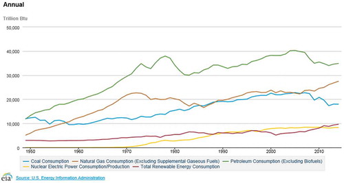
These changes in fossil fuel production, superimposed on increases in the availability of renewable sources of energy, are driving changes in the way energy is used in the United States. As shown in Figure 3, increases in the use of renewables and natural gas have been approximately equal in magnitude over the past decade and have driven decreases in the use of oil and coal (EIA, 2015d). Overall, the largest changes have been in the substitution of natural gas and renewables for coal in electricity generation (EIA, 2015e), the substitution of biofuels for petroleum use, the replacement of domestic production for oil imports, and the replacement of NGPLs for petroleum derived naphtha in chemical manufacturing.

Figure 3. Consumption of energy in the United States, by energy source, since 1949 (EIA, 2015d).

Projecting forward, changes in oil and natural gas prices will cause changes in oil and gas production in the United States, but over the long term, the U.S. Energy Information Administration has projected that increased domestic production of natural gas, natural gas plant liquids, and oil will persist for decades, and that the United States may become a net energy exporter over the next two decades (EIA, 2015f).

Although the availability of abundant, lower-cost, and domestically sourced oil, natural gas, and NGPLs has had significant economic benefits, the environmental impacts associated with increased oil and natural gas production, particularly production using horizontal drilling and hydraulic fracturing, have made these activities controversial. Among the environmental consequences of increased oil and gas production are impacts on land use, impacts on water use (Nicot and Scanlon, 2012), water contamination (U.S. Environmental Protection Agency [EPA], 2012; Osborn et al., 2011; Vidic et al., 2013; Rahm and Riha, 2012), criteria air pollutant and air toxics releases (McKenzie et al., 2012; Litovitz et al., 2013; Pacsi et al., 2013, 2015), and greenhouse gas emissions (Laurenzi et al., 2013; Miller et al., 2013; Brandt et al., 2014; Balcombe et al., 2015). Given the potential scope and magnitude of the economic and industrial transformations that increased oil and gas production can lead to, it is important to understand, as thoroughly as possible, the environmental implications of the transformations. This Critical Review will focus on the air quality implications of the production, processing, and distribution of oil and natural gas in the United States. In addition to reviewing the state of knowledge of emissions directly from oil and gas production, processing, and distribution, several case studies will examine the changes in emissions associated with changes in fuel use that have accompanied the increase in production. Three types of air pollutants will be considered: greenhouse gases, photochemical air pollutants and their precursors, and air toxics; the review will be organized into major sections on emissions, regional air quality impacts, life cycle impacts, and potential emission management strategies.

Atmospheric emissions from oil and natural gas supply chains

Overall magnitudes of atmospheric emissions

Atmospheric emissions from the natural gas and petroleum sectors are distributed along oil and natural gas supply chains, which are mapped in Figures 4 and 5. The supply chains for petroleum and natural gas in the United States differ significantly in their features. For example, the natural gas supply chain relies primarily on domestic production, with the net of imports and exports constituting less than 10% of total production in 2014. In contrast, the petroleum supply chain relies on approximately equal volumes of domestic production and imports, despite the recent increase in domestic production; the imports can include both crude and refined products. Because of these differences in the supply chains, the oil and gas sectors are mapped separately.

Figure 4. Natural gas supply chain in the United States (EIA, 2015c); flow data for 2014 are expressed in trillion standard cubic feet (tcf) of natural gas. Note that some gas is consumed along the supply chain (e.g., consumed in compression) and some is lost or unaccounted for.

Figure 5. Petroleum supply chain in the United States (EIA, 2015b); flow data for 2014 are expressed in billions of barrels (billion bbl) of oil and quadrillion (10¹⁵) BTU. (*Energy content depends on product type; for example, 1 Quad is equivalent to 0.19-0.21 billion bbl of refined gasoline, and 0.17-0.18 billion bbl of diesel).

As shown in Figure 4, the natural gas supply chain, delivering gas to end users, consists of five major segments: (i) production; (ii) gathering; (iii) processing; (iv) transmission and storage; and (v) distribution. The boundaries between some of these supply chain segments are well defined. For example, the transmission sector provides gas to distribution networks serving residential, commercial, and small industrial users, at a well-defined point called a city gate. In contrast, the boundary between production and gathering is not well defined. In some locations, gathering operations perform some combination of preliminary compression, dehydration, and treatment of well-head gas (Mitchell et al., 2015). At other locations, some of that processing occurs at a well site or at a gas processing facility, blurring the boundaries between these segments of the supply chain. In addition, the total volume of material flowing through various parts of the natural gas supply chain varies. For example, some natural gas production yields pipeline quality gas, without the need for additional gas processing; consequently, the volume of gas in the processing sector is only about 60% of the volume produced. Similarly, some gas flows directly from regional transmission lines to large users, such as electricity generating units (power plants), so flow through the distribution network is less than through the transmission network.

In contrast to the natural gas network, where the supply is primarily domestic, in the petroleum supply chain, more than half of the petroleum used in the United States is imported. In addition, petroleum processing facilities are more centralized than gas processing facilities. In contrast to the roughly 500 gas processing facilities (EIA, 2015g), located in natural gas production regions and with a wide range of capacities (EIA, 2015c), petroleum refining is concentrated in approximately 140, generally large-capacity, facilities, concentrated in a few locations (EIA, 2015b). As with the natural gas system, flows of crude oil and refined products through the petroleum supply chain varies; in this case, the flow variations are driven by flows of imports. For example, the total volume of crude oil processed by U.S. refineries in 2014 (3.95 billion barrels) exceeded the total volume of oil produced domestically (3.18 billion barrels).

Although the natural gas and petroleum supply chains have distinctive features, they are also increasingly linked, since many domestic oil wells now produce both oil and natural gas (associated gas) and many gas wells produce liquid products (condensate and oil). Although definitions vary, a well with a rate of oil production greater than 1 barrel per 12,500 standard cubic feet (scf) of gas production is typically referred to as an oil well. Wells with lower hydrocarbon liquids production are referred to as gas wells.

Natural gas plant liquids (NGPLs; ethane, propane, and butanes) are produced at natural gas plants. These high-volatility hydrocarbons leave the well sites with the gas product, but are subsequently separated into individual chemical product streams. Where the separation (fractionation) occurs varies, in some cases occurring close to production operations, and in other cases occurring after transport.

As production of oil and gas in the United States has increased over the past decade, estimated magnitudes of emissions of criteria air pollutants, specifically volatile organic compounds (VOCs) and nitrogen oxides (NO_x), reported through the EPA’s National Emission Inventory (EPA, 2015a), have increased significantly, beginning their increase in 2005 (see Table 1 and Figure 6). Between 2005 and 2011, the year of the most recent National Emission Inventory (version 2), VOC emissions from petroleum and related industries reported through the National Emission Inventory increased by almost 400%, due to both increased activity and more comprehensive reporting. In 2011, the 2.77 million tons/year of VOC emissions from the petroleum and related industries sector represented 16% of the 17 million tons per year of total anthropogenic VOC emissions in the United States. Estimated emissions of NO_x increased by 94% between 2005 and 2011, for similar reasons, and the sector’s 0.68 million tons of emissions in 2011 represented 4.7% of the 14.5 million tons of anthropogenic NO_x emissions in the United States.

Table 1. Emissions of criteria pollutants and greenhouse gases from the oil and gas supply chain

Emission parameter	VOCs	NOx	Greenhouse Gases
Emissions from oil and gas sector in most recent emission inventory	2.77 million tons (2011 NEI; EPA, 2015a)	14.5 million tons (2011 NEI; EPA, 2015a)	226.4 million metric tons CO2e (2013 GHGEI; EPA, 2015c)
Percentage of total US anthropogenic emissions accounted for by the oil and gas sector	16%	4.7%	3.4%
Rate of change of emissions (2002–2011)	Increased by 400% compared with decrease of 11% in total anthropogenic emissions	Increased by 94% compared with decrease of 40% in total anthropogenic emissions	Decreased by 5% compared with decrease of 5% in total anthropogenic emissions

Figure 6. Oil and gas production compared to emissions of VOCs, NO_x, and greenhouse gases from the petroleum and natural gas supply chains (2002–2011); all data normalized by 2002 levels.

In contrast to the increasing estimates of emissions of criteria air pollutants, estimated emissions of greenhouse gases, primarily carbon dioxide and methane, from the oil and natural gas sector have been decreasing over the same period. These contrasting trends for VOC, NO_x, and greenhouse gas emissions are shown in Figure 6 and Table 1. Greenhouse gas emissions from the oil and gas sector reported in Figure 6 are on a carbon dioxide equivalent (CO₂e) basis. For carbon dioxide, emissions in CO₂e are equal to the mass of carbon dioxide emitted. For methane, the CO₂e is based on the mass of methane emitted multiplied by a Global Warming Potential (GWP). The GWP for a gas is a measure of the total energy that a gas absorbs in the atmosphere over a particular period of time (usually 100 years), compared with carbon dioxide. For methane, the 100-year GWP used in current EPA greenhouse gas reporting is 25, which means that methane mass emissions are multiplied by 25 to arrive at the emissions expressed as CO₂e.

In the United States, there are two primary sources of public information on greenhouse gas emissions from the oil and natural gas sector. The EPA Greenhouse Gas Reporting Program (GHGRP) (EPA, 2015b) provides annual estimates of greenhouse gas emissions from individual oil and gas production and processing facilities that exceed a threshold quantity of emissions. A complementary data source is the EPA’s Greenhouse Gas Emission Inventory (GHGEI) (EPA, 2015c), which provides emission data aggregated by region, and attempts to account for all sources. Although somewhat redundant with GHGRP data, the GHGEI is based on different information and provides an independent emission estimate. Both sources of greenhouse gas emission estimates will be used in this review; the GHGEI will be used in estimating national totals because it is comprehensive; the GHGRP will be used in examining the distribution of emissions among facilities and sources.

The total emissions of greenhouse gas reported through the EPA GHGEI for 2013 (released in 2015; EPA, 2015c) for natural gas and petroleum systems was estimated as 226.4 million metric tons of CO₂e, not including end-user combustion of the fuel products. This represents 3.4% of the U.S. total for anthropogenic greenhouse gas emissions (6673 million metric tons CO₂e). This is a lower percentage than the fraction of anthropogenic VOC emissions accounted for by the oil and natural gas sector (17%), but is comparable to the fraction of total anthropogenic NO_x emissions accounted for by the sector (4.7%). To better understand these distributions in emissions, it is useful to further characterize the emissions by source category.

Greenhouse gas emission estimates can be categorized by facility type and source category using the EPA GHGRP. As shown in Table 2, the EPA GHGRP for 2013 (released in 2015; EPA, 2015b) reports a total of 224 million metric tons of CO₂e, which is within 1% of the 226 million tons of emissions reported through the EPA GHGEI. Emissions reported through the GHGRP are dominated by the onshore production, natural gas processing, and natural gas transmission portions of the oil and gas supply chains. Approximately a third of the greenhouse gas emissions (on a CO₂e basis) are due to methane, and most of the methane emissions are attributed to production operations. The emissions can be further disaggregated to specific sources, as shown in Table 3. The reductions reported in greenhouse gas emissions over the past decade, as contrasted with the increases in VOC and NO_x emissions, can be attributed in large part to decreases in emissions of methane, especially in production operations. For example, emission reductions from just two production source types, well completions and liquid unloadings (described in more detail later in this review), accounted for approximately 800 kilotons of methane emission reductions, or approximately 20 million metric tons of CO₂e (EPA, 2015c).

Table 2. 2013 reported greenhouse gas emissions by industry segment (EPA, 2015d)

Industry Segment	Number of Facilities	Emissions (Million Metric Tons CO2e)	Percentage of Emissions Due to Methane (as CO2e)
Onshore production	503	95	52%
Offshore production	107	6	17%
Natural gas processing	433	59	7%
Natural gas transmission	487	23	22%
Underground natural gas storage	48	1
Natural gas distribution	173	15	100%
LNG import/export	8	<1
LNG storage	5	<1
Other oil and gas combustion	415	25	0%
Total	2164	224	33%

Notes: Total number of facilities is smaller than the sum of facilities from each segment because some facilities reported under multiple segments. A facility is included in the count of number of facilities if it reported emissions (even if the reported emissions were zero) under a given segment; in addition, facilities may include multiple individual sites; for example, a single company’s report for a production region can consist of many well sites.

Table 3. 2013 reported greenhouse gas emissions by source type (EPA, 2015d)

Source	Emissions (Million Metric Tons CO2e)	Emissions Due to Methane (Million Metric Tons CO2e)
Pneumatic devices	25	25
Acid gas removal units	13	0
Associated gas venting and flaring	12	2
Equipment leaks	10	10
Distribution mains	9	9
Other flare stacks	8	1
Atmospheric tanks	4	2
Liquids unloading	4	4
Distribution services	4	4
Reciprocating compressors	4	4
Pneumatic pumps	3	3
Gas well completions and workovers	3	2
Blowdown vents	2	2
Offshore sources Centrifugal compressors	1	1
Dehydrators	2	2
Distribution stations	1	1
Well testing	1	0
Total	106	72

Many of the source categories shown as important for greenhouse gases, shown in Table 3, will be less important or negligible for VOCs and NO_x. To understand differences in source categories and the differences in national trends for emissions (Figure 6), it is useful to consider case studies of specific production regions. This review will use data from the Barnett Shale and Eagle Ford Shale oil and gas production regions in Texas as case studies.

Overall magnitudes of emissions: Case studies of individual production regions

The Barnett Shale oil and gas production region in North Central Texas has seen natural gas production grow from 0.11 billion cubic feet per day (bcf/day) in 2000, to over 5 bcf/day in 2011 (Medlock, 2012; Texas Railroad Commission, 2015). In 2011, production from the Barnett Shale represented approximately 7% of the 70 bcf/day of total natural gas withdrawals in the United States, making the Barnett Shale one of the largest natural gas production regions in the United States. The production region includes 24 counties north and west of Fort Worth, with a total of more than 20,000 producing oil and gas wells (Texas Commission on Environmental Quality [TCEQ], 2012). Although new wells continue to be drilled, the field as a whole has likely reached its peak rate of natural gas production (University of Texas Bureau of Economic Geology [UT BEG], 2013), and production fell from 5.7 bcf/day in 2011 to 4.4 bcf/day in 2015 (Texas Railroad Commission, 2015). Production is expected to continue over the next several decades, eventually totaling approximately 50 trillion scf (UT BEG, 2013).

The Eagle Ford Shale oil and gas production region in south Texas has seen rapid development since 2008. Natural gas production in the Eagle Ford Shale increased from 0.002 bcf/day in 2008, to more than 7 bcf/day in 2015 (EIA, 2015h). In addition to natural gas, many of the wells in the region produce significant quantities of NGPLs and oil. The Eagle Ford Shale extends, northeast to southwest, over hundreds of kilometers from near San Antonio to south of the Mexican border.

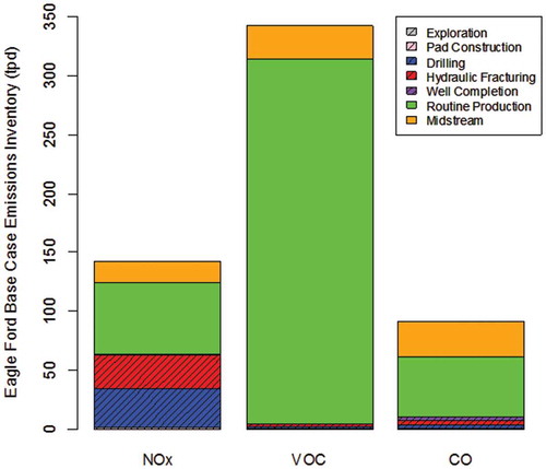
Criteria air pollutant emissions for the Barnett and Eagle Ford shales provide similarities and contrasts, due to differences in the stage of development of the two production regions. VOC emission inventories in both regions are dominated by emissions from tanks; these emissions are associated with the production of liquid hydrocarbon products. In contrast, NO_x emissions in the Eagle Ford have significant components associated with both preproduction (e.g., drilling and hydraulic fracturing) and production activities. The distinction between preproduction and production sources is important because preproduction emissions occur only during the first few months of a well’s 20–30-year life cycle. NO_x emissions from engines used in drilling and hydraulic fracturing dominate the preproduction emissions. Figure 7 shows estimated emissions of VOCs, CO, and NO_x, for the Eagle Ford Shale in 2012, a period when new well development was extensive (Alamo Area Council of Governments [AACOG], 2013; Pacsi et al., 2015); preproduction sources accounted for 45% of NO_x, 1% of VOCs, and 11% of CO emissions.

Figure 7. Source categories of estimated emissions of NO_x, VOCs, and CO, in 2012, from oil and gas production sources in the 25 counties of the Eagle Ford shale (Pacsi et al., 2015).

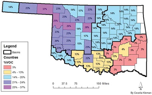
Estimated greenhouse gas emissions show a different pattern of sources than either VOCs or NO_x. As shown in Table 3, the largest single source of greenhouse gas emissions along the oil and gas supply chains is estimated to be natural gas venting from pneumatic controllers. Pneumatic controllers use gas pressure to control the operation of mechanical devices, such as valves, and either continuously or intermittently emit gas. When natural gas produced at a site is used as the high-pressure gas supply for a controller, venting of methane, ethane, and smaller amounts of VOCs result from controller operation. Thus, this largest source of greenhouse gas emissions along the natural gas and petroleum supply chains is often (but not always) a moderate source of VOCs and is not a source of NO_x. Similarly, the largest source of VOC emissions in the Barnett Shale and Eagle Ford Shale oil and gas production regions (see Figure 7 and Table 4), hydrocarbon storage tanks, is a relatively small source of greenhouse gas emissions (when systems are operating correctly) and is not a source of NO_x. Tanks, particularly well site hydrocarbon storage tanks, are not a dominant source of greenhouse gas (methane) emissions because the amount of methane that can be emitted by a properly operating tank is limited to the methane dissolved in the hydrocarbon liquids sent to tanks. Dissolved methane will rapidly flash from a tank operating at ambient conditions; in contrast, moderately volatile hydrocarbons will be emitted from a tank nearly continuously, driven by changes in tank level and diurnal temperature variations. Not all production regions have the same emission patterns, however. Also shown in Table 4 are VOC emissions reported for production regions in Oklahoma (Gibbs, 2015), where pneumatic controllers are estimated to be the largest VOC source. A qualitative comparison of dominant sources of VOCs, NO_x, and greenhouse gases (largely methane) is provided in Table 5. Given these varied sources of emissions, it is not surprising that overall trends in emissions for greenhouse gases, VOCs, and NO_x (Figure 6) can be quite different.

Table 4. Percentage of total VOC emissions by source type, as reported in the Barnett Shale (Zavala et al., 2014) and in Oklahoma (Gibbs, 2015)

Source Type	Barnett Shale	Oklahoma
Condensate and oil tanks	54.9% + 1.2%	20.3%
Fugitives	20.6%*	14.2%
Pneumatic devices and pumps	*	44.1%
Liquids unloading		9.0%
Without source type	8.1%
Water tank	6.8%
Engine	3.9%	0.4%
Loading	2.7%	2.1%
Separator	0.8%
Vent	0.4%
Glycol dehydrator	0.4%	2.5%
Degassing		4.8%
Compressors		0.6%
Associated gas		0.6%
Flare	0.1%
Fracturing and completions	<0.1%	1.0%
Amine unit	<0.1%
Heater	<0.1%
Boiler	<0.1%
Other	<0.1%

Notes: *Pneumatic devices may be included in fugitives in the Barnett Shale data, but are likely underrepresented, as described in Zavala et al. (2014).

Table 5. Major sources of inventoried emissions for greenhouse gases, VOCs, and NO_x

Greenhouse Gases	VOCs	NOx
Pneumatic controllers, pumps Gas treatment Flaring Compressors Leaks Liquid unloadings	Tanks, loading operations Leaks Pneumatic controllers, pumps Engine operations	Drilling and fracturing Compression Process heaters

Notes: *Source strengths can vary over time and from region to region.

Spatial and temporal variability in emissions

Temporal variability in emissions

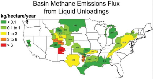
The most commonly used VOC, NO_x, and greenhouse gas emission inventories for the petroleum and natural gas sectors (EPA, 2015a, 2015b, 2015c) report annual emission rates. This annual reporting can mask significant temporal variability in emissions. The NO_x emissions reported in Figure 7, segregated into preproduction and production emissions, are an example of temporal variations driven by the life cycle of a well. In this case, NO_x emissions due to energy consumption in drilling and hydraulic fracturing of wells is a significant contributor to NO_x emissions in a rapidly expanding oil and gas production region, the Eagle Ford Shale in south Texas. These preproduction emissions are smaller in the Barnett Shale oil and gas production region in North Central Texas, where the rate of new well drilling and fracturing is not as rapid. Similarly, for VOCs and greenhouse gases, there are activities that occur early and late in a well’s life cycle, which can influence which sources are important in estimating emissions. Completion flowbacks, which occur after a well has been fractured and clear a well of fracturing fluid to enable production, can be significant contributors to VOC and greenhouse gas emissions in regions where new wells are being added. Emissions of VOCs and greenhouse gases from liquid unloadings can be significant in more mature production regions. Liquid unloadings clear liquids that can accumulate in a well bore during production; liquid unloadings can, in some operations, lead to venting of produced gas. These emissions can be a large fraction of total greenhouse gas and VOC emissions in regions such as the San Juan Basin in the Four Corners region, where large numbers of mature wells with relatively low pressure and high liquids production are in operation. This temporal variability in emissions can also lead to spatial variability in emissions as fields age. Figure 8 shows a mapping of emissions from liquid unloadings, illustrating a regional concentration in emissions in the relatively mature San Juan production region in the Four Corners area (Pacsi and Harrison, 2015).

Figure 8. Spatial variability in liquid unloading emission rates (Pacsi and Harrison, 2015).

Changes in the types of operational activities, and emissions, occurring in oil and gas production regions, change over time scales of months to years. Some temporal emission variability occurs over much shorter time scales, however. In some cases, emissions can change over time periods as short as minutes. Some short-duration events occur by design. For example, liquid unloadings can last for periods as short as a few minutes, yet during that period have emission rates equivalent to a thousand or more wells in routine operation (Allen et al., 2015b). Emissions can also be due to unplanned events. One prominent recent example of a large unplanned emission event is the well blowout in a natural gas storage facility in California. This large leak had emissions that reached a peak of 60 metric tons of methane per hour (Conley et al., 2016), a methane emission rate, from a single point, that is roughly equivalent to the routine emissions from tens of thousands of wells in the Barnett Shale (Lyon et al., 2015; Zavala et al., 2015c). This leak persisted for several months and is estimated to have released 97,100 metric tons of methane (97.1 Gg; 2.4 million metric tons of CO₂e); an amount equivalent to 1% of the annual emissions from the oil and natural gas supply chains (Conley et al., 2016).

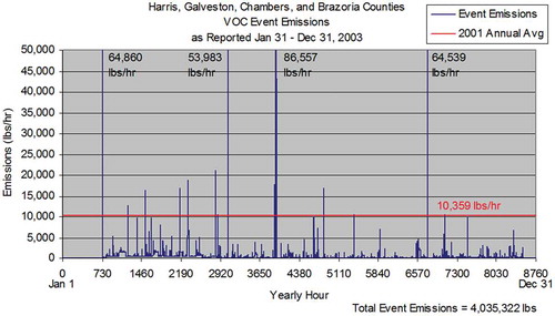
Data are sparse on the frequency and magnitude of unplanned releases; however, one source of data is an emission event reporting system for major downstream emission sources maintained by the State of Texas (TCEQ, 2015a). Murphy and Allen (2005) reported that individual VOC emission events from refineries and chemical manufacturing facilities in the Houston-Galveston region, reported through the State of Texas database, can exceed 10,000 lb/hr, a rate equivalent to the annual average rate of VOC emissions from the thousands of individual industrial sources in the entire region. A time series for the first year of operation of the emission event reporting system is shown in Figure 9. Although these short-lived events represented less than 10% of total annual VOC emissions from refining and chemical manufacturing in the Houston-Galveston region, during the periods when they occur, they can dominate total emissions and atmospheric photochemistry (Webster et al., 2007; Vizuete et al., 2008).

Figure 9. VOC emission events in the Houston-Galveston region. Data are shown for the first year of reporting by hour (8760 hr in a year); the horizontal red line shows the level of the annual average VOC emissions from all industrial sources in the Houston-Galveston region; multiple hours during the year include emission events where releases from a single facility exceed annual average emissions from all facilities in the region (Murphy and Allen, 2005).

Spatial variability in emissions

Spatial variability in emissions from oil and natural gas supply chains can occur for a variety of reasons, including the reservoir characteristics of a production region, the types of activities being performed in a region, the nature of the oil, gas, and liquids being produced, processed, and transported, the emission regulations in place in a region, and other factors. As an example of variability in emissions between basins, using aircraft measurements, Peischl et al. (2015) have reported very different methane emission rates in different natural gas production regions, ranging from a low of 0.18–0.41% of gas production in the northeast Marcellus Shale (Pennsylvania) to rates of 1.0–2.1% in the Haynesville Shale (East Texas) and 1.0–2.8% in the Fayetteville Shale (Arkansas). Using the same type of aircraft-based measurements, emission rates as high as 6.2–11.7% of natural gas production have been reported in the Uintah production region in Utah (Karion et al., 2013). Similarly, Zavala et al. (2015a), using measurements of emissions from individual pieces of equipment at hundreds of sites throughout the United States, reported methane emission rates, normalized by rates of natural gas and oil production, that differed by more than an order of magnitude across regions. Studies reporting this interregion emission variability are summarized in Table 6.

Table 6. Spatial variability in emissions reported in recent methane emission studies

Region Studied	Citation	Method for Measuring Ambient Concentrations	Normalized Emission Rate or Comparison with Bottom-Up Inventories	Method Used for Attributing Methane Emissions
Southwestern Marcellus	Caulton et al., 2014b	Aircraft-based measurements downwind of production region (but not upwind); methane measured using high-precision, high-time-resolution instruments. Some measurements of single production sites	Observed emission rate, with uncertainties (0.18–1.2 Tg/yr), found to be within range of bottom-up inventory	Emissions compared with oil and gas inventories
Unitah Basin	Karion et al., 2013	Aircraft-based measurements upwind and downwind of production regions; methane measured using high-precision, high-time-resolution instruments, absorption spectrometry at precise infrared wavelengths; light alkanes analyzed from discrete air samples	Emissions (0.48 ± 0.13 Tg/yr) 6.2–11.7% of natural gas production	Bottom-up inventories for cattle and gas seepage were subtracted from total emissions; difference assigned to oil and gas activity based on methane to light-alkane ratios
Barnett Shale	Karion et al., 2015	Aircraft-based measurements upwind and downwind of production regions; methane measured using high-precision, high-time-resolution instruments, absorption spectrometry at precise infrared wavelengths	Emissions reported as 0.66 ± 0.11 Tg/yr; reported as 1.5% of gas production by Zavala et al. (2015c)	See Smith et al. (2015)
Four Corners region	Kort et al., 2014	Satellite measurements used with atmospheric models to infer concentrations and emission rates of methane	Emissions reported as 0.59 (0.50–0.67) Tg/yr; EPA GHGRP estimates cited as 0.33 Tg/yr	Differences between inventories and inferred emission rates based on satellite measurements attributed to “established gas, coal, and coalbed methane mining and processing”
Los Angeles	Peischl et al., 2013	Aircraft-based measurements of methane, carbon dioxide (CO2), carbon monoxide (CO), and C2–C5 alkanes using high-precision, high-time-resolution instruments	Emissions from all sources reported as 0.41 ± 0.04 Tg/yr, with 0.032 Tg/yr assigned to natural gas and 0.19 Tg/yr assigned to seeps or pipeline gas	Bottom-up inventories of CH4, CO, and CO2 are used to determine ratios of CO/CO2, CH4/CO, and CH4/CO2 from the inventories. The top-down measurements of the ratios are compared with the inventories and missing emissions are inferred
Northeast Marcellus, Haynesville, and Fayetteville shales	Peischl et al., 2015	Aircraft-based measurements upwind and downwind of production regions; methane measured using high-precision, high-time-resolution instruments, absorption spectrometry at precise infrared wavelengths	Emissions (percentage of gas production) 0.18–0.41%, 1.0–2.1%, and 1.0–2.8% in the northeast Marcellus, Haynesville, and Fayetteville shales (0.11, 0.65, and 0.31 Tg/yr)	Total methane emissions quantified for each region; emissions from sources other than oil and gas operations subtracted from total emissions to arrive at estimate of emissions from oil and gas sources
Denver-Julesburg	Pétron et al., 2012	Daily samples collected at fixed ground site (NOAA Boulder Atmospheric Observatory); methane and light alkanes analyzed	2.9-7.7% of natural gas production	Automobile-based measurements of oil and gas emissions used to establish emission rates, which were then extrapolated to region wide estimates
Denver-Julesburg	Pétron et al., 2014	Aircraft-based measurements upwind and downwind of production regions; methane measured using high-precision, high-time-resolution instruments, absorption spectrometry at precise infrared wavelengths	Emissions of methane 3 times higher than GHGRP reports (0.17 ± 0.06 Tg/yr)	Total methane emissions quantified for each region; emissions from sources other than oil and gas operations subtracted from total emissions to arrive at estimate of emissions from oil and gas sources
Los Angeles	Wennberg et al., 2012	Aircraft-based measurements of methane, carbon monoxide (CO), and ethane	Emissions from all sources reported as 0.44 ± 0.15 Tg/yr	Bottom-up inventories of CH4 and CO are used to determine ratio of CH4/CO. The top-down measurements of the ratio is compared with the inventories and missing emissions are inferred and assigned to natural gas systems, based on methane to ethane ratios and assuming all ethane is due to natural gas systems
Multiple U.S. production regions	Zavala et al., 2015a	Emissions estimated based on bottom-up equipment measurements	For production only (no gathering, processing, transmission or distribution); omissions attributed to natural gas 0.07–0.60% of production	Counts of equipment per well multiplied by numbers of wells, and normalized by production; methane emissions attributed to multiple products (natural gas, oil, NGPLs)

Although a number of studies have identified differences in emission rates between production regions, variability in emissions within production regions is less well recognized. This intraregion variability is largely driven by differences in the composition of the produced fluids. As an example, the Barnett Shale oil and gas production region in North Central Texas has regions that produce dry gas (no or very limited liquid hydrocarbons produced) and regions that produce wet gas (hydrocarbon liquids production). Therefore, different parts of the production region have different types of equipment on well sites, leading to different emission rates and compositions. Figure 10 characterizes the spatial variability by mapping methane to ethane emission ratios, methane to propane emission ratios, and methane emissions (Zavala, 2014). Figure 11 shows similar spatial variability for Oklahoma (Gibbs, 2015).

Figure 10. Spatial variability in (a) methane to ethane emission ratios (C1:C2, by mass); (b) methane to propane emission ratios (C1:C3, by mass); and (c) methane emissions from the Barnett Shale production region in North Central Texas (Zavala, 2014).

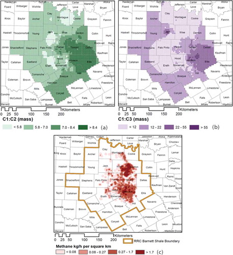
Figure 11. Percentage of VOCs in produced gas (and fugitive emissions) in Oklahoma, as documented in permit data.

Overall, national and regional emission inventories illustrate the complexity of emissions from the petroleum and natural gas sector. Major emission sources differ for VOCs, greenhouse gases, and NO_x. The spatial patterns of emissions vary, not only by production region, but also over length scales as small as a few kilometers. Emissions also vary over time, with some variability occurring over months to years, but other types of variability occurring over minutes to hours.

Comparisons of emission estimates with measurements

National and regional inventories of emissions from petroleum and natural gas sources, of the type summarized in Figures 6–11 and Tables 1–5, are based on emission estimates. Emissions are generally estimated by multiplying an average emission measurement for a device (e.g., a pneumatic controller) or operation (e.g., a liquid unloading) by the number of times that emission occurs on the national scale. Generally, the emission measurement is referred to as an “emission factor” or EF, and the data used to scale up the emissions are called the activity factor (AF). Emissions are calculated as

(1)

where EF_i is the emission factor for region I; AF_i is the activity factor for region I; and ER_i is the resulting emission rate total for region i.

Emission inventories estimated in this way are often referred to as “bottom-up” emission estimates, and the estimates are subject to uncertainties in both activity factors and emission factors. Recent field studies have sought to quantify these uncertainties. For example, Allen et al. (2015a) assessed differences between observed and inventoried pneumatic controller activity factors and reported a factor of 2–3 difference between observed numbers of pneumatic controllers per well (2.7 controllers per well) and the average number of controllers per well in the U.S. Greenhouse Gas Emission Inventory (1.0 controllers per well). Similar results have been reported in a study by the State of Oklahoma, which found 3.6 pneumatic controllers per well (Gibbs, 2016).

In addition to uncertainties due to activity data, differences between observed emission factors and emission factors used in inventories have also been reported. Emission factors, based on recent observations, which are both higher and lower than emission factors used in inventories, have been reported. For example, Allen et al. (2013) reported average emissions per completion flowback that were substantially lower than average emissions per completion in EPA’s GHGEI for 2011 (inventory at the time the work was done). Allen et al. (2013) also reported average emissions per well from leaks that were higher than the EPA GHGEI for 2011. Similarly, Lamb et al. (2015) reported emissions for plastic pipes in distribution networks that were significantly lower than emission factors in current use, whereas McKain et al. (2015) reported emissions for the Boston natural gas distribution and use network that were significantly higher than emission estimates in current inventories. Moving beyond emissions associated with specific equipment, bottom-up emission estimates for a region may omit sources from the inventory, such as abandoned wells or episodic emission events.

To summarize, national and regional emission inventories estimated using emission factors and activity factors (bottom-up emission estimates) can have uncertainties due to inaccurate activity data, inaccurate emission factors, malfunctioning or improperly operated equipment, and missing sources. To assess uncertainties, bottom-up national or regional emission inventories are often compared with measurements that infer emissions based on ambient concentrations (Allen, 2014a, 2014b). Atmospheric concentrations of pollutants measured or inferred from ground, aircraft, and satellite platforms can be used to infer (using atmospheric models and assumptions) emissions in a region in a process referred to as a “top-down” analysis. For example, for aircraft measurements, the difference between average concentrations of a pollutant upwind and downwind of a region can be used, with the ventilation rate of the region, to estimate regional emissions. The next section of the Critical Review will summarize the state of knowledge regarding uncertainties in emission inventories based on a variety of top-down measurements. Many of the most recent measurements have focused on greenhouse gas (especially methane) emissions; therefore, much of the analysis will focus on methane emissions. However, some data collected over the past decade suggest that some of the same factors are important in assessing the uncertainties in criteria air pollutant emissions, and studies reporting these data will be briefly summarized.

Differences between top-down and bottom-up inventories of methane emissions

Recent reviews (Miller et al., 2013; Brandt et al., 2014) have concluded, based on top-down methane emission assessments, that bottom-up inventories underestimate or omit sources of methane emissions. For example, Brandt et al. (2014) report that missing or underestimated sources of methane emissions in the U.S. national emission inventory total 14 Tg/yr (7–21 Tg/yr), which is approximately 50% (25–75%) of the total anthropogenic emissions for the United States.

In general, these differences between emissions inferred from top-down measurements and emissions inventoried using bottom-up estimates have been attributed to missing or underestimated emissions from oil and gas operations. The methods used to attribute the missing emissions to oil and gas operations vary. When top-down studies are performed in a region in which one source dominates, bottom-up estimates of other emission sources are sometimes subtracted from the total emissions to arrive at estimates of the emissions of the dominant emission source for the region. For example, to obtain methane emissions from oil and gas production in the Haynesville, Fayetteville, and Marcellus shale regions, Peischl et al. (2015) subtracted bottom-up methane emissions from non–oil and gas sources from the total methane emissions (determined using top-down methods) for the regions. In other cases, a molecular tracer is used to attribute methane emissions to a source that dominates the emissions of that tracer. For example, ethane is often used as a molecular tracer for oil and gas emissions, along with the assumption that ethane is only emitted from oil and gas sources. Smith et al. (2015) used ethane to methane ratios to attribute the fraction of the methane emissions in North Central Texas that are attributable to oil and gas production activities in the Barnett Shale, assuming that all of the observed ethane emissions were due to oil and gas operations. Table 6 provides a summary of the methods used in recent studies to attribute emissions to sources.

Based on these source attribution approaches, most top-down studies of methane emissions have concluded that emissions from petroleum and natural and gas supply chains are underestimated using bottom-up methods. To identify the causes of these underestimates, a number of field studies have been performed, and the findings from these recent field programs are summarized in Table 7. Although uncertainties associated with activity data and missing emission source types can be significant in some situations (e.g., counts of pneumatic controllers may have been underestimated in recent inventories and emissions from abandoned wells are not included in most inventories), the dominant finding emerging from most recent studies has been that a small group of sources contributes a large fraction of emissions. Collectively, these sources have been referred to as “super-emitters.”

Table 7. Measurement studies assessing accuracy of bottom-up emission inventories in the natural gas supply chain

Geographical Region Sampled	Devices Sampled	Activity Factor	Emission Factor	High-Emitting Subpopulations	Reference
Natural gas production sites
U.S. National sample	Well completions, unloadings, leaks, pneumatic pumps and controllers		Emission factors for leaks and pneumatic controllers higher than in EPA GHGEI; emission factors for well completions lower than in GHGEI	Observed for unloadings, pneumatic controllers	Allen et al., 2013
British Columbia	Pneumatic controllers		Emissions reported separately for individual manufacturers; only high bleed controllers targeted Emissions averages similar to those for Allen et al. (2015a) for similar applications	Only high-bleed controllers targeted	Prasino, 2013
U.S. National sample	Pneumatic controllers	2.7 controllers per well (compared with 1.0 in EPA GHGEI)	Emissions per controller 17% higher than average in GHGEI (5.5 scf/hr whole gas, 4.9 scf/hr methane)	19% of controllers accounted for 95% of national emissions from pneumatic controllers	Allen et al., 2015a
Oklahoma	Pneumatic controllers	3.6 controllers per well (compared with 1.0 in EPA GHGEI)	Emissions averaged 1.05 scf/hr whole gas for all devices	3.5% of controllers accounted for 73% of controller emissions	Gibbs, 2015
U.S. national sample	Liquid unloadings	Unloading events	Average emissions equivalent to those reported in EPA GHGEI	2–3% of wells account for more than half of national unloading emissions	Allen et al., 2015b
Marcellus Shale	Flare		Very high combustion efficiencies (>99.5%) for a single well completion flare; bottom-up inventories generally assume 98% efficiency		Allen et al., 2013
Marcellus Shale, Bakken Shale	Flares		All flares were >99.80% efficient at the 25% quartile; bottom-up inventories generally assume 98% efficiency		Caulton et al., 2014a
Natural gas gathering and processing operations
U.S. National sample	Downwind sampling of sites		Emissions averaged 0.20% of throughput for gathering facilities and 0.075% for processing facilities	Some gathering facilities had emissions that were in excess of 10% of gas throughput and 30% of gathering facilities contribute 80% of the total emissions; all processing facilities had emissions <1% of throughput	Mitchell et al., 2015; Zimmerle et al., 2015
Natural gas transmission and storage
U.S. National sample	Downwind sampling of sites, with on-site measurements and emission estimates		Emission factors both higher and lower than inventory factors observed; largest emission factor from open ended lines (measurements >factor of 5 greater than GHGRP emission factor)	Highest-emitting 10% of sites (including two super-emitters) contributed 50% of aggregate methane emissions	Subramanian et al., 2015
Natural gas distribution, metering and regulating (M&R)
13 urban distribution systems	Direct sampling of emissions		Emissions of 0.10–0.22% of the methane delivered, equivalent to 36–70% less than the 2011 EPA GHGEI; emission factors reported for multiple types of pipes and for M&R facilities, multiple pressures	Large reductions in emissions from high-emitting facilities, compared with measurements made in early 1990s (Harrison et al., 1996)	Lamb et al., 2015
Boston	Centralized monitors on tall buildings		2.7 ± 0.6% of natural gas use, also including urban end-use emissions		McKain et al., 2015

The concept of a “super-emitter” classification in emission inventories is not new. It has been known for decades that roughly 10% of the passenger car fleet in the United States contributes roughly 50% of all on-road emissions (Stedman, 1989; National Research Council, 2001). The situation for many source types in the petroleum and natural gas supply chains is analogous. For example, the EPA reports that approximately 50,000 wells in the United States vent during liquid unloadings, resulting in 259 Gg/yr of methane emissions (EPA, 2015c). A small fraction of these venting wells, perhaps 3–5%, likely accounts for half of unloading emissions (Allen et al., 2015b). Similarly, multiple studies (Prasino 2013; Allen et al., 2015a; Gibbs, 2015) have found that a small subpopulation of pneumatic controllers (the largest source of greenhouse gases in the petroleum and natural gas supply chains) dominates emissions. Allen et al. (2015a), for example, estimated that 20% of pneumatic controllers in a national sampling of natural gas sites account for 95% of pneumatic controller emissions, and Gibbs (2015) found that 3.5% of controllers accounted for 73% of controller emissions at sites sampled in Oklahoma.

A significant issue, which has not yet been completely resolved, is why sources are or become super-emitters. Again, analogies with vehicle emissions can provide some insights. Large numbers of vehicle tests have revealed that although there are some vehicles that are more likely than others to become “super-emitters,” the way in which a vehicle is operated and maintained often plays a critical role (National Research Council, 2001). Similarly, in the petroleum and natural gas supply chains, there are some sources that are more likely than others to become super-emitters, but operational practices also play a role. For example, in the source category of liquid unloadings, mature wells with low reservoir pressure and high rates of liquids production are more likely to have high unloading emissions, leading to a geographical concentration of unloading emissions (see Figure 8). In contrast, high emissions from pneumatic controllers and compressors (Allen et al., 2015a; Harrison et al., 2011) have been attributed to devices not operating as designed, and are distributed throughout the United States, and may be reduced or eliminated by equipment repair or replacement.

Another way in which super-emitters have been defined is facility or site based, rather than equipment based. Ground-level measurements, made downwind of petroleum and natural gas supply chain sites, have been made using a variety of techniques designed to infer emission rates from ambient concentrations. A procedure that enables some of the most precise measurements is generally referred to as a tracer technique (Lamb et al., 1995; Shorter et al., 1997; Kolb et al., 2004; Herndon et al., 2005, 2013; Allen et al., 2013). In this method, tracer compounds (e.g., SF₆, N₂O, C₂H₂) are released at a known rate at or near an emission source; downwind measurements of the target pollutant (minus background) and the tracers (minus background) are equal to the ratio of emission rates, if the dispersion of the target pollutant and the tracer are identical. Target pollutant emissions are estimated by multiplying the known emission rate of the tracer by the concentration ratio of the target pollutant to the tracer. If two tracers are used, the assumption of equivalent dispersion can be quantitatively tested. Tracer studies have pointed to a skewed distribution of emissions among sites, with a small number of sites accounting for a large fraction of emissions. However, these distributions must be interpreted carefully. The amount of equipment and throughput, and therefore the potential emission sources, on sites vary. For example, in a study by the City of Fort Worth (Eastern Research Group, 2011), which reports on emissions from 375 well sites in the Barnett Shale production region (sites were randomly selected from the well sites that were within the city of Fort Worth), 30% of the sites had 1 well, 63% had between 2 and 6 wells, and one site had 13 wells. Similarly, whereas 78% of the sites had between 1 and 4 tanks, 16% had more than 4 tanks, and one site had 20 tanks. The potential sources of fugitive emissions, such as valves and flanges, varied by an order of magnitude or more between sites. Ten percent of the sites had less than 62 valves, but 10% had more than 446 valves. Ten percent of the sites had 390 or less connectors (such as flanges), but 10% had more than 3571 (Eastern Research Group, 2011). Because of this heterogeneity in the equipment among sites, simple comparisons of emissions among sites, without adjustments for equipment counts or throughput on sites, should be viewed with caution. Nevertheless, it is possible to define super-emitting sites. One approach is to normalize emissions by site size or throughput. For example, Mitchell et al. (2015) made measurements downwind of natural gas gathering and processing facilities and normalized methane emissions by total gas throughput at the sites. Across all sites, emissions averaged 0.20% of throughput for gathering facilities; however, some facilities had emissions that were in excess of 10% of gas throughput, and 30% of the facilities accounted for 80% of the emissions. Zavala et al. (2015b) analyzed data taken downwind of natural gas supply chain sites in the Barnett Shale region and defined a functional super-emitting site as those with the highest proportional loss rates (methane emitted relative to methane produced or methane throughput). Using this definition, Zavala et al. reported that 77% of the methane emissions were accounted for by the 15% of the sites with the highest normalized emissions.

Super-emitters can play an important role in reconciling top-down and bottom-up methane emission inventories, as illustrated by analyses performed in the Barnett Shale oil and gas production region. In 2013, a large number of investigators performed coordinated aircraft and vehicular measurements of methane emissions in the Barnett Shale oil and gas production region, providing one of the richest data sets available for comparing top-down emission estimates and bottom-up emission inventories. A top-down estimate of emissions from oil and gas operations was 60,000 ± 11,000 (79% of total top-down emission estimate), based on the use of ethane as a tracer for oil and gas emissions (Karion et al., 2015; Smith et al., 2015). In contrast, a bottom-up analysis of emissions for the region (Lyon et al., 2015) led to an estimate of 46,200 kg/hr of methane from oil and gas operations (48,400 kg/hr including other minor geogenic sources), which is 61–63% of the region’s emissions. When super-emitters were accounted for, however, the top-down and bottom-up emission estimates converged (Zavala et al., 2015c).

Differences between top-down and bottom-up inventories of VOC emissions

Just as Miller et al. (2013), Brandt et al (2014), and many of the studies summarized in Table 6 found that top-down estimates of methane emissions in the petroleum and natural gas supply chains were generally larger than corresponding bottom-up estimates, multiple studies have reported top-down emission estimates greater than bottom-up inventories for VOCs. Some of these studies (e.g., Zavala et al., 2014) have been in oil and natural gas production regions, in locations analogous to many of the methane emission studies, but the most extensive studies of VOC emissions from petroleum and natural gas supply chains have been done in the Houston-Galveston region of southeast Texas, where petroleum refining and chemical manufacturing sources are extensive. Beginning with measurements done in 2000, it had been observed that ratios of hydrocarbons to NO_x in industrial plumes were consistently factors of 2–15, and in some isolated instances even a factor of 50 or higher, than the ratios reported in the inventories (Daum et al., 2001). Ratios of hydrocarbon to NO_x, higher than those in bottom-up emission inventories, were observed for alkanes, alkenes, and aromatics, but overall atmospheric reactivity was dominated by alkenes (Daum et al., 2003; Ryerson et al., 2003). These findings led to multiple years of efforts to identify the sources of the missing or underestimated emissions. In some cases, highly elevated hydrocarbon to NO_x ratios, compared with ratios in the emission inventories, can be due to the types of emission events reported by Murphy and Allen (2005). These emission events are generally associated with process start-ups, process shut-downs, process upsets, and other causes. In addition to large episodic emission events, continuous or nearly continuous sources of underestimated emissions have been identified as sources of the discrepancy. For example, most refineries and large chemical manufacturing operations have large-capacity flares designed to combust emergency blowdowns. In many cases these flares are also used to combust relatively small flow rates of vent gas (<1% of maximum flow) on a continuous or near-continuous basis (Pavlovic et al., 2012). Large-capacity flares can fail to achieve desired combustion efficiencies at low flow rates, depending on operating practices. In full-scale tests of flare operation, Torres et al. (2012a, 2012b) found that large-capacity flares, operated at low flow, have narrow operation ranges (rates of air or steam assist) in which high combustion efficiency and low smoke formation are both achieved. If a flare has too much air or steam assist added to reduce smoke formation (overassisting), uncombusted vent gas emissions may be an order of magnitude or more greater than the values typically estimated in emission inventories (typically based on an assumed 98–99% combustion efficiency), making some flares super-emitters.

Top-down and bottom-up inventories of NO_x emissions

Top-down approaches are most effectively applied when the emissions of interest are relatively nonreactive (e.g., methane and other alkanes); however, some top-down assessments have been made of reactive emissions. NO_x emissions have been assessed using satellite measurements of integrated NO₂ column concentrations (see review by Streets et al., 2013). These assessments require that a chemical transport model be used to transform emissions into the quantities observed in the measurement (NO₂ column concentrations), but the approach has been widely used to estimate trends in emissions. In a study focused on eastern Texas, Kimura et al. (2012) found that NO₂ column densities were highest over urban areas and highway corridors and had decreases between 2005 and 2010 in reasonable agreement with changes in ground-based observations. A comparison of trends between satellite observations and results from photochemical modeling indicated largest differences in rural regions, suggesting possible underestimation of emissions associated with oil and gas activities. Although uncertainties in these methods remain (e.g., refer to review by Streets et al., 2013), NO₂ column retrievals are now widely used to constrain emission inventories for global and regional modeling (e.g., Tang et al., 2013, 2015), including emissions from oil and gas sources; however, the exact approach used in inferring emissions from the satellite observations (Tang et al., 2013, 2014) can lead to disparate emission predictions.

VOC compositions and air toxics

In principle, the same types of tools employed in greenhouse gas and regional air pollutant assessments of petroleum and natural gas production can also be applied to toxic air pollutants. For the segments of the petroleum and natural gas supply chains that have not changed significantly in the past decade, such as petroleum refining, air toxics assessments are available for some pollutants. For example, as part of its evaluation of the costs and benefits of the Clean Air Act, the EPA evaluated the health benefits of reductions in benzene emissions in Houston expected through 2020, compared with a base case scenario with 1990 emissions. The analysis projected that, due to regulations in the 1990 Clean Air Act Amendments, benzene emissions were expected to be reduced 75% from 1990 levels by 2020 (EPA, 2009). Most of these emission reductions in the Houston region were expected to come from point sources, including refineries. The emission reductions were projected to lead to comparable percentage reductions in benzene concentrations. These projections and modeling analyses are generally consistent with observations. Observed concentrations of benzene at one representative site in the industrial source region in Houston (Clinton Drive) saw monthly average benzene concentrations for July (a relatively hot month when benzene evaporation rates from tanks and other liquid sources would be expected to be high) drop from 0.78 ppbv in 2000 to 0.15 ppbv in 2015 (TCEQ, 2015b). Similar data are available for other industrial regions with significant refinery operations in Corpus Christi and other parts of Houston (TCEQ, 2015b).

In contrast to the situation for downstream processing, data are relatively sparse on toxic air pollutant impacts of upstream activities. Benzene, which would be expected to be emitted with other VOCs in upstream operations, has been measured in a limited number of regions, such as the Barnett Shale and Eagle Ford Shale production regions (TCEQ, 2015c). In general, benzene concentrations measured in production regions have been lower than those observed in regions near refineries. Monthly average concentrations for July 2015 observed at Eagle Mountain Lake in the Barnett Shale production region were 0.04 ppbv, lower than the 0.15 ppbv observed for the same month at the Houston Clinton Drive site, and equal to the concentrations observed at an urban Dallas site (Hinton) (TCEQ, 2015b,c).

Other measurements have focused on detailed speciation of organic compounds in air samples collected near production sites. Some of these samples have included species such as formaldehyde, chloroform, carbon tetrachloride, and other halogenated organics (Olaguer, 2012; Rich et al., 2013). Species such as formaldehyde may be associated with engine emissions (Olaguer, 2012); however, chlorinated organics (Rich et al., 2013) are not typical components of oil and natural gas or their combustion products, and their origin is unclear. Hypotheses include fracturing fluid constituents or the reaction products that may occur as fracturing fluids interact with reservoir fluids and surfaces at the elevated temperatures and pressures experienced downhole (Allen, 2014a). These reaction products may be vented during processes such as well completion flowbacks. Overall, our understanding of the issue of toxic air pollutants associated with petroleum and natural gas production is limited.

Ozone formation and regional air quality

Emissions associated with oil and gas supply chains can have direct effects on regional air quality; however, these impacts vary by region. Multiple contrasting case studies illustrate the range of impacts that can occur. In the Eagle Ford Shale in South Texas, and in the Haynesville Shale in East Texas, emissions of nitrogen oxides react with relatively large emissions of biogenic hydrocarbons in the region to produce ozone that impacts downwind metropolitan regions (Pacsi et al., 2015; Kemball-Cook et al., 2010). In contrast, emissions in the Barnett Shale in North Central Texas occur in a region in which the background reactivity of the atmosphere is relatively low. Direct emissions from oil and gas operations in this region produce relatively low quantities of ozone (Pacsi et al., 2013).

Ozone formation due to oil and gas emissions in the Eagle Ford, Haynesville, and Barnett shales, although quite different, are not surprising. In contrast, wintertime ozone formation observed in some Rocky Mountain oil and gas production regions has been more difficult to understand. In the Upper Green River Basin in Wyoming, wintertime ozone formation, with ground-level concentrations reaching 140 ppb, at temperatures below −10 °C, has been observed (Schnell et al., 2009). Similar episodes have been observed in the Uintah Basin in Utah (Oltmans et al., 2014). These ozone events have been ascribed to snow cover, very low mixing heights, and much higher VOCs to NO_x ratios than are commonly associated with summertime ozone formation (Schnell et al., 2009; Edwards et al., 2014; Helmig et al., 2014). Radical formation has been attributed to carbonyl photolysis (Edwards et al., 2014), and the reactivity of alkenes and aromatics has been identified as a key contributor to ozone formation, despite their relatively low abundance in the emissions (Carter and Seinfeld, 2011).

Life cycle impacts

Changes in the energy supply infrastructure in the United States have changed patterns of energy use. Among the largest changes over the past decade has been the displacement of coal-fired electricity generation with natural gas–fired electricity generation. As shown in Figure 12, between 2003 and 2013, electricity generated in the United States from coal and oil decreased by 400,000 and 90,000 MWhr, respectively, whereas electricity generated from natural gas and renewables increased by 475,000 and 170,000 MWhr, respectively (EIA, 2015e).

Figure 12. U.S. electricity generation, by primary fuel type (EIA, 2015e).

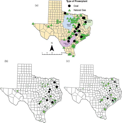
These transformations in fuel use for electricity generation also have impacts on emissions and air quality, but the overall impacts can be complex, as will be illustrated with two case studies from Texas. In the Texas electrical grid, operated by the Electricity Reliability Council of Texas (ERCOT), coal-based generation decreased from 37% of generation in 2008 to 24% in 2014 (ERCOT, 2009, 2015). In ERCOT, natural gas–fired units generally have lower air pollutant emissions per kilowatt hour of generation, relative to the coal plants, so when lower natural gas prices drive shifts from coal-based generation to natural gas–based generation, emissions of NO_x, particulate matter (PM), sulfur oxides (SO_x), and carbon dioxide decrease (Alhajeri et al., 2011). Pacsi et al. (2013, 2015) have modeled the electricity generation shifts, from coal to natural gas, that would be expected in ERCOT as natural gas prices change from $7.74 per million BTU (a representative price from 2006 to 2008), to $3.87 per million BTU, $2.88 per million BTU (an average price in late 2012) and $1.89 per million BTU (the price in late 2015, and a price equivalent to coal on an energy basis). Changes in emissions of NO_x, VOCs, CO, SO_x, and PM from these changes in electricity generation were estimated and compared with emissions due to added natural gas production in the Barnett Shale and Eagle Ford natural gas production regions that would be required to fuel the switch from coal to natural gas. As a result of these changes, emissions increase locally in the natural gas production areas as natural gas production increases; emissions decrease from the coal-fired power plants that are not utilized as extensively, but increase at natural gas–fired power plants that are used more extensively. Overall emissions throughout the ERCOT region decrease, but because the emission decreases and increases occur in different locations, the overall impact on air quality is complex. Figures 13 and 14 illustrate patterns of changes in ozone concentrations and electricity generation. As coal-fired power generation decreases, emission reductions are predicted to occur primarily at large coal-fired power plants in northeast Texas. The reduced NO_x emissions from these sources lead to significant reductions in ozone concentrations in northeast Texas and downwind regions, because the high emissions of biogenic hydrocarbons in the region create conditions that are conducive to ozone formation. Similarly, the emissions of NO_x from oil and natural gas production in the Eagle Ford lead to increased ozone concentrations in south Texas, as this region also has high emissions of biogenic hydrocarbons. In contrast, the emissions from oil and gas production in the Barnett Shale lead to small changes in ozone formation. Emissions of biogenic hydrocarbons in the region are low; other reactive hydrocarbons from the Dallas and Fort Worth metropolitan areas located close to or within the Barnett Shale have generally already reacted before they encounter the NO_x emissions from the oil and gas production activities, and the reactivity of the VOC emissions emitted by the oil and gas production activities is generally low.

Figure 13. (a) Decreases in summer month average daily maximum 8-hr ozone concentration due to shifting of electricity generation from coal- to natural gas–fired units, based on a natural gas price change from $7.74 per million BTU to $2.88 per million BTU; the shift from coal- to natural gas–fired generation lowers NO_x emissions, lowering ozone concentration. (b) Increases in summer month average daily maximum 8-hr ozone concentration due to increases in Eagle Ford production sufficient to supply the natural gas for the increased natural gas consumption in electricity generation.

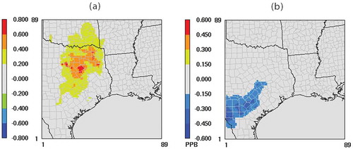
Figure 14. (a) Locations of coal-fired and natural gas–fired power generation, relative to oil and gas production regions in Texas; (b) distribution of electricity generation at high natural gas prices (sizes of dots representing power plants is proportional to extent of generation); (c) distribution of electricity generation at low natural gas prices (sizes of dots proportional to extent of generation) (Pacsi et al., 2013, 2015).

These contrasting case studies of the Barnett and Eagle Ford shales suggest that the full supply chain air quality impacts of natural gas production and electricity generation will be location dependent. In Texas, the switch from coal- to natural gas–fired electricity generation leads to relatively large air quality improvements in some areas because the emission reductions from coal-fired electricity generation occur in regions with conditions that are conducive to ozone formation. Ozone concentrations increase in some oil and gas production regions, but not others, because the reactivity of the hydrocarbons present in the atmosphere in the different production regions is very different.

Other complex changes in air quality, due to changes in patterns of utilization of the production from oil and natural gas fields, are possible. For example, increased availability of and low price of NGPLs are changing the feedstocks used in chemical manufacturing from petroleum products (naphthas) to NGPLs (DeRosa and Allen, 2015). This can also influence the magnitude and spatial and temporal patterns of emissions.

Emission management and control

A variety of voluntary and mandatory mitigation efforts at both state and federal levels have either occurred or are underway to reduce the emissions described in this review (Code of Federal Regulations [CFR], 2012). For methane emissions, the Natural Gas Star program (EPA 2015e) has resulted in the documentation of a number of approaches to reducing methane and VOC emissions. To cite just one example, for liquid unloadings (a source category that has been used as a case study multiple times in this review), advanced plunger lift control algorithms have been used to reduce venting (EPA, 2015f). Other mitigation strategies, based on experiences in the Natural Gas Star and other programs, have been summarized by the EPA in a series of white papers on emissions and mitigation strategies (EPA, 2015f). White papers for liquid unloadings, compressors, leaks, well completions, and pneumatic controllers are available. Many of these emission reduction strategies may be cost neutral, with the value of the recovered gas equaling or exceeding the cost of control. As shown in Table 8, ICF International, with support from Environmental Defense Fund, analyzed a variety of methane mitigation strategies for the natural gas supply chain and reported both the magnitude of the potential emission reductions and either the costs or the saving that could be achieved based on sale of recovered product (ICF International, 2014).

Table 8. Mitigation technologies for the natural gas supply chain with estimated magnitudes and costs/savings from implementing the method (ICF International, 2014)

Emission Reduction Method	Billions of Cubic Feet Of Methane Reduced	Cost Per Thousand Cubic Feet of Methane Reduced
Kimary pump to electric pump	5.8	($4.05)
Centrifugal compressor wet seal gas capture	19.1	($3.07)
Compressor station leak detection and repair	1.5	($3.03)
High bleed pneumatics—low bleed	25.4	($2.65)
Reciprocating compressors leak detection and repair	32.3	($0.33)
Condensate tank vapor control unit	0.4	$0.21
Stranded gas venting to flares	8.2	$0.30
Oil tank vapor control unit	5.5	$0.33
Pipeline venting to pump down	4.2	$0.53
Chemical injection pumps to solar pumps	4.8	$0.57
Uncontrolled liquid unloading to plunger lift	1.6	$0.74
Transmission station venting to gas capture	5.9	$1.27
Gathering/boosting leak detection and repair	3.3	$1.51
Intermittent bleed pneumatics to low bleed	12.1	$1.72
Oil well completion venting to flare	6.8	$2.13
Transmission compressor station leak detection and repair	2.8	$2.79
Well fugitives leak detection and repair	12.5	$3.51
Replace rod packing reciprocating compressors	3.6	$6.11
Meter and regulator leak detection and repair	7.1	$19.75
Total	162.9	$0.66

Notes: The middle column provides estimates of the magnitude of emission reductions possible; the right hand column gives an indication of the estimated cost per thousand cubic feet of gas emissions reduced.

Most of the approaches summarized in Table 8 involve replacement or repair of equipment. Changes in operating practices are also possible strategies for emission reduction. As just one example, for industrial process flares (a source category that has used as a case study multiple times in this review), training materials have been developed for operators of industrial flares that define practices for achieving both high combustion efficiencies and low smoke formation (University of Texas Center for Energy and Environmental Resources [UT CEER], 2016).

Finally, some mitigation approaches will require new technologies. For example, strategies for reducing the prevalence of super-emitters will rely on technologies for rapidly finding super-emitting sites and equipment. To address this need, the Advanced Research Projects Agency—Energy (ARPA-E) in 2015 launched the MONITOR program in which more than 10 teams of investigators are developing sensors or sensing systems capable of rapidly detecting and locating sources of methane emissions (ARPA-E, 2015). Other relatively new technologies include infrared cameras for sensing emissions and vehicle-mounted methane sensing for detecting high-emitting sites (Brandtley et al., 2015).

Summary and recommendations

National emission inventories indicate that VOC and NO_x emissions from oil and gas supply chains in the United States have been increasing significantly; however, national emission inventories for greenhouse gases have seen slight declines over the past decade. These emission inventory estimates are based on national scale counts of equipment and operational activities (activity factors), multiplied by average emission factors, and therefore these trends are subject to uncertainties in activity and emission factors. Although uncertainties associated with activity data and missing emission source types can be significant in some situations, multiple recent measurement studies indicate that the greatest uncertainties are associated with emission factors. In many source categories, small groups of devices or sites contribute a large fraction of emissions. Collectively, these sources have been referred to as “super-emitters.” When super-emitters are accounted for, multiple measurement approaches, at multiple scales, produce similar results for estimated emissions. Moving forward, it may be necessary to move away from single emission factors for source categories in the oil and gas supply chain (see eq 1) and to utilize separate emission factors (and activity counts) for super-emitters. Emission could then be estimated using the approach shown in eq 2:

(2)

where EF_i, _{super-emitter} is the emission factor for super-emitters in region I; EF_i, _{non-super-emitter} is the emission factor for non-super-emitters in region I; AF_i is activity factor for region I; f is the fraction of the activity factor attributed to super-emitters; and ER_i is the resulting emission rate total for region i.

Because super-emitters can be relatively small percentages of sources, accurately characterizing the fraction of super-emitters in the population (f) and the average emission rate for the super-emitters may necessitate large sampling programs to determine emission factors. Challenges moving forward will be understanding the causes of super-emitters and reducing their emission magnitudes. Work done to date suggests that both equipment malfunction and operational practices can be important. As improved emission estimates, accounting for super-emitters, are being developed, ongoing top-down measurement studies will continue to be important in evaluating the performance of existing inventories.

Other key information gaps include the limited information on air toxics emissions associated with oil and gas operations, and the limited amount of emission data available for oil and gas supply chains outside of the United States.

Finally, although most of this review has focused on emissions from energy supply infrastructures, the regional air quality implications of some coupled energy production and use scenarios have been examined. These case studies suggest that both energy production and use should be considered in assessing air quality implications of changes in energy infrastructures, and that impacts are likely to vary among regions.

Disclosure

David Allen has worked on research projects funded by a variety of governmental, nonprofit, and private sector sources, including the National Science Foundation, the U.S. Environmental Protection Agency, the Texas Commission on Environmental Quality, the American Petroleum Institute, and the Environmental Defense Fund. He has been a consultant for multiple organizations, including Eastern Research Group, RTI, and ExxonMobil, and he has served as Chair of EPA’s Science Advisory Board. Recently, he was the lead investigator for a study of methane emissions in natural gas production funded by the Environmental Defense Fund, Anadarko Petroleum Corporation, BG Group plc, Chevron, ConocoPhillips, Encana Oil & Gas (USA) Inc., Pioneer Natural Resources Company, SWEPI LP (Shell), Southwestern Energy, Statoil, Talisman Energy USA, and XTO Energy, an ExxonMobil subsidiary

Additional information

Notes on contributors

David T. Allen

Dr. David Allen is the Gertz Regents Professor of Chemical Engineering, and the Director of the Center for Energy and Environmental Resources, at the University of Texas at Austin. He is the author of seven books and over 200 papers, primarily in the areas of urban air quality, the engineering of sustainable systems, and the development of materials for environmental and engineering education. Dr. Allen has been a lead investigator for multiple air quality measurement studies, which have had a substantial impact on the direction of air quality policies. He has developed environmental educational materials for engineering curricula and for the university’s core curriculum, as well as engineering education materials for high school students. The quality of his work has been recognized with awards from the National Science Foundation, the AT&T Foundation, the American Institute of Chemical Engineers, the Association of Environmental Engineering and Science Professors, and the State of Texas. He has served on a variety of governmental advisory panels and from 2012 to 2015 chaired the U.S. Environmental Protection Agency’s Science Advisory Board. He has won teaching awards at the University of Texas and UCLA and the Lewis Award in Chemical Engineering Education, from the American Institute of Chemical Engineers.

Dr. Allen received his B.S. degree in chemical engineering, with distinction, from Cornell University in 1979. His M.S. and Ph.D. degrees in chemical engineering were awarded by the California Institute of Technology in 1981 and 1983. He has held visiting faculty appointments at the California Institute of Technology, the University of California, Santa Barbara, and the Department of Energy.

References

- Alamo Area Council of Governments (AACOG). 2013. Oil and Gas Emissions Inventory, Eagle Ford Shale, Technical Report. http://www.aacog.com/DocumentCenter/View/19069 (accessed January 2016).
- Alhajeri, N.S., P. Donohoo, A.S. Stillwell, C.W. King, M.D. Webster, M.E. Webber, and D.T. Allen. 2011. Using market-based dispatching with environmental price signals to reduce emissions and water use at power plants in the Texas grid. Environ. Res. Lett. 6:044018. doi:10.1088/1748-9326/6/4/044018
- Allen, D.T. 2014a. Atmospheric emissions and air quality impacts from natural gas production and use. Annu. Rev. Chem. Biomol. Eng. 5:55–75. doi:10.1146/annurev-chembioeng-060713-035938
- Allen, D.T. 2014b. Methane emissions from natural gas production and use: Reconciling bottom-up and top-down measurements. Curr. Opin. Chem. Eng. 5:78–83. doi:10.1016/j.coche.2014.05.004
- Allen, D.T., A. Pacsi, D. Sullivan, D. Zavala-Araiza, M. Harrison, K. Keen, M. Fraser, A.D. Hill, R.F. Sawyer, and J.H. Seinfeld. 2015a. Methane emissions from process equipment at natural gas production sites in the United States: Pneumatic controllers. Environ. Sci. Technol. 49:633–640. doi:10.1021/es5040156
- Allen, D.T., D. Sullivan, D. Zavala-Araiza, A. Pacsi, M. Harrison, K. Keen, M. Fraser, A.D. Hill, B.K. Lamb, R.F. Sawyer, and J.H. Seinfeld. 2015b. Methane emissions from process equipment at natural gas production sites in the United States: Liquid unloadings. Environ. Sci. Technol. 49:641–648, doi:10.1021/es504016r
- Allen, D.T., V.M. Torres, J. Thomas, D. Sullivan, M. Harrison, A. Hendler, S.C. Herndon, C.E. Kolb, M. Fraser, A.D. Hill, B.K. Lamb, J. Miskimins, R.F. Sawyer, and J.H. Seinfeld. 2013. Measurements of methane emissions at natural gas production sites in the United States. Proc. Natl. Acad. Sci. U. S. A. 110:17768–17773. doi:10.1073/pnas.1304880110
- Advanced Research Projects—Energy (ARPA-E). 2016. Methane Observation Networks with Innovative Technology to Obtain Reductions (MONITOR). http://arpa-e.energy.gov/?q=arpa-e-programs/monitor (accessed January 2016).
- Balcombe, P., K. Anderson, J. Speirs, N. Brandon, and A. Hawkes. 2015. Methane and CO2 Emissions from the Natural Gas Supply Chain: An Evidence Assessment. London: Sustainable Gas Institute, Imperial College. http://www.sustainablegasinstitute.org/publications/white-paper-1/ (accessed April 26, 2016).
- Brandt, A.R., G.A. Heath, E.A. Kort, F. O’Sullivan, G. Pétron, S.M. Jordaan, P. Tans, J. Wilcox, A.M. Gopstein, D. Arent, S. Wofsy, N.J. Brown, R. Bradley, G.D. Stucky, D. Eardley, and R. Harriss. 2014. Methane leaks from North American natural gas systems. Science 343:733–735. doi:10.1126/science.1247045
- Brantley, H.L., E.D. Thoma, W.C. Squier, B.B. Guven, and D. Lyon. 2015. Assessment of methane emissions from oil and gas production pads using mobile measurements. Environ. Sci. Technol. 49:7889−7895, doi:10.1021/es503070q
- Carter, W.P.L., and J. H. Seinfeld. 2012. Winter ozone formation and VOC incremental reactivities in the Upper Green River Basin of Wyoming. Atmos. Environ. 50:255–266. doi:10.1016/j.atmosenv.2011.12.025
- Caulton, D.R., P.B. Shepson, M.O. Cambaliza, D. McCabe, E. Baum, and B.H. Stirm. 2014a. Methane destruction efficiency of natural gas flares associated with shale formation wells. Environ. Sci. Technol. 48:9548–9554. doi:10.1021/es500511w
- Caulton, D.R., P.B. Shepson, R.L. Santoro, J.P. Sparks, R.W. Howarth, A.R. Ingraffea, M.O.L. Cambaliza, C. Sweeney, A. Karion, K.J. Davis, B.H. Stirm, S.A. Montzka, and B.R. Miller. 2014b. Toward a better understanding and quantification of methane emissions from shale gas development. Proc. Natl. Acad. Sci. U. S. A. 111:6237–6242. doi:10.1073/pnas.1316546111
- Code of Federal Regulations 40, Part 60 Subpart OOOO and NESHAP 40, CFR 63 Subpart HH, 77 FR 49490, Washington DC, August 16, 2012.
- Conley, S., G. Franco, I. Faloona, D.R. Blake, J. Peischl, and T.B. Ryerson. 2016. Methane emissions from the 2015 Aliso Canyon blowout in Los Angeles, CA. Science 351:1317–1320. doi:10.1126/science.aaf2348
- Daum, P., J. Meagher, D. Allen, and C. Durrenberger. 2002. Accelerated Science Evaluation of Ozone Formation in the Houston-Galveston Area: Summary. http://www.utexas.edu/research/ceer/texaqsarchive/pdfs/EXEC_SUMMARY_Nov_02.pdf (accessed January 2016).
- Daum, P.H., L.I. Kleinman, S.R. Springston, L.J. Nunnermacker, Y.N. Lee, J. Weinstein-Lloyd, J. Zheng, and C.M. Berkowitz. 2003. A comparative study of O3 formation in the Houston urban area and industrial plumes during the 2000 Texas Air Quality Study. J. Geophys. Res. 108(D23):4715. doi:10.1029/2003JD003552
- DeRosa, S., and D.T. Allen. 2015. Impact of natural gas and natural gas liquids supplies on the U.S. chemical manufacturing industry: Predicted cost and energy intensity effects and identification of bottleneck intermediates. ACS Sustain. Chem. Eng. 3:451–459. doi:10.1021/sc500236g
- Eastern Research Group and Sage Environmental. 2011. City of Fort Worth Natural Gas Air Quality Study, Final Report. http://fortworthtexas.gov/uploadedFiles/Gas_Wells/AirQualityStudy_final.pdf (accessed January 2016).
- Edwards, P.M., S.S. Brown, J.M. Roberts, R. Ahmadov, R.M. Banta, J.A. deGouw, W.P. Dubé, R.A. Field, J.H. Flynn, J.B. Gilman, M. Graus, D. Helmig, A. Koss, A.O. Langford, B.L. Lefer, B.M. Lerner, R. Li, S.-M. Li, S.A. McKeen, S.M. Murphy, D.D. Parrish, C.J. Senff, J. Soltis, J. Stutz, and C. Sweeney. 2014. High winter ozone pollution from carbonyl photolysis in an oil and gas basin. Nature 514:351–354. doi:10.1038/nature13767
- Electricity Reliability Council of Texas (ERCOT). 2009. ERCOT Quick Facts. http://www.ercot.com/content/news/presentations/2009/ERCOT%20Quick%20Facts%20May%202009.pdf (accessed January 2016).
- Electricity Reliability Council of Texas (ERCOT). 2015. ERCOT Quick Facts. http://www.ercot.com/content/news/presentations/2015/ERCOT_Quick_Facts_4315.pdf (accessed January 2016).
- Environmental Defense Fund (EDF). 2015. Aliso Canyon leak sheds light on national problem. https://www.edf.org/climate/aliso-canyon-leak-sheds-light-national-problem?utm_source=google&utm_campaign=ggad_aliso-canyon_upd_dmt&utm_medium=cpc&utm_id=1450803581&gclid=Cj0KEQiAq920BRC8-efn57XrotYBEiQAlVlMQ0EiaKhlErMTEFMMn5cVAM2nSHX7k9NxOmtiF5XStFUaAkit8P8HAQ (accessed January 2016).
- Gibbs, M. 2015. Improving Oil & Gas Emissions Tool Inputs Using Industry Surveys and Permit Data. Presentation to National Oil and Gas Emissions Committee, Oklahoma Department of Environmental Quality.
- Harrison, M.R., K.E. Galloway, A. Hendler, T.M. Shires, D. Allen, M. Foss, J. Thomas, and J. Spinhirne. 2011. Natural Gas Industry Methane Emission Factor Improvement Study, Final Report. Cooperative Agreement (with US EPA) XA-83376101. Austin, TX: University of Texas. http://www.utexas.edu/research/ceer/GHG/files/FReports/XA_83376101_Final_Report.pdf (accessed January 2016).
- Harrison, M.R., T.M. Shires, J.K. Wessels, and R.M. Cowgill. 1996. Methane Emissions from the Natural Gas Industry, Volumes 1–15, Final Report. GRI-94/0257 and EPA-600/R-96-080, Appendix B-1. Washington DC: Gas Research Institute and U.S. Environmental Protection Agency.
- Helmig, D., C.R. Thompson, J. Evans, P. Boylan, J. Hueber, and J.-H. Park. 2014. Highly elevated atmospheric levels of volatile organic compounds in the Uintah Basin, Utah. Environ. Sci. Technol. 48:4707−4715. doi:10.1021/es405046r
- Herndon, S.C., C. Floerchinger, J.R. Roscioli, T.I. Yacovitch, J.F. Franklin, J.H. Shorter, C.E. Kolb, R. Subramanian, A.L. Robinson, L.T. Molina, and D. Allen. 2013. Measuring methane emissions from industrial and waste processing sites using the dual tracer flux ratio method. Presented at the Annual Meeting the American Geophyscical Union, San Francisco, December 9–13, 2013.
- Herndon, S.C., J.T. Jayne, M.S. Zahniser, D.R. Worsnop, B. Knighton, E. Alwine, B.K. Lamb, M. Zavala, D.D. Nelson, J.B. McManus, J.H. Shorter, M.R. Canagaratna, T.B. Onasch, and C.E. Kolb. 2005. Characterization of urban pollutant emission fluxes and ambient concentration distributions using a mobile laboratory with rapid response instrumentation. Faraday Discuss. 130:327–339. doi:10.1039/b500411j
- ICF International. 2014. Economic Analysis of Methane Emission Reduction Opportunities in the U.S. Onshore Oil and Natural Gas Industries. Report to Environmental Defense Fund. https://www.edf.org/energy/icf-methane-cost-curve-report (accessed January 2016).
- Karion, A., C. Sweeney, E.A. Kort, J.B. Shepson, A. Brewer, M. Cambaliza, S.A. Conley, K. Davis, A. Deng, M. Hardesty, S.C. Herndon, T. Lauvaux, T. Lavoie, D. Lyon, T. Newberger, G. Pétron, C. Rella, M. Smith, S. Wolter, T.I. Yacovitch, and P. Tans. 2015. Aircraft-based estimate of total methane emissions from the Barnett Shale region. Environ. Sci. Technol. 49:8124–8131. doi:10.1021/acsest.5b00217
- Karion, A., C. Sweeney, G. Pétron, G. Frost, R.M. Hardesty, J. Kofler, B.R. Miller, T. Newberger, S. Wolter, R. Banta, A. Brewer, E. Dlugokencky, P. Lang, S.A. Montzka, R. Schnell, P. Tans, M. Trainer, R. Zamora, and S. Conley. 2013. Methane emissions estimate from airborne measurements over a western United States natural gas field. Geophys. Res. Lett. 40:1–5. doi:10.1002/grl.50811
- Kemball-Cook, S., A. Bar-Ilan, J. Grant, L. Parker, J. Jung, W. Santamaria, J. Matthews, and G. Yarwood. 2010. Ozone impacts of natural gas development in the Haynesville Shale. Environ. Sci. Technol. 44:9357–9363. doi:10.1021/es1021137
- Kimura, Y., G. McGaughey, M. Feldman, D.T. Allen, and E.C. McDonald-Buller. 2012. Spatial and temporal variability in OMI NO2 observations and NOx emissions inventories in Eastern Texas. Presented at the Air and Waste Management Association San Antonio, TX, June 19–22, 2012, Paper 2012-A-293- AWMA.
- Kolb, C.E., S.C. Herndon, J.B. McManus, J.H. Shorter, M.S. Zahniser, D.D. Nelson, J.T. Jayne, M.R. Canagaratna, and D.R. Worsnop. 2004. Mobile laboratory with rapid response instruments for real-time measurements of urban and regional trace gas and particulate distributions and emission source characteristics. Environ. Sci. Technol. 38:5694–5703. doi:10.1021/es030718p
- Kort, E.A., C. Frankenberg, K.R. Costigan, R. Lindenmaier, M.K. Dubey, and D. Wunch. 2014. Four corners: The largest US methane anomaly viewed from space. Geophys. Res. Lett. 41:6898–6903. doi:10.1002/2014GL061503
- Lamb, B.K., S.L. Edburg, T.W. Ferrara, T. Howard, M.R. Harrison, C.E. Kolb, A. Townsend-Small, W. Dyck, A. Possolo, and J.R. Whetstone. 2015. Direct measurements show decreasing methane emissions from natural gas local distribution systems in the United States. Environ. Sci. Technol. 49:5161−5169. doi:10.1021/es505116p
- Lamb, B.K., J.H. Shorter, J.B. McManus, C.E. Kolb, B.W. Mosher, R.C. Harriss, E. Allwine, D. Blaha, T. Howard, A. Guenther, R.A. Lott, R. Siverson, H. Westburg, and P. Zimmerman. 1995. Development of atmosphere tracer methods to measure methane emissions from natural gas facilities and urban areas. Environ. Sci. Technol. 29:1468–1478. doi:10.1021/es00006a007
- Laurenzi, I.J., and G.R. Jersey. 2013. Life Cycle greenhouse gas emissions and freshwater consumption of Marcellus Shale gas. Environ. Sci. Technol. 47:4896–4903. doi:10.1021/es305162w
- Litovitz, A., A. Curtright, S. Abramzon, N. Burger, and C. Samaras. 2013. Estimation of regional air quality damages from Marcellus Shale natural gas extraction in Pennsylvania. Environ. Res. Lett. 8:014017. doi:10.1088/1748-9326/8/1/014017
- Lyon, D.R., D. Zavala-Araiza, R.A. Alvarez, R. Harriss, V. Palacios, X. Lan, R. Talbot, T. Lavoie, P. Shepson, T.I. Yacovitch, S.C. Herndon, A.J. Marchese, D. Zimmerle, A.L. Robinson, and S.P. Hamburg. 2015. Constructing a spatially resolved methane emission inventory for the Barnett Shale region. Environ. Sci. Technol. 49:8147–8157. doi:10.1021/es506359c
- McKain, K., A. Down, S.M. Raciti, J. Budney, L.R. Hutyra, C. Floerchinger, S.C. Herndon, T. Nehrkorn, M.S. Zahniser, R.B. Jackson, N. Phillips, and S.C. Wofsy. 2015. Methane emissions from natural gas infrastructure and use in the urban region of Boston, Massachusetts. Proc. Natl. Acad. Sci. U. S. A. 112:1941–1946. doi:10.1073/pnas.1416261112
- McKenzie, L.M., R.Z. Witter, L.S. Newman, and J.L. Adgate. 2012. Human health risk assessment of air emissions from development of unconventional natural gas resources. Sci. Total Environ. 424:79–87. doi:10.1016/j.scitotenv.2012.02.018
- Medlock, K.B. 2012. Modeling the implications of expanded US shale gas production. Energy Strategy Rev. 1:33–41. doi:10.1016/j.esr.2011.12.002
- Miller, S.M., S.C. Wofsy, A.M. Michalak, E.A. Kort, A.E. Andrews, S.C. Biraud, E.J. Dlugokencky, J. Eluszkiewicz, M.L. Fischer, G. Janssens-Maenhout, B.R. Miller, J.B. Miller, S.A. Montzka, T. Nehrkorn, and C. Sweeney. 2013. Anthropogenic emissions of methane in the United States. Proc. Natl. Acad. Sci. U. S. A. 110:20018–20022. doi:10.1073/pnas.1314392110
- Mitchell, A.L., D.S. Tkacik, J.R. Roscioli, S.C. Herndon, T.I. Yacovitch, D.M. Martinez, T.L. Vaughn, L.L. Williams, M.R. Sullivan, C. Floerchinger, M. Omara, R. Subramanian, D. Zimmerle, A.J. Marchese, and A.L. Robinson. 2015. Measurements of methane emissions from natural gas gathering facilities and processing plants: Measurement results. Environ. Sci. Technol. 49:3219−3227. doi:10.1021/es5052809
- Murphy, C.F., and D.T. Allen. 2005. Hydrocarbon emissions from industrial release events in the Houston-Galveston area and their impact on ozone formation. Atmos. Environ. 39:3785–3798. doi:10.1016/j.atmosenv.2005.02.051
- National Research Council. 2001. Evaluating Vehicle Inspection and Maintenance Programs. Washington, DC: National Academies Press.
- Nicot, J., and B.R. Scanlon. 2012. Water use for shale-gas production in Texas. Environ. Sci. Technol. 46:3580–3586. doi:10.1021/es204602t
- Olaguer, E.P. 2012. The potential near-source ozone impacts of upstream oil and gas industry emissions. J. Air Waste Manage. Assoc. 62:966–977. doi:10.1080/10962247.2012.688923
- Oltmans, S., R. Schnell, B. Johnson, G. Pétron, T. Mefford, and R. Neely III. 2014. Anatomy of wintertime ozone associated with oil and natural gas extraction activity in Wyoming and Utah. Elem. Sci. Anthol. 2:000024. doi:10.12952/journal.elementa.000024
- Osborn, S.G., A. Vengosh, N.R. Warner, and R.B. Jackson. 2011. Methane contamination of drinking water accompanying gas-well drilling and hydraulic fracturing. Proc. Natl. Acad. Sci. U. S. A. 108: 8172–8176. doi:10.1073/pnas.1100682108
- Pacsi, A.P., N.S. Alhajeri, D. Zavala-Araiza, M.D. Webster, and D.T. Allen. 2013. Regional air quality impacts of increased natural gas production and use in Texas. Environ. Sci. Technol. 47:3521–3527. doi:10.1021/es3044714
- Pacsi, A.P., Y. Kimura, G. McGaughey, E.C. McDonald-Buller, and D.T. Allen. 2015. Regional ozone impacts of increased natural gas use in the Texas power sector and development in the Eagle Ford shale. Environ. Sci. Technol. 49:3966–3973. doi:10.1021/es5055012
- Pacsi, A.P., and M. Harrison. 2015. Emissions from liquid unloadings vary by region, UOGR, 3 (1). http://www.ogj.com/articles/uogr/print/volume-3/issue-1/emissions-from-liquid-unloadings-vary-by-region.html (accessed January 2016).
- Pavlovic, R.T., D.T. Allen, and E.C. McDonald-Buller. 2012. Temporal variability in flaring emissions in the Houston-Galveston area. Ind. Eng. Chem. Res. 51:12653–12662. doi:10.1021/ie2013357
- Peischl, J., T.B. Ryerson, K.C. Aikin, J.A. de Gouw, J.P. Gilman, J.S. Holloway, B.M. Lerner, R. Nadkarni, J.A. Neuman, J.B. Nowak, M. Trainer, C. Warneke, and D.D. Parrish. 2015. Quantifying atmospheric methane emissions from the Haynesville, Fayetteville, and northeastern Marcellus shale gas production regions. J. Geophys. Res. Atmos. doi:10.1002/2014JD022697
- Peischl, J., T.B. Ryerson, J. Brioude, K.C. Aikin, A.E. Andrews, E. Atlas, D. Blake, B.C. Daube, J.A. de Gouw, E. Dlugokencky, G.J. Frost, D.R. Gentner, J.B. Gilman, A.H. Goldstein, R.A. Harley, J.S. Holloway, J. Kofler, W.C. Kuster, P.M. Lang, P.C. Novelli, G.W. Santoni, M. Trainer, S.C. Wofsy, and D.D. Parrish. 2013. Quantifying sources of methane using light alkanes in the Los Angeles Basin, California. J. Geophys. Res. Atmos. 118:4974–4990. doi:10.1002/jgrd.50413
- Pétron, G., G. Frost G, B.R. Miller, A.I. Hirsch, S.A. Montzka, A. Karion, M. Trainer, C. Sweeney, A.E. Andrews, L. Miller, J. Kofler, A. Bar-Ilan, E.J. Dlugokencky, L. Patrick, C.T. Moore Jr., T.B. Ryerson, C. Sisco, W. Kolodzey, P.M. Lang, T. Conway, P. Novelli, K. Masarie, B. Hall, D. Guenther, D. Kitzis, J. Miller, D. Welsh, D. Wole, W. Neff, and P. Tans. 2012. Hydrocarbon emissions characterization in the Colorado front range: A pilot study. J. Geophys. Res. 117(D4): D04304. doi:10.1029/2011JD016360
- Pétron, G., A. Karion, C. Sweeney, B.R. Miller, S.A. Montzka, G.J. Frost, M. Trainer, P. Tans, A. Andrews, J. Kofler, D. Helmig, D. Guenther, E. Dlugokencky, P. Lang, T. Newberger, S. Wolter, B. Hall, P. Novelli, A. Brewer, S. Conley, M. Hardesty, R. Banta, A. White, D. Noone, D. Wolfe, and R. Schnell. 2014. A new look at methane and nonmethane hydrocarbon emissions from oil and natural gas operations in the Colorado Denver-Julesburg Basin. J. Geophys. Res. Atmos. 119:6836–6852. doi:10.1002/2013JD021272
- Prasino Group. 2013. Final Report for Determining Bleed Rates for Pneumatic Devices in British Columbia. Report to British Columbia Ministry of Environment.
- Rahm, B., and S. Riha. 2012. Toward strategic management of shale gas development: Regional, collective impacts on water resources. Environ. Sci. Policy 17:12–23. doi:10.1016/j.envsci.2011.12.004
- Rich, A., J.P. Grover, and M.L. Sattler. 2014. An exploratory study of air emissions associated with shale gas development and production in the Barnett Shale. J. Air Waste Manage. Assoc. 64:61–72. doi:10.1080/10962247.2013.832713
- Ryerson, T.B., M. Trainer, W.M. Angevine, C.A. Brock, R.W. Dissly, F.C. Fehsenfeld, G.J. Frost, P.D. Goldan, J.S. Holloway, G. Hubler, R.O. Jakoubek, W.C. Kuster, J.A. Neuman, D.K. Nicks Jr., D.D. Parrish, J.M. Roberts, and D.T. Sueper, E.L. Atlas, S.G. Donnelly, F. Flocke, A. Fried, W.T. Potter, S. Schauffler, V. Stroud, A.J. Weinheimer, B.P. Wert, and C. Wiedinmyer, R.J. Alvarez, R.M. Banta, L.S. Darby, and C.J. Senff. 2003. Effect of petrochemical industrial emissions of reactive alkenes and NOx on tropospheric ozone formation in Houston, Texas. J. Geophys. Res. 108(D8):4249. doi:10.1029/2002JD003070
- Schnell, R.C., S.J. Oltmans, R.R. Neely, M.S. Endres, J.V. Molenar, and A.B. White. 2009. Rapid photochemical production of ozone at high concentrations in a rural site during winter. Nat. Geosci. 2:120–122. doi:10.1038/NGEO415
- Smith, M.L., E.A. Kort, A. Karion, C. Sweeney, S.C. Herndon, and T.I. Yacovitch. 2015. Airborne ethane observations in the barnett shale: Quantification of ethane flux and attribution of methane emissions. Environ. Sci. Technol. 49:8158–8166. doi:10.1021/acsest.5b00219
- Shorter, J.H., J.B. McManus, C.E. Kolb, E.J. Allwine, R. Siverson, B.K. Lamb, B.W. Mosher, R.C. Harriss, T. Howard, and R.A. Lott. 1997. Collection of leakage statistics in the natural gas system by tracer methods. Environ. Sci. Technol. 31:2012–2019. doi:10.1021/es9608095
- Stedman, D.H. 1989. Automobile carbon monoxide emission. Environ. Sci. Technol. 23:147–149. doi:10.1021/es00179a002
- Streets, D.G., G.R. Carmichael, B. de Foy, R.R. Dickerson, B.N. Duncan, D.P. Edwards, J.A. Haynes, D.K. Henze, M.R. Houyoux, D.J. Jacob, N.A. Krotkov, L.N. Lamsal, Y. Liu, Z. Lu, R.V. Martin, G.G. Pfister, R.W. Pinder, and K.J. Wecht. 2013. Emissions estimation from satellite retrievals: A review of current capability. Atmos. Environ. 77:1011–1042. doi:10.1016/j.atmosenv.2013.05.051
- Subramanian, R., L.L. Williams, T.L. Vaughn, D. Zimmerle, J.R. Roscioli, S.C. Herndon, T.I. Yacovitch, C. Floerchinger, D.S. Tkacik, A.L. Mitchell, M.R. Sullivan, T.R. Dallmann, and A.L. Robinson. 2015. Methane emissions from natural gas compressor stations in the transmission and storage sector: Measurements and comparisons with the EPA Greenhouse Gas Reporting Program Protocol. Environ. Sci. Technol. 49:3252−3261 doi:10.1021/es5060258
- Tang, W., D. Cohan, L.N. Lamsal, X. Xiao, and W. Zhou. 2013. Inverse modeling of Texas NOx emissions using space-based and ground-based NO2 observations. Atmos. Chem. Phys. 13:11005–11018. doi:10.5194/acp-13-11005-2013
- Tang, W., D. Cohan, A. Pour-Biazar, L.N. Lamsal, A. White, X. Xiao, W. Zhou, B.H. Henderson, and B.F. Lash. 2014. Influence of satellite-derived photolysis rates and NOx emissions on Texas ozone modeling. Atmos. Chem. Phys. 14:24475–24522. doi:10.5194/acpd-15-1601-2015
- Townsend-Small, A., J.E. Marrero, D.R. Lyon, I.J. Simpson, S. Meinardi, and D.R. Blake. 2015. Integrating source apportionment tracers into bottom-up inventory of methane emissions in the Barnett Shale hydraulic fracturing region. Environ. Sci. Technol. 49:8175–8182. doi:10.1021/acsest.5b00057
- Texas Commission on Environmental Quality. 2012. Barnett Shale Geological Area. Austin, TX: Texas Commission on Environmental Quality. http://www.tceq.texas.gov/airquality/barnettshale (accessed January 2016).
- Texas Commission on Environmental Quality. 2015a. Emission Event Report Database. http://www2.tceq.texas.gov/oce/eer/ (accessed January 2016).
- Texas Commission on Environmental Quality. 2015b. Data collected by Automated Gas Chromatographs (AutoGCs). https://www.tceq.texas.gov/airquality/monops/agc/autogc.html (accessed January 2016).
- Texas Commission on Environmental Quality. 2015c. Automated Gas Chromatographs (AutoGCs). Barnett Shale Monitoring Network. https://www.tceq.texas.gov/airquality/monops/agc/agc_barnett.html (accessed January 2016).
- Texas Railroad Commission 2015. Texas Barnett Shale Total Natural Gas Production 2000 through October 2015. http://www.rrc.state.tx.us/media/22204/barnettshale_totalnaturalgas_day.pdf (accessed January 2016).
- Torres, V.M., S. Herndon, and D.T. Allen. 2012a. Industrial flare performance at low flow conditions: Part 2. Air and steam assisted flares. Ind. Eng. Chem. Res. 51:12569–12576. doi:10.1021/ie202675f
- Torres, V.M., S. Herndon, Z. Kodesh, and D.T. Allen. 2012b. Industrial flare performance at low flow conditions: Part 1. Study overview. Ind. Eng. Chem. Res. 51:12559–12568. doi:10.1021/ie202674t
- U.S. Energy Information Administration. 2015a. International Energy Statistics, 2014. Washington, DC: U.S. Department of Energy. http://www.eia.gov/beta/international/ (accessed January 2016).
- U.S. Energy Information Administration. 2015b. Petroleum, 2015. Washington, DC: U.S. Department of Energy. http://www.eia.gov/petroleum/ (accessed January 2016).
- U.S. Energy Information Administration. 2015c. Natural Gas, 2015. EPA 430-R-14-003. Washington, DC: U.S. Department of Energy. http://www.eia.gov/naturalgas/ (accessed January 2016).
- U.S. Energy Information Administration. 2015d. Monthly Energy Review, December 2015. Washington, DC: U.S. Department of Energy. http://www.eia.gov/totalenergy/data/monthly/ (accessed January 2016).
- U.S. Energy Information Administration. 2015e. Electricity 2015. Washington, DC: U.S. Department of Energy. http://www.eia.gov/electricity/ (accessed January 2016).
- U.S. Energy Information Administration. 2015f. Annual Energy Outlook 2015. Washington, DC: U.S. Department of Energy. http://www.eia.gov/forecasts/aeo/ (accessed January 2016).
- U.S. Energy Information Administration. 2015g. Natural Gas Processing Plants in the United States: 2010 Update. Washington, DC: U.S. Department of Energy. http://www.eia.gov/pub/oil_gas/natural_gas/feature_articles/2010/ngpps2009/ (accessed January 2016).
- U.S. Energy Information Administration. 2015h. Eagle Ford Region, Drilling Productivity Report, December 2015. Washington, DC: U.S. Department of Energy. https://www.eia.gov/petroleum/drilling/pdf/eagleford.pdf (accessed January 2016).
- U.S. Environmental Protection Agency. 2009. Section 812 Prospective Study of the Benefits and Costs of the Clean Air Act: Air Toxics Case Study—Health Benefits of Benzene Reductions in Houston, 1990–2020. Report to U.S. Environmental Protection Agency, July 14, 2009. http://www.epa.gov/sites/production/files/2015-07/documents/812caaa_benzene_houston_final_report_july_2009.pdf (accessed January 2016).
- U.S. Environmental Protection Agency. 2012. Study of the Potential Impacts of Hydraulic Fracturing on Drinking Water Resources. EPA 601/R-12/011. Washington, DC: U.S. Environmental Protection Agency.
- U.S. Environmental Protection Agency. 2015a, National Emission Inventory, 2011, version 2. http://www.epa.gov/air-emissions-inventories/national-emissions-inventory (accessed January 2016).
- U.S. Environmental Protection Agency. 2015b. Greenhouse Gas Reporting Program. http://ghgdata.epa.gov/ghgp/ (accessed November 2015).
- U.S. Environmental Protection Agency. 2015c. Inventory of U.S. Greenhouse Gas Emissions and Sinks: 1990–2013.
- U.S. Environmental Protection Agency. 2015d. Greenhouse Gas Reporting Program. 2011-2012-2013 GHGRP Industrial Profiles Petroleum and Natural Gas Systems. http://www2.epa.gov/sites/production/files/2015-10/documents/subpart_w_2014_data_summary_10-05-2015_final.pdf (accessed December 2015).
- U.S. Environmental Protection Agency. 2015e. Natural Gas STAR. http://www3.epa.gov/gasstar/index.html (accessed January 2016).
- U.S. Environmental Protection Agency. 2015f. Methane: Addressing greenhouse gases and smog forming VOCs from the oil and gas industry. http://www3.epa.gov/airquality/oilandgas/methane.html (accessed January 2016).
- University of Texas Bureau of Economic Geology (UT BEG). 2013. Press Release: New, Rigorous Assessment of Shale Gas Reserves Forecasts Reliable Supply from Barnett Shale through 2030, February 28, 2013. Austin, TX: University of Texas http://www.utexas.edu/news/2013/02/28/new-rigorous-assessment-of-shale-gas-reserves-forecasts-reliable-supply-from-barnett-shale-through-2030/ (accessed January 2016).
- University of Texas Center for Energy and Environmental Resources (CEER). 2016. Supplemental Flare Operations Training for Plant Personnel. https://sfot.ceer.utexas.edu/ (accessed January 2016).
- Vidic, R.D., S.L. Brantley, J.M. Vandenbossche, D. Yoxtheimer, and J.D. Abad. 2013. Impact of shale gas development on regional water quality. Science 340:1235009. doi:10.1126/science.1235009
- Vizuete, W., Y. Kimura, H. Jeffries, and D.T. Allen. 2008. Modeling ozone formation from industrial emission events in Houston, Texas. Atmos. Environ. 42:7641–7650. doi:10.1016/j.atmosenv.2008.05.063
- Webster, M., J. Nam, Y. Kimura, H. Jeffries, W. Vizuete, and D.T. Allen. 2007. The effect of variability in industrial emissions on ozone formation in Houston, Texas. Atmos. Environ. 41:9580–9593. doi:10.1016/j.atmosenv.2007.08.052
- Wennberg, P.O., W. Mui, D. Wunch, E.A. Kort, D.R. Blake, E.L. Atlas, G.W. Santoni, S.C. Wofsy, G.S. Diskin, S. Jeong, and M.C. Fischer. 2012. On the sources of methane to the Los Angeles atmosphere. Environ. Sci. Technol. 46:9282–9289. doi:10.1021/es301138y
- Zavala-Araiza, D. 2014. Atmospheric Emissions and Air Quality Impacts of Natural Gas Production from Shale Formations. Ph.D. dissertation, University of Texas at Austin, Austin, Texas.
- Zavala-Araiza, D., D.T. Allen, M. Harrison, F.C. George, and G.R. Jersey. 2015a. Allocating Methane emissions to natural gas and oil production from shale formations. ACS Sustain. Chem. Eng. 3:492–498. doi:10.1021/sc500730x
- Zavala-Araiza, D., D. Lyon, R.A. Alvarez, V. Palacios, R. Harriss, X. Lan, R. Talbot, and S.P. Hamburg. 2015b. Toward a functional definition of methane super-emitters: Application to natural gas production sites. Environ. Sci. Technol. 49:8167−8174, doi:10.1021/acs.est.5b00133
- Zavala-Araiza, D., D.R. Lyon, R.A. Alvarez, K.J. Davis, R. Harriss, S.C. Herndon, A. Karion, E.A. Kort, B.K. Lamb, X. Lan, A.J. Marchese, S.W. Pacala, A.L. Robinson, P.B. Shepson, C. Sweeney, R. Talbot, A. Townsend-Small, T.I. Yacovitch, D.J. Zimmerle, and S.P. Hamburg. 2015c. Reconciling divergent estimates of oil and gas methane emissions. Proc. Natl. Acad. Sci. U. S. A. 112:15597–15602. doi:10.1073/pnas.1522126112
- Zavala-Araiza, D., D.W. Sullivan, and D.T. Allen. 2014. Atmospheric hydrocarbon emissions and concentrations in the Barnett Shale natural gas production region. Environ. Sci. Technol. 48:5314–5321. doi:10.1021/es405770h
- Zimmerle, D., A.J. Marchese, and A.L. Robinson. 2015. Measurements of methane emissions from natural gas gathering facilities and processing plants: Measurement results. Environ. Sci. Technol. 49:3219−3227. doi:10.1021/es5052809