A comparison of correlation-length estimation methods for the objective analysis of surface pollutants at Environment and Climate Change Canada

ABSTRACT

An objective analysis is one of the main components of data assimilation. By combining observations with the output of a predictive model we combine the best features of each source of information: the complete spatial and temporal coverage provided by models, with a close representation of the truth provided by observations. The process of combining observations with a model output is called an analysis. To produce an analysis requires the knowledge of observation and model errors, as well as its spatial correlation. This paper is devoted to the development of methods of estimation of these error variances and the characteristic length-scale of the model error correlation for its operational use in the Canadian objective analysis system. We first argue in favor of using compact support correlation functions, and then introduce three estimation methods: the Hollingsworth–Lönnberg (HL) method in local and global form, the maximum likelihood method (ML), and the diagnostic method. We perform one-dimensional (1D) simulation studies where the error variance and true correlation length are known, and perform an estimation of both error variances and correlation length where both are non-uniform. We show that a local version of the HL method can capture accurately the error variances and correlation length at each observation site, provided that spatial variability is not too strong. However, the operational objective analysis requires only a single and globally valid correlation length. We examine whether any statistics of the local HL correlation lengths could be a useful estimate, or whether other global estimation methods such as by the global HL, ML, or should be used. We found in both 1D simulation and using real data that the ML method is able to capture physically significant aspects of the correlation length, while most other estimates give unphysical and larger length-scale values.

Implications: This paper describes a proposed improvement of the objective analysis of surface pollutants at Environment and Climate Change Canada (formerly known as Environment Canada). Objective analyses are essentially surface maps of air pollutants that are obtained by combining observations with an air quality model output, and are thought to provide a complete and more accurate representation of the air quality. The highlight of this study is an analysis of methods to estimate the model (or background) error correlation length-scale. The error statistics are an important and critical component to the analysis scheme.

Introduction

Objective analyses of surface pollutants are essentially surface maps of air pollutants that are obtained by combining surface observations with an air quality model output. Because observations are close to the truth and model outputs provide a complete spatial and temporal coverage, their combination in the form of objective analyses is thought to provide a more accurate and complete representation of the surface air quality. These maps are called “analyses.” The term “objective” has, however, a historical origin, meaning that these maps are produced objectively using an estimation method rather than by hand by a meteorologist or an air quality expert, which would then be a subjective analysis. Also refer to Table 1, for explanation of some of the terms used in data assimilation.

Table 1. Terminology of data assimilation.

Terminology	Explanation
Analysis	Best representation of air quality over an area, resulting from combining all available observations with an air quality model (called the prior). The analysis is sometime called the posterior.
Objective analysis	The term “objective” has an historical origin; it is simply a reminder that the analysis is produced objectively using an estimation method or algorithm rather than by hand by a meteorologist or an air quality expert, which would then be called a subjective analysis.
Data assimilation	A cycle of analyses and forecasts that runs over time. Data assimilation effectively accumulates observation information from the past up to the current time, and thus provides a more accurate depiction of the state of the atmosphere. It is different from a single analysis that provides basically a snapshot at a given time.
Data fusion	The combination of observations and information from different sources and proxies, such as land use, population density, proximity of major roads, etc., to produce a better depiction of the atmospheric state. This is done typically by using statistical methods and graphical information systems (GIS). However, it does not use a predictive air quality model, nor does it use the “analysis” to initialize an air quality model, and thus should not be confused with data assimilation.
Correlation length	The distance by which the correlation function reaches a given a prescribed value (here set at 0.606). The correlation function represents the influence function in space of a correction due to a single point observation. The prescribed value is somewhat arbitrary, but in data assimilation it is becoming common to use the correlation value of a Gaussian correlation function for a (dimensionless) length-scale parameter value equal to 1.
Correlation length-scale parameter	The value of a length-scale parameter that appears in a particular correlation function. It is not equal to the decorrelation length that the particular correlation function will display. Sometimes the terminology correlation length and correlation length-scale parameter are used interchangeably, but this creates confusion.
Spatially homogeneous correlation	A spatial correlation pattern (usually horizontal) that does not change when evaluated with respect to a different reference point. Mathematically, it means that the correlation is invariant under translation of the coordinates, that is, .
Spatially isotropic correlation	A spatial correlation pattern (usually horizontal) that is identical in any direction from a reference point. Mathematically, it means a correlation that is invariant under any rotation of the coordinate system.
Gaussian correlation model	Basically a spatial correlation model whose dependence on distance r has the form . It is also known as the squared-exponential model, and should not be confused with a Gaussian probability function
Innovations	This is a term that comes from that Kalman filter theory and means the portion of the observation signal that is not already explained by the prior. In data assimilation we refer it to the observed-minus-model (or forecast) residuals.
Observation space	The ensemble of location of the observations and the physical quantities being measured that are used to form an analysis. In contrast with the model space that is generally a gridded space of the model grid points, the observation space is nonuniform and heterogeneous, and has its own characteristics for each observation types (e.g., Airnow surface observation network, satellite derived AOD, etc.).
Background	Means the state of a prognostic air quality model at a given time. In data assimilation it is the prior over which observations are combined to yield an analysis.
Kalman filter	A data assimilation method that propagates and updates its state estimate and associated error covariance over time and as it processes observations. The observations will in general reduce the uncertainties while the model may increase it over time due to a model error growth. In data assimilation the Kalman filter is prohibitive, and alternative formulations such as ensemble based formulation have been developed. For chemical data, assimilation sequential filters are another computationally efficient alternative.
Sequential filter	A simplified Kalman filter where only error variances are evolved by transport and updated by observations. It is a scheme used principally in chemical data assimilation.
3D Var, 4D Var	Methods to produce an analysis using a variational approach, and that are performed numerically by minimizing some cost function. 3D Var means that the analysis is obtained in the three-dimensional physical space. 4D Var uses the prognostic model to produce a spatial and temporal analysis, given all observations available in a time window.

There are many potential applications for objective analyses. Over extended time periods, the surface objective analyses are useful to assess long-term effect of air quality on human health (e.g., Crouze et al., 2015; Lee and Liu, 2014). If three-dimensional analyses are produced, they can be used to initialize air quality forecast model, a process known as data assimilation which can improve in air quality forecasts (e.g., Elbern et al., 2007; Wu et al., 2008).

To produce objective analyses, we generally use a Bayesian framework where it is assumed that the observation likelihood and model, called the prior, are Gaussian distributed. The observation errors are typically spatially uncorrelated (or their spatial correlations can be neglected) while the model prior probability distribution exhibits significant spatial correlations on distances resolved by the air quality model. These facts are supported by a vast number of data assimilation studies. To perform an analysis we thus need to know the observation error variance at each observation sites, the model error variances distributed in space, and the spatial correlation structure of the model prior.

A range of methods have been proposed for air quality data assimilation such as: optimum interpolation, 3D Var, 4D Var, the sequential filter, and the ensemble Kalman filter (for reviews see Sandu et al., 2011; Bocquet et al., 2015). The ensemble Kalman filter and 4D Var use the model itself to produce terrain- and flow-dependent spatial correlation structures. Although they may be considered realistic, they require several model integrations over a given time period to produce flow-dependent correlation structures and are thus computationally prohibitive, considering computing resources needed for air quality forecast models. For real-time operational use, simpler methods such as optimum interpolation or 3D Var are preferred.

In optimum interpolation or 3D Var the spatial correlation structure of the model prior is assumed to be homogeneous and isotropic, which means that the correlation function with respect to a reference point is the same for any reference point (i.e., is invariant under translation), and the correlation is the same in any direction (i.e., is invariant under rotation). These assumptions are introduced to simplify the characterization of correlation functions, thus reducing them to a correlation model type and a correlation length (i.e., the length by which the correlation value decreased by a certain fixed value—see “Correlation Length Estimation Methods” section). In optimum interpolation, we use past data of observation-minus-model residuals to estimate the correlation length, and determine by inspection which correlation model type best fits the data. Indeed, if we consider that an observation is a measurement of the truth plus an observation error, and that a model is also a representation of the truth plus a model error, then the observation-minus-model residuals are simply a combination of observation and model errors. Furthermore, and as we said earlier, the observation errors are generally spatially uncorrelated, while model errors exhibit a significant spatial correlation. If in addition we assume (as it is sometimes verified) that the observation and model errors are uncorrelated, then the spatial autocorrelation function of the observed-minus-model residuals display a spatially correlated component and a spatially uncorrelated component. The spatially correlated component is attributed to the model prior, while the spatially uncorrelated component is attributed to the observation error. Observed-minus-model residuals are also known in data assimilation as “innovation,” which means “the portion of the observation signal that is not already explained by the model.”

In this paper we are not using analyses to initialize the model forecasts. The analyses are created “off-line” of a data assimilation cycle and are used for air quality monitoring purposes only. In this study we first validate the estimation of nonuniform error variances (at each observation site) and then we focus on estimating the model prior correlation length (also called the “background error correlation length” in data assimilation). To estimate the correlation length or its spectra, several methods have been developed, such as: the National Meteorological Center (NMC) lagged-forecast method (Parrish and Derber, 1992), the ensemble of data assimilation (EDA) method (Fisher, 2003), the Hollingsworth–Lönnberg (1986) (HL) method, the diagnostic method (Ménard and Chang, 2000; Ménard et al., 2000), and the maximum likelihood method (Dee and da Silva, 1999a, 1999b). The NMC method and the EDA methods require cycles of analysis forecasts and are thus not applicable to off-line analyses. Another very popular method developed by Desroziers et al. (2005) uses analysis increments (i.e., the difference between the analysis and the model prior) to estimate error variances rather than error correlations and is not considered here. We thus concentrate our comparison between the Hollingsworth–Lönnberg, the diagnostic and the maximum likelihood methods.

• The Hollingsworth–Lönnberg method (HL) was originally developed for the optimum interpolation method by Rutherford (1972) and refined by Hollingsworth and Lönnberg (1988). It estimates the correlation length and the ratio of observation to model error variances by a least-square fit of a correlation model against the sample of the spatial autocorrelation of observation-minus-model residuals.

• The diagnostic is a diagnostic of fit between the innovations and the sum of observation and background error covariances in observation space (Talagrand, 1998; Ménard, 2000). The method was applied to Kalman filter chemical data assimilation by Ménard and Chang (2000) to estimate observation and model error variance growth rate. In other contexts where the model error variance is known or computed, such as with the sequential filter (i.e., a simplified version of the Kalman filter that evolves only error variances), the diagnostic can then be used to determine the correlation length (Rösevall et al., 2007).

• The maximum likelihood estimation is a well-established estimation method of parameters of a statistical model, and is used when no prior information is available. It has been used in the context of data assimilation to estimate error covariance parameters by Dee and daSilva (1999a, 1999b). This approach has also been applied to estimate the model error in ensemble Kalman filters (e.g., Mitchell and Houtekamer, 2000) and to estimate the cross observation–background error correlation (e.g., Tangborn et al., 2002), but we know of no studies that use this method in the context of chemical data assimilation.

In the literature of air quality data assimilation, widely ranging estimated correlation lengths have been obtained. For example, in the case of O₃ in late afternoon summer, correlation length of about 250 km were obtained with regional data assimilation over Europe (Wu et al., 2008; Frydendall et al., 2009) and over North America (Chai et al., 2007) using the HL method, while Pagowski et al. (2010) obtained values of the order of 125 km using the NMC method. Data assimilation over smaller areas and denser observation networks over Germany and Belgium reported smaller correlation lengths of the order of 60 km (Elbern and Schmidt, 2001; Tilmes, 2001; Hoelzemann et al., 2001; Elbern et al., 2007; Kumar et al., 2012), with similar length for PM₁₀ (Tombette et al., 2009). Even shorter correlation lengths were reported by Sillibelo et al. (2014) when assimilating over central Italy and Rome domain (~25 km, ~10 km, respectively). These discrepancies arise because, in a data assimilation system, the model error statistics are not independent of the observing network. Indeed, because the observation errors are spatially uncorrelated, the analysis error correlation length is smaller than the prior correlation length. In the forecast step, the model uses the analysis as an initial condition. The short-term forecast creates changes in error variances and correlation length but still has some memory of the analysis error covariance used as an initial condition. The short-term forecast is then the prior for the next batch of observations. Overall, in the data assimilation cycle, the model error correlation is thus not independent of the observation network. If the observations have more weight, or if the observation network has higher density, the resulting correlation length of the prior in an assimilation cycle is shorter (e.g., Daley and Ménard, 1993; Bannister, 2008, section 6.5). Furthermore, if the NMC method is used to provide an estimation of the correlation length, it is important to note that the NMC method does not in fact estimate the background error correlation but rather the impact an observation network has on reducing the error variances and error correlation length on the prior, as pointed out by Bouttier (1994) and Bannister (2008). Thus, the NMC method provides smaller correlation length than those obtained by the HL method. Overall, in comparing correlation lengths obtained from different studies, it is important to keep in mind that these estimates are dependent on the observations and that some methods may provide different estimates.

However, we wish to emphasize that in this study, the correlation lengths obtained are for off-line analyses. The correlation length estimates are not influenced by the observation network and are rather a characteristic of the air quality model itself. Furthermore, our correlation length estimates are expected to be somewhat larger than those derived in a data assimilation cycle.

The paper is organized as follows. We first give an overview of the current operational implementation of the objective analysis at Environment and Climate Change Canada (ECCC, formerly known as Environment Canada) and then present arguments in favor of using compact support correlation functions. Next, we give a description of the methods used to estimate the error statistics, and examine the results first in a simulated environment where we know the true errors statistics. Then we apply those techniques to the objective analysis that uses the Airnow observations and the Canadian air quality model GEM-MACH (Moran et al., 2014) as prior. Finally, we give a short summary and some conclusions.

Background on the operational objective analysis at ECCC

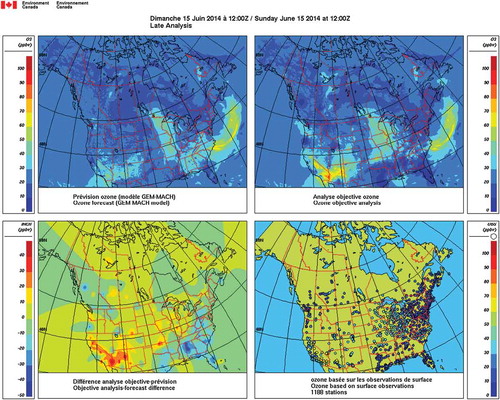
In February 2013, the objective analysis of surface pollutants became operational at ECCC, delivering hourly surface analyses of O₃ and PM_2.5 on the GEM-MACH model grid (10 km × 10 km over North America) with 65 minutes delay for the early analysis products and a 2-hour delay for the late analysis products. The formulation of the objective analysis scheme is based on an optimum interpolation which has been adapted to use the observation and background (or model) error variance statistics at the observation locations directly in the analysis solver, rather than using zonally averaged statistics as in many meteorological applications. Details are given in Ménard and Robichaud (2005). The operational objective analysis has also a bias correction on the PM_2.5 analyses. The bias correction is computed from area-averaged seasonally averaged observation-minus-model residuals in four different regions. It is based on the assumption that on those time scales the observations are unbiased. Details are given in Robichaud and Ménard (2014). Operationally, a four-panel figure is delivered each hour for each pollutant. Figure 1 illustrates a typical operational product. The upper left panel is the model prior—a model run of GEM-MACH—and the upper right panel is the analysis valid at the same time. The analysis produces a correction on the model prior that is called the analysis increment, which is illustrated in the lower left panel. Observations that were used to produce the analysis are displayed in the lower right panel.

Figure 1. Typical operational product of the objective analysis for O₃, June 15, 2014, 12 UTC. Upper left panel displays the model prior from GEM-MACH. The upper right panel is the analysis valid at the same time. The lower left panel is analysis increment, that is, the difference between the analysis and the model prior, and the lower right panel is the observations used to produce this analysis.

Additional pollutants were added to the operational products in March 2015, namely, the analyses of NO₂, SO₂, and PM₁₀ (see Robichaud et al., 2016). The use of additional species was largely motivated by the study of Stieb et al. (2008) where an Air Quality Health Index (AQHI) was derived from hourly concentrations of O₃, PM_2.5, and NO₂. By combining the analyses of O₃, PM_2.5, and NO₂ a derived map of the Air Quality Health Index (AQHI) is produced, and was delivered operationally covering all of Canada and the continental United States. The sparsity of observation stations poses, however, some challenges in obtaining error statistics. Indeed, the HL method needs to have sufficient proximity between the stations in order to derive observation and model error variances from the observation-minus-model residuals. This is an issue with isolated stations, and especially for the NO₂, SO₂, and PM₁₀ Airnow observation sites. An alternative approach to the HL method was proposed by Silibello et al. (2014) where a parameterization of observation error and correlation length is based on land use near the station. However, the parameterization was tested and tuned over a small region centered on Rome, Italy. This approach with some adaptation and tuning has been used for our sparse-measured species, and was used primarily for practical purposes. In this study we revisit the estimation methods of correlation length estimation, and draw some conclusions. Our comparison study is carried out, however, with a particular correlation model, which is very smooth but has a compact support. In further studies, we shall investigate other compact support correlation functions that are not that smooth and examine their impacts.

Revisiting correlation functions in favor of compact support functions

One of the purposes of the objective analysis of surface pollutants is to become a component of a chemical data assimilation system. The Canadian air quality model, GEM-MACH (Moran et al., 2014), is a coupled chemistry–meteorology model that runs on the same grid as the regional meteorological model GEM and is maintained in synchronization with meteorological model upgrades. The meteorological analyses at ECCC is based on a hybrid data assimilation system that is composed of a deterministic analysis using four-dimensional error covariances produced by an ensemble Kalman filter (Buehner et al., 2015; Carron et al., 2015; Houtekamer and Mitchell, 2005), which essentially avoids the use of adjoint models. It is expected that our future operational chemical data assimilation system will capitalize on the development of the meteorological data assimilation system and to the best extent possible follow a similar approach. One distinctive feature of the ensemble Kalman filter is that the sample error covariances they generate have to be localized, which means that the sample covariances are made to go to exactly zero past a finite distance. This is essential to ensemble Kalman filtering, which otherwise would create fictitious spatial correlations at larges distances. This problem is essentially due to finite sample sizes, which is typically of the order of 60 members in most weather centers, but the Canadian ensemble Kalman filter currently has 256 members.

In optimum interpolation, the sample autocorrelation of observation-minus-model residuals is also noisy and is essentially fictitious at large distances. In the correlation model fitting procedure of optimum interpolation, data points past a certain radius (of typically 800 km) are thus not used. Yet our experience shows that the resulting fit (not shown) can be sensitive to this cutoff radius if it greatly exceeds or if it is much smaller than a certain range of radii.

It is thus becoming evident in our current development and for our future developments with ensembles that the use of background error correlations at large distances should be avoided. Their estimation from innovations or ensembles is noisy and they add a significant computational burden, thus needing to be filtered. Consequently, we question the use of standard correlation models such as a second-order autoregressive model for covariance modeling since the tails of these models can never be estimated nor can they be verified with the limited data at our disposition. However, other correlations models such as compact support functions can be used.

Correlation functions that go to zero at a finite distance are known as compactly supported correlation functions and have been extensively used in ensemble Kalman filtering. Gneiting (2002) gives an overview on how to construct these compact support correlation functions in several dimensions; the most popular one is the self-convolution of the triangle function of Gaspari and Cohn (1999). In ensemble Kalman filtering, compact support correlation functions are mostly used in a Schur product (element-wise product of two matrices) with a sample covariance.

Since the correlation length is typically much smaller than the GEM-MACH model domain, which is about 5,000 km, the correlation matrices are significantly sparse. The fraction of nonzero elements (i.e., sparsity) is of the order of 3% for O₃, 2% for PM_2.5, and 3% for NO₂. This exceedingly large fraction of zero elements in these error covariance matrices implies a significant unnecessary large computational burden in performing, for example, the matrix inversion of the innovation covariance matrix by a Choleski decomposition followed by back substitution. For an analysis solver, it would be advantageous to consider a sparse matrix computation; this will be discussed in a further paper. All these arguments have led us to consider compact support correlation functions as a viable strategy to model background error covariances.

Correlation-length estimation methods

In optimum interpolation, homogeneous isotropic error correlation functions (see Table 1 for a definition) are generally used. Although there are some exceptions such as in Štajner et al. (2001), Segers et al. (2005), Singh et al. (2011), and Tombette et al. (2009) where a longitudinal–latitudinal anisotropic correlation models were used, here to keep things simple we restrict to our analyses to homogeneous isotropic correlation models.

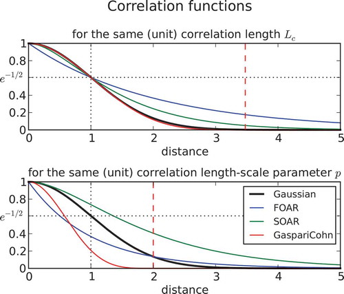
Several correlation model types have been used in data assimilation, such as the first-order autoregressive model (FOAR), the second-order autoregressive model (SOAR), the Gaussian model (G) and the compact support of order 5 of Gaspari and Cohn (1999) (GC) (see Appendix A for a description). These models are displayed in Figure 2. Each function actually depends on a length-scale parameter p of its own. The lower panel of Figure 2 shows the different correlation functions when the length-scale parameter is equal to unity for each function. We note that the decorrelation as a function of distance is very different from one model to another. In order to compare different correlation models and define a common measure of correlation length, an objective measure is needed. Pannekoucke et al. (2008) have reviewed different ways to define correlation length, and recommend using the one proposed by Daley (1991). The Daley’s correlation length is based on the curvature of the correlation function at the origin, that is, . For a Gaussian correlation model, , the correlation length defined by Daley (1991) actually matches the length-scale parameter . For distances equal to the correlation length, that is, , the Gaussian correlation function has a value equal to . This is the value we use to define the correlation length for the other correlation models. In this way, we can define for each correlation model a conversion factor between the correlation length and its model length-scale parameter. The conversion factors are as follow: for Gaussian correlation (by definition), for a FOAR, for a SOAR, and for a compact support Gaspari and Cohn correlation function. These conversion factors were obtained numerically by finding the zero of a nonlinear function. The upper panel of Figure 2 illustrates the different correlation models for the same unit correlation length. Note also that the shape of the Gaspari and Cohn function is very close to a Gaussian function, but goes to exactly zero at a distance . Overall, we emphasize that we should not confuse the correlation length-scale parameter of a model with its correlation length.

Figure 2. Correlation functions as a function of the (dimensionless) distance for common correlations models. The lower panel displays the distance dependence when the length-scale parameter of the individual models is set to unity. The upper panel shows the correlation functions when the length-scale parameter has been scaled to provide the same (unit) correlation length based on the Gaussian correlation model. Note that the solid black line (Gaussian) is identical in both panels. The vertical dashed line represents the distance at which the compact support correlation of Gaspari and Cohn is equal to zero.

The innovations, i.e. observation-minus-model residuals (denoted by d), are the information from which we can estimate error covariance model parameters. In the introduction we explained in simple terms how the observation-minus-model residuals actually contain information about the observation and background error variances as well as the model error correlation. In what follows we describe in mathematical terms the covariance model of the innovations and how to estimate their parameters, in particular the correlation length using three different methods.

First, we assume that innovations statistics vary with location and hour of the day, but are otherwise stationary for the same hour over the past several days (say, a month). The innovation variance at station i is modeled as

(1)

where and are the true error variances for observations and background (or model) at the station i, while , are the modeled (or estimated) observation and background error variances. The innovation covariance between a pair of stations is modeled as

(2)

where is a correlation length-scale parameter, and is the modeled background error correlation, assumed to be homogeneous and isotropic and thus depending only on the distance . The true background error correlation, on the other hand, could be nonhomogeneous. In eq 1 and eq 2 we assume that the observation errors are both spatially uncorrelated and independent of the background errors. We also assume that the statistics are stationary although they could have a diurnal variability. However, note that we are not assuming spatially uniform error variances; in fact, we allow them to be different at each observation sites and to vary with the hour of the day.

The Hollingsworth–Lönnberg method

The Hollingsworth–Lönnberg method (HL) is a well-established method developed for optimum interpolation (Rutherford, 1972; Hollingsworth and Lönnberg, 1986). The method estimates the background error variance and the correlation length (or the length-scale parameter p) by using a nonlinear square fit of a prescribed model error correlation model that depends only on distance against the sample covariance of innovations between a pair of stations i and j. In general, the fit consists of minimizing a cost function of the form

(3)

where s is a variance parameter and p is a correlation length-scale parameter, and a covariance normalization. There are in fact several algorithms possible, depending on the covariance normalization used and related interpretation of s (see Appendix B for details). For example, if then the estimate of the variance parameter represents the global mean background error variance, .

We can also devise a local fit and local estimation from eq 3 if the summation is done over all for a given , instead of summing over all pairs of stations . This then provides a local estimate of the variance parameter and of the correlation length-scale parameter at each observation site. We refer to this method as the local HL method. In its implementation, it is beneficial to use the following normalization , in which case the estimated variance parameter represents the estimated background error variance normalized by the innovation variance at the station, that is, . 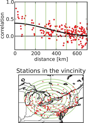Figure 3 shows an example of such a local fit using a Gaspari and Cohn correlation function for the Toronto North station. The lower panel displays the neighboring stations by circles of 100 km, and the upper panel shows the normalized sample innovation covariance and resulting fit in solid black. The intercept at the origin represents . Note also that the autocorrelation of the station Toronto North with itself is not displayed but should be exactly 1 at 0 distance.

Figure 3. Example of a local Hollingsworth–Lönnberg fit of a Gaspari and Cohn correlation function for O₃ around the station Toronto North (corner of Yonge and Finch avenues) for July 2014, 16 UTC. The lower panel shows the surrounding stations where innovations are collected, with concentric circles of 100 km apart (in light green). The upper panel shows the normalized autocovariance function as function of radial distance. The fitted correlation function is displayed with a solid black line.

When such a local estimation procedure is done at each stations, the background error variances of all the stations can be used to fit a unique and globally fitted correlation length-scale parameter—a procedure we call the global HL method. Details are given in Appendix B (eq B.3).

The maximum likelihood method

Aside from Baye’s estimation and least squares, the maximum likelihood estimation is one of the most important estimation methods. The maximum likelihood (ML) method is based on the principle that an estimate of a parameter θ (e.g., a parameter of a covariance model) can be made by finding the most plausible value, in terms of probability, of this parameter, given a set of observational data. The maximum likelihood method has many important properties that makes it quite powerful, one of which is that for a large number of observational data, the maximum likelihood estimate (and under fairly general assumptions), is asymptotically normally distributed. Thus, using a normal distribution for the parameter, one can get an analytical form for the log of the likelihood function. For a short introduction to the method, see for example Priestly (1981, §5.2) or Lupton (1993).

In our application, the observational data are the innovations , and the parameter we are trying to estimate is the correlation length-scale parameter p. We maximize the likelihood function or in practice minimize the log-likelihood function, which has the form

(4)

as shown in Dee and DaSilva (1999, section 4(a)).

The diagnostic method

When then

(5)

is known as the diagnostic condition (Talagrand, 1998; Ménard et al., 2000; Ménard and Chang, 2000). Note that the dimension of matrices are . The diagnostic condition has been used to estimate error variance and correlation length when one or the other is known. In our case, we use error variances estimated by the HL method, for determining the correlation length from the diagnostic equation, eq (5).

Results

Let us apply these methods first with a one-dimensional (1D) example where we know the true correlation length, and then to the Airnow observation network for O₃, PM_2.5, and NO₂ . In each of these experiments we estimate the model (or background) error variance and observation error variance at each observation station. This is done by using the local HL method. With these variance estimates we then estimate the correlation length using different methods, usually with a spatially homogeneous model, thus providing a single global value for the correlation length. However, the local HL method also provides locally fitted correlation lengths. We examine how the estimates of locally fitted correlation lengths and their statistics (mean, median, and harmonic mean) are relevant to the globally fitted correlation length estimates.

1D example

Consider a 1D domain of length , which mimics the east–west coverage of the AirNow observation network. Let us assume that there is an observation site at each grid point 100 km apart, so there are in total 45 observation sites. The Airnow observation network is very inhomogeneous, and we have not attempted to define what would be a median or average distance between observations. Nevertheless, considering that the objective analysis uses about 1,300 O₃ observations over an area of ~4,500 x 2,500 km² (east coast to west coast and from Houston to Winnipeg), then if these observations were to be distributed uniformly, this would give a linear observation density of 93 km for O₃. Although not essential, we furthermore assume that the domain is periodic in order to avoid dealing with the boundaries.

We seek to model the background error covariance with a spatially varying error variance and a homogeneous isotropic GC correlation model. The true background error correlation is also modeled with a GC function, but we allow having either a homogeneous or a nonhomogeneous formulation. For the homogeneous model, we consider length-scales of and 200 km. To construct a nonhomogeneous correlation model, we use a deformation of the coordinate system. This idea was discussed by Gaspari and Cohn (1999) and has been used by many to generate nonhomogeneous correlation models (e.g., Daley and Barker, 2001; Štajner et al., 2001; Segers et al., 2005; Pannekoucke et al., 2014). Here we use the displaced coordinate , given by

(6)

which results in a one-to-one mapping as long as . The way to build a nonhomogeneous correlation model in x space is to set the correlation model to be homogeneous and isotropic in the displaced coordinate system and then obtain the correlation model in x space by the change of coordinate in eq 6. A local correlation length can also be calculated from the transformation in eq 6 and is given as (see Appendix B for a derivation)

(7)

In our experimental setup, the value of α needs to be smaller than 7.16 in order to have a one-to-one mapping . We actually choose as it gives a range of length-scales with a ratio of largest/smallest length-scale of that we consider being in the ballpark of the experimental results we obtained with the AirNow observing network (results to be shown in the next subsection). Figure 4 shows an example of nonhomogeneous correlation with a GC model with length-scale of 500 km ( = 0.11). The length-scale used for this illustration is rather large and has been chosen for display purposes only.

Figure 4. One-dimensional nonhomogeneous model. Left, coordinate transformation . Right, resulting nonhomogeneous correlation (with , p = 0.11, L_c = 500 km in the displaced coordinate equation, eq 7). Contour isolines (0.2, 0.4, 0.6, 0.8, 1.0).

In the first series of simulations, we assume that the true error correlation is homogeneous and isotropic, while the background error variance is not uniform. Specifically, we set the standard deviation , where has an amplitude of 0.1. Figure 5 shows the result of a local HL fit using eq B.2 with uniform normalization (see Appendix B). The true error statistics are depicted with squares, and the estimated values with circles. The true background error variance has a wavenumber 5, which corresponds to length-scale variability of 450 km (4,500 km/2 × wavenumber), and the true background error correlation length is uniform with a value of 100 km. We note that despite the nonuniformity of the variance field, both the background error variance and background error correlation length converge to the truth. Next, we consider random spatial variations of the background error variance on the grid, and thus with no coherent spatial distribution of background error from one observation site to the next. Figure 6 shows the results of the local HL estimation with a standard deviation of set to . Results show fairly accurate estimation of the correlation length with an error of the order of 2% only, which we compute by taking the standard deviation of the correlation error estimate and divide by the mean true correlation length. However, the estimated background error variance does not match the true (random) background error. The estimation error standard deviation is about 15%. We also note that the estimated error variance is smoother than the true background error variance.

Figure 5. HL local estimates for and . The true background error has an homogneous isotropic correlation and spatially varying variance (wavenumber 5). Squares are the true values, and filled circles are the HL estimates.

Figure 6. HL local estimates for and . The true background error has a homogeneous isotropic correlation with a spatially uncorrelated (random) background error variance. Squares are the true values, and filled circles are the HL estimates.

The estimated error variances were used to prescribe the error variances in a maximum likelihood (ML) estimation of the correlation length by minimizing the log-likelihood function of eq 4. The ML estimates are also very close to the truth: = 100 km for the experiment in Figure 5, and = 99 km for the experiment in Figure 6.

In a second series of experiments depicted in Figures 7 and 8, the previous experiments are repeated but with the difference that the nonhomogeneous error correlation model is used to represent the truth. In the case of a periodic perturbation of the background error variance, in Figure 7, the estimation error is less than 2% for the background error variance and 4% for the local correlation length. Next, we consider spatially random perturbations of the background error variance, in Figure 8. The mean relative estimation error of the error variance is of the order of 2% but its standard deviation is about 12%. Again, we note that the estimated error variance is spatially smoother than the true error variance. The mean relative error of the local correlation length is less than 1% and its relative standard deviation error is about 5%.

Figure 7. Same as Figure 5 but for a nonhomogeneous error correlation for the truth.

Figure 8. Same as Figure 6 but for a nonhomogeneous error correlation for the truth.

We then use the estimated error variances in a ML estimation to estimate a global correlation length. The correlation model used being homogeneous and isotropic and thus described by a single correlation length number. In effect, this situation is prevalent in reality where we try to fit a homogeneous isotropic correlation model with the truth. For the periodic error variances case, the maximum likelihood correlation length is = 104 km, while the random error variance case gives = 103 km. These estimates are close to the correlation length . If we try to characterize the HL local correlation length by a single number, for example, the mean value, we get a value of 120 km in both experiments, which is much larger than . Figure 9 depicts these results. It is also interesting to derive a correlation length based on the eq 7. If we take the harmonic mean of and consider the fact that we get , which is the correlation length in the displaced coordinate system. In our 1D simulation experiment this correlation length is nearly identical to (result not displayed in Figure 9). The estimated correlation length using the estimated error variance was also computed, and is represented with the solid black line. Note that at 91 km. Note also that the function is also equal to 1 at = 0, and thus is not monotonic and reaches a minimum between = 0 and . Actually, this non-monotonic behavior is seen in all experiments, as in the case where the variance is uniform and the true correlation is homogeneous and isotropic (result not shown). Moreover, as we change the number of observations, the location of the minimum of also changes, whereas the maximum likelihood estimate is roughly independent of the number of observations. The minimum of thus appears to be a numerical artifact that has no physical meaning. It is also always smaller than the true correlation length. Overall, the minimum of cannot be used as an estimator of the correlation length.

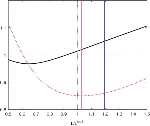
Figure 9. Different correlation length estimates. Spatially random error variance with nonhomogeneous error correlation as in Figure 8. Dotted-pink line represents the log-likelihood function, and in solid pink the minimum of the log-likelihood function. The mean HL local correlation length is in blue. The for different modeled correlation lengths (in abcissa) is represented with a solid black line. The ordinate are values of .

Finally, we remark that the local HL estimation of error variance and correlation length is deficient in certain cases where we observe that the minimum of the cost function is degenerate: having a flat curvature in one direction, like an elongated valley. We have identified two cases when this happens. One is when the error variance is near zero; the estimation of the correlation length fails to converge and basically remains at its initial guess value. A second case arises when the length-scale is small, and in particular when there are six observation stations (or data points) or less within the spatial range of nonzero values of the GC model. This seems to be related to the fact that six data points are needed to fit a polynomial of order 5 of the GC function. Although further investigation would be needed to provide further understanding of this issue, in practice we identify a degenerate estimate when we observe that HL correlation-length estimates depend on the initial guess value of the minimization algorithm. The estimated error variance is also erroneous in that case.

Estimation of correlation length in the context of the OA of Airnow observations

Dealing with real data requires careful statistical treatment due to missing data and outliers. The presence of outlier data can have a large impact on the estimation of variances and is detrimental in least-squares fit (e.g., Tarantola, 1987, example problem 1.9). Thus, we first discuss these issues and then the implementation of the HL method in order to get estimates of the background error variance. Once we have error variance estimates, we can then investigate the different methods for estimating the correlation length.

In our experiments, innovations are collected at each hour for each observation site for a period of 60 days. The error variance and correlation length estimate should be, in principle, derived with respect to this 60-day sampling period, but due to missing data and quality control (to be detailed shortly), time series of innovations at a site for a given hour result in having less than 60 data points, and the statistics need to carefully account for this fact.

First, a gross check on the observed values is introduced: Observations with unrealistically large or negative values are removed. A gross check on the innovation is also introduced: Any innovation that exceeds a certain cutoff value is discarded from the time series. The cutoff values are set to 50 ppbv for O₃, 30 ppbv for NO₂ and SO₂, and 100 for PM_2.5 and PM₁₀. As we calculate variances and covariances of innovations, the mean value needs to be removed from the time series of innovations. The length of the time series is calculated after all the gross checks are applied, and varies from station to station and from hour to hour. The removal of the mean is further complicated when we calculate the covariance between two time series from two stations. For example, missing data at one site may occur on a set of days that are different from the days of missing data at another site. To calculate a covariance between a pair of time series, we require that pairs of data to be formed each day in order to compute the statistics. This pairing on a daily basis has an impact on the number of data in the paired time series and on the computation of the mean at each paired stations. The mean calculated at paired stations may differ from the mean used at a single station to calculate the error variance, for example. As a result, the length of time series varies from station to station, hour to hour, and is different for different pairs of time series. For all the statistics, we set to a minimum of 30 the number of data points needed to infer the statistics. If there are less than 30 instances at a given hour at a given location or for given pair of stations, then the time series in question is not used at all. When this filtering and data manipulation are completed, the data can then be used for statistical estimation.

We first apply a local HL estimation method at each station and at each hour using a GC correlation model. We thus obtain the observation and background error variances, , as well as the local correlation length at each station and for each hour. We then compute the distribution of at a given hour. From these distributions we compute the median, the first and third quartile (), and the mean. We use the difference between the third and first quartile as a robust measure of spread. Then we remove outliers in the correlation length estimates obtained from the HL method. Any correlation length estimate that is smaller than or larger than is considered an outlier and the data related to this station at this hour are not further used in computing the statistics, since too long or too short correlation lengths, resulting from HL faulty fits, may also give erroneous error variances. 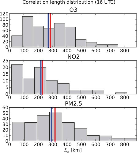Figure 10 shows the resulting (filtered) distribution of at 16 UTC. The blue line represents the median value and the red one the mean value. This filtered data set is used in all following global correlation length estimation experiments.

Figure 10. Distribution of the local Hollingsworth–Lönnberg correlation length estimates for O₃, NO₂, and PM_2.5 using the filtered data at 16 UTC. The blue lines represent the median and the red line the mean value.

Having the observation and background error variance estimates, we can now form the background error correlation and estimate a global correlation length that fits all the data. Note that a single correlation length is needed for the analysis, while the local HL has given us a whole range of values. We could use, of course, the median or the mean value of the distribution, but there are also other approaches to consider: a global Hollingsworth–Lönnberg (HL) method, the maximum likelihood (ML) method, and a method based on diagnostic.

In the global HL, the fit to a correlation model is done with respect to all pairs of stations as a function of distance, and there is thus no reference to a station in particular. If the error variance field could be considered spatially homogeneous, this procedure would also give a globally valid observation and background error variance as in eq 3, but we do not make this assumption here as there is significant spatial variability in the background error variance field. The issue of spatial variability of the error variances in a global HL procedure can be alleviated if the sampled innovation covariance is normalized with background error standard deviation as in eq B.3 (see Appendix B). The intercept at the origin of the fitted correlation function is then, by construction, equal to 1. This approach was used to construct our global HL estimate of the correlation length. Another global approach consists of applying the maximum likelihood of a homogeneous and isotropic covariance model given the covariance of innovations. As with other methods considered here, the local HL estimates of observation and background error variances are used in the correlation estimation. The ML method is then applied to estimate a single parameter: the global correlation length, which we denote by . Finally, we obtain a global estimate of the correlation length is based on the criterion (Ménard and Chang, 2000).

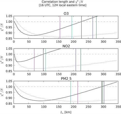
Figure 11 shows the results of estimating the global correlation length for O₃, PM_2.5, and NO₂ from the three global estimation methods just described, using data from the period June 14 to August 12, 2014. The values of are plotted in solid black, the log-likelihood function is plotted in dotted pink, and the minimum of the log-likelihood (i.e., maximum likelihood) is plotted as a vertical pink line. Note that the values of the log-likelihood are not plotted on these graphics, as the actual values are in fact irrelevant, but only the shape of the log-likelihood function is displayed, indicating the location of the minimum. The result of global HL fit is depicted in green. The median of the local HL distribution is displayed in blue. We have also displayed a global correlation length-scale that is derived from a mean of inverse correlation lengths (or harmonic mean) depicted in cyan, that is, . The results are also summarized in Table 2. We note that global HL and median local HL correlation length are significantly larger than the maximum likelihood estimates, as in the 1D simulated case. The correlation length estimation based on the criterion also lies somewhere in between. As discussed in the 1D simulation, the fact that the global correlation length estimates from HL, ML, and differ is an indication that the true correlation is nonhomogeneous. We have also noted in the 1D simulation that the ML estimate is closer to the correlation length in the un-deformed coordinate system, and thus has a physical meaning. We could perhaps infer that in this real data case, the ML estimation has also a physical meaning. We show in the next paragraph that the ML estimates actually exhibit a diurnal variation, which one could argue to be physical. Finally, the HL harmonic mean correlation length-scale is larger than the ML estimate for O₂ and NO₂ and closer to the estimate, but not for PM_2.5.

Table 2. Correlation length estimates (km) from different methods, July 2014, 16 UTC.

Species	Maximum likelihood	HL harmonic mean		HL global	Median HL
O3	155	195	227	277	265
PM2.5	215	191	295	297	303
NO2	69	107	99	225	208

Figure 11. Comparison of different correlation length estimates for O₃, NO₂, and PM_2.5 at 16 UTC for the summer 2014. in solid black, the log-likelihood function (rescaled) in dotted pink, the maximum likelihood estimate in solid pink, the global HL estimate in green, the median HL in blue, and the harmonic mean HL is in cyan.

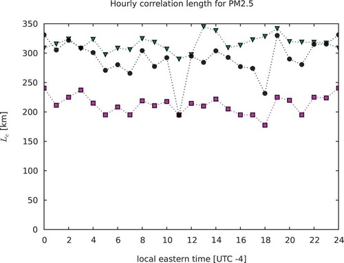
These estimation methods were also conducted for a whole diurnal cycle. The results are illustrated in Figures 12, 13, and 14, where the pink squares are the ML estimates, the black circles the method estimates, and the green triangles the global HL estimates. We note that the correlation length for PM_2.5 has no diurnal signal, while O₃ has a weak one and NO₂ has a strong one. The global HL estimates for NO₂ show a weaker diurnal signal. It thus seems that the global HL correlation length is less physical and maybe overestimated. The correlation length based on does, however, show a diurnal variability that is quite similar to the ML estimate especially for the NO₂. However, it has a tendency to be larger, and actually comparable to the global HL estimates in the case of PM_2.5. Finally, we should remark that these estimates were obtained in UTC time, not in local time. There is 3½ hours of time zone difference in the GEM-MACH domain. Thus, the diurnal signature is then convoluted by the local time at a given UTC time. The net effect also depends on the spatial inhomogeneity distribution of the observation network, which is quite significant for NO₂.

Figure 12. Time evolution of the correlation length for O₃. Maximum likelihood estimates in pink, estimates in black, and global HL in green.

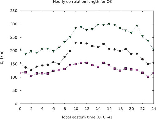
Figure 13. Time evolution of the correlation length for NO₂. Maximum likelihood estimates in pink, estimates in black, and global HL in green.

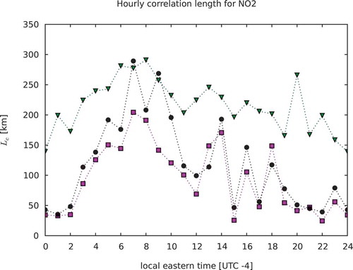
Figure 14. Time evolution of the correlation length for PM_2.5. Maximum likelihood estimates in pink, estimates in black, and global HL in green.

Summary and conclusions

We present some preliminary work for our next phase of development of the objective analysis of surface pollutants. We focus on a study of the methods to estimate the error variances at each observation sites and estimate a globally valid error correlation length. We first argue in favor of using compact support correlation functions on the basis that, first, it considerably speeds up the computation of the analysis; second, because the monthly sample of innovation spatial auto-covariance is noisy at large distances and it is unclear how useful this data can be used to estimate the tails of the correlation functions; and finally, in view of our planned development based on ensemble assimilation where spatial localization is an essential part, the information about correlations past a certain distance is never used in the analysis solver anyway. We thus conclude that there is apparently no real need to have correlation functions defined over an infinite range, and we thus propose to use compact support correlation functions for both estimation and modeling.

We then consider three estimation methods: the Hollingsworth–Lönnberg (HL) method, the maximum likelihood (ML) method, and the method based on the diagnostic. Other methods such as the NMC method (Parrish and Derber, 1992) or the ensemble of assimilation method (Fisher, 2003; for a review see also Bannister, 2008) cannot be applied here, since our analyses are off-line; they are not part, yet, of an assimilation cycle.

Then we use a local Hollingsworth–Lönnberg fit to estimate error variances and error correlation at each station, and test the validity of this approach using a simplified 1D observation network where the true statistics are known. The use of 1D observing networks has been a testbed to validate error statistics estimation methodologies by several authors (e.g., Desroziers et al., 2005; Ménard, 2016; Waller et al., 2015), but here we allow error variances being different at each observation site. We examined cases where the error variances vary spatially in a regular fashion or, in the other extreme, as a spatially uncorrelated random field. The true error correlation can also be either homogeneous or nonhomogeneous using a deformation of the coordinate system. Before estimating the correlation length, we first use a local HL method to estimate the background error variances at each observation station. We note that the spatial variability of the background error variance is estimated quite accurately at each observation site as long as the spatial length-scale variability of the error variance is not smaller than the correlation length. In the opposite case, where it is smaller than the correlation length, the estimated error variances at each site have some error but they nevertheless provide an estimated variance field that is somewhat smoother than the true error variance. The local HL estimation method also gives a generally accurate estimates of the correlation length for both homogeneous and nonhomogeneous correlation models, as long as the spatial variability of the nonhomogeneous correlation remains larger than the correlation length. This is the case in these experiments and explains why the correlation length estimates are accurate.

Using the estimated error variances at each of the 1D observation sites, we construct an error correlation and then fit data with a homogeneous error correlation model using different methods. We compare some statistics (mean and harmonic mean) of the estimates obtained using the local Hollingworth–Lönnberg method with the globally valid estimates obtained from the maximum likelihood method and the diagnostic. When the true error correlation is itself homogeneous and isotropic, all three correlation length estimates are identical to the true correlation length. The problems arise when the true error correlation is nonhomogeneous, and then different methods give different globally valid correlation lengths. The maximum likelihood estimate gives a correlation length that is close to the correlation length used in the original un-displaced coordinate system (which was used to generate the nonhomogeneous error correlation in the first place). The mean value of the local HL estimates yield correlation lengths that are the largest, and the correlation length based on satisfying the is different but a bit closer to the maximum likelihood estimate.

We then applied these methods to real data using the GEM-MACH model output and the AirNow observations of O₃, NO₂, and PM_2.5 for a summer case. As in the simulated case, the background error variances are obtained using a local HL estimation method; then a sample correlation is computed and we fit a homogeneous-isotropic correlation model to obtain a globally valid correlation length estimates. This is done using three methods: the global HL method, the maximum likelihood method, and the method. As in the simulated case, the global HL method gives the largest correlation length, with values comparable to the median of the local HL estimates. The maximum likelihood gives the smallest values, and the method gives values somewhere in between. To see if we can capture some physical significance of these estimates, we examine the diurnal variation of the different correlation length estimates for O₃, NO₂, and PM_2.5. We found that the maximum likelihood and the methods are able to capture the diurnal variability of the correlation length for O₃ and NO₂, which is particularly strong. For PM_2.5 we found no diurnal variability in all methods. The maximum likelihood estimate also gives the smallest value, while the global HL gives the largest values and the method somewhere in between.

In summary, we conclude from both simulations and using real data, that the maximum likelihood method gives the smallest and a physically reasonable estimate of correlation length and captures well the diurnal variability in real data and the underlying un-displaced correlation length in simulated data. The global HL or the median value of local HL gives the largest global correlation lengths, which seem unrealistically large.

We stress that the estimated covariance parameters were obtained with off-line analyses, and are thus related directly to the GEM-MACH model output, and not to the observation network. These global correlation lengths give, for example, an idea of an upper bound of the largest distance that observation sites can be separated to form a meaningful analysis. When the distance between observations exceeds this value, there are regions where observations play no role in the analysis. Our results thus indicate that the distance between O₃ observations should not exceed both 100–150 km. Likewise, PM_2.5 sites should not be separated by much more than 200 km, while the exceeding distances for NO₂ sites have a strong diurnal variation from 50 to 150 km. It is important to emphasize that these length-scales are only upper bounds and cannot define an optimum density of an observation network, since spatial details and temporal events that are not statistical in nature may not be captured with these statistical estimation procedures. The error variance estimated by the local HL can also give an idea of the statistical random uncertainty of the GEM-MACH model, where the observation noise has been effectively removed out the observed-minus-forecast differences.

For data assimilation, this study indicates that the error variances can be reasonably estimated at the observation sites and that one of the greatest limitations comes from using homogeneous error correlations. Consequently, a significant improvement of the analysis should come from using nonhomogeneous modeling of the background error correlation.

Now let’s consider the limitations of this study. First, the error variances we have estimated are not definitive, as they are dependent on the type of correlation model we used, namely the compactly supported GC model. This choice of model has been made because it is widely used in data assimilation. However, the underlying stochastic process of a GC model is in fact spatially smooth and may not be appropriate to represent the spatial variability of O₃, NO₂, and PM_2.5 in the boundary layer. In the future we shall investigate other compact support correlation functions, in particular, exponential-like correlation functions that are not differentiable at the origin. Such verification requires the production of an analysis, and there are yet other components of an analysis that needs to be completed and validated before this could be done.

Acknowledgment

The authors thank Jean de Grandpré and Heather Morrison for the review of the paper, and as well as two anonymous reviewers for their comments, which greatly helped made this paper accessible to a wider audience.

Additional information

Notes on contributors

Richard Ménard

Richard Ménard is a research scientist and Martin Deshaies-Jacques is a specialist in physical sciences, both at the Modeling and Integration section of the Air Quality Research Division in Dorval, Québec, Canada.

Martin Deshaies-Jacques

Richard Ménard is a research scientist and Martin Deshaies-Jacques is a specialist in physical sciences, both at the Modeling and Integration section of the Air Quality Research Division in Dorval, Québec, Canada.

Nicolas Gasset

Nicolas Gasset is a postdoctoral fellow at the Environmental Numerical Weather Prediction Research section of the Meteorological Research Division in Dorval, Québec, Canada.

Appendix A—Correlation functions

Gaspari and Cohn (1999) provide the theory and practical examples on how to construct compactly supported correlation functions by self-convolution of space-limited functions. They also give a practical way to construct correlation functions on the surface of a sphere by using a valid correlation function in R³ but using it only on a spherical manifold subdomain of R³. Homogenous isotropic correlation functions on the surface of a sphere are then radially symmetric functions, that is, depend only on where x and y are position vectors in R³, but confined to the surface of a sphere. The distance is then the chordal distance between two points on a sphere, not to be confused with the great circle distance.

The Gaussian correlation function is given as

The first-order autoregressive model is given as

The second-order autoregressive model is given as

and the fifth-order compact support correlation function of Gaspari and Cohn is given as

Appendix B—The Hollingsworth–Lönnberg method

The classical HL method consists of estimating and p by a nonlinear least-square fit (e.g., Levenberg–Marquardt algorithm) with a cost function of the form

(B.1)

where s is the intercept of the fitted correlation function at zero distance, and is the covariance of innovation between a pair of stations i and j. The least-square estimate then related to the background error variance . In its more general form (B.1), we introduce a covariance normalization that actually defines precisely what is. Generally the sum is done over all pairs of stations and the background error variance is a global estimate, but local estimates can also be obtained, say at a station i, by summing all j’s () for a given i. The least-square estimate is then related to the background error variance at the observation station, and the estimated correlation length-scale parameter is associated with a local estimate of the parameter.

Since in air quality applications the innovation variance may vary considerably from one observation site to the next, in the local version of (B.1) could also use a scaled cost function of the form

(B.2)

The estimated parameter then represents . The normalization by the innovation variance is introduced to reduce the spatial variability of the statistics. This is, of course, only an approximation and is best suited if the ratio is independent of location. The main issue with local HL estimation is that it does not provide a unique correlation length required by optimum interpolation to specify the correlation length of a homogeneous isotropic error correlation model.

A true fit to nonuniform error statistics would require a global fit to determine all background error variances at all observation site simultaneously along with a single p value. This would require searching for the minimum of a cost function of the form , which can be a daunting task, if at all a well-posed problem. In practice we use an alternative and approximate approach. First we use eq B.2 to estimate the error background error variances at the observation stations, then use the following global HL fit with the cost function

(B.3)

to obtain a unique length-scale parameter estimate p. Here, by construction, the intercept at the origin is equal to 1.

Appendix C—Correlation length in the displaced coordinate system

Let us first derive an expression to relate the second derivative with respect to the radial distance with derivatives of the correlation function with respect to x and y. Consider a coordinate change from to a rotated coordinate system and and consider the correlation function expressed in this new rotated coordinate system,

(C.1)

where x and y are obtained by the inverse transformation . The first and second derivatives of C with respect to r are given by

(C.2)

(C.3)

Now consider a spatial displacement transformation of the form

(C.4)

so that

(C.5)

then we get for the first derivative

(C.6)

and for the second derivative,

(C.7)

(C.8)

(C.9)

Now we can compute the second derivative of with respect to r using eq C.3 and eqs C.7–C.9. At or we have

(C.10)

so that the second derivative at becomes

(C.11)

As we define the correlation length with the curvature, and we set it to in the displaced transformed coordinate system, that is,

(C.12)

the local correlation length in the original coordinate system is then given as

(C.13)

References

- Bannister, R.N. 2008. A review of forecast error covariance statistics in atmospheric variational data assimilation. I: Characteristics and measurements of forecast error covariances. Q. J. R. Meteorol. Soc., 134:1951–70. doi:10.1002/qj.339
- Bocquet, M., H. Elbern, H. Eskes, M. Hirtl. R. Žabkar, G.R. Carmichael, J. Flemming, A. Inness, M. Pagowski, J.L. Pérez Camaño, P.E. Saide, R. San Jose, M. Sofiev, J. Vira, A. Baklanov, C. Carnevale, G. Grell, and C. Seigneur. 2015. Data assimilation in atmospheric chemistry models: Current status and future prospects for coupled chemistry meteorology models. Atmos. Chem. Phys. 15:5325–58. www.atmos-chem-phys.net/15/5325/2015. doi:10.5194/acp-15-5325-2015
- Bouttier, F. 1994. Sur la prévision de la qualité des prévisions météorologiques. Ph.D. dissertation, Université Paul Sabatier, 240 pp. [Available from Université Paul Sabatier, Toulouse, France.]
- Buehner, M., R. McTaggart-Cowan, A. Beaulne, C. Charette, L. Garand, S. Heilliette. E. Lapalme, S. Laroche, S.R. Macpherson, J. Morneau, and A. Zadra. 2015. Implementation of a deterministic weather forecasting system based on ensemble-variational data assimilation at Environment Canada. Part I: The global system. Monthly Weather Rev. 143:2532–59. doi:10.1175/MWR-D-14-00354.1
- Caron, J.-F., T. Milewski, M. Buehner, R. L. Fillion, M. Reszka, S.R. Macpherson, and J. St-James. 2015. Implementation of a deterministic weather forecasting system based on ensemble-variational data assimilation at Environment Canada. Part II: The regional system. Monthly Weather Rev. 143:2560–80. doi:10.1175/MWR-D-14-00353.1
- Chai, T., G.R. Carmichael, Y. Tang, A. Sandu, M. Hardesty, P. Pilewskie, S. Whitlow, E.V. Browel, M.A. Avery, P. Nédélec, J.T. Merrill, A.M. Thompson, and E. Williams. 2007. Four-dimensional data assimilation experiments with International Consortium for Atmospheric Research on Transport and Transformation ozone measurements. J. Geophys. Res. 112:D12S15. doi:10.1029/2006JD007763,2007
- Crouze, D.L., P.A. Peters, P. Hystad, J.R. Brook, A. van Donkelaar, R.V. Martin, P.J. Villeneuve, M. Jerrett, M.S. Goldberg, C.A. Pope III, M. Brauer, R.D. Brook, A. Robichaud, R. Ménard, R.T. Burnett. 2014. Ambient PM2.5, O3, and NO2 exposures and association with mortality over 16 years of follow-up in the Canadian Census Health and Environment Cohort (CanCHEC). Environ. Health Perspect. 123:1180–86. doi:10.1289/ehp.1409276( accessedNovember2, 2015)
- Daley, R. 1991: Atmospheric Data Analysis. New York, NY: Cambridge University Press.
- Daley, R., and R. Ménard. 1993. Spectral characteristics of Kalman filter systems for atmospheric data assimilation. Monthly Weather Rev. 121:1554–65. doi:10.1175/1520-0493(1993)121%3C1554:SCOKFS%3E2.0.CO;2
- Daley, R, and E. Barker. 2001. NAVDAS: formulation and diagnostics. Monthly Weather Rev. 129:869–83. doi:10.1175/1520-0493(2001)129<0869:NFAD>2.0.CO;2
- Dee, D.P., and A.M. da Silva, 1999a. Maximum likelihood estimation of forecast and observation error covariance parameters. Part I. Methodology. Monthly Weather Rev. 127:1822–34. doi:10.1175/1520-0493(1999)127%3C1822:MLEOFA%3E2.0.CO;2
- Dee, D.P., and A.M. da Silva, 1999b. Maximum likelihood estimation of forecast and observation error covariance parameters. Part II. Applications. Monthly Weather Rev. 127:1835–49. doi:10.1175/1520-0493(1999)127%3C1835:MLEOFA%3E2.0.CO;2
- Desroziers, G., L. Berre, B. Chapnik, and P. Poli. 2005. Diagnostic of observation, background and analysis-error statistics in observation space. Q. J. R. Meteorol. Soc. 131:3385–96. doi:10.1256/qj.05.108.doi:10.1256/qj.05.108
- Elbern, H., and H. Schmidt. 2001. Ozone episode analysis for four-dimensional variational chemistry data assimilation. J. Geophys. Res. 106(D4):3569–90. doi:10.1029/2000JD900448
- Elbern, H., A. Strunk, H. Schmidt, and O. Talagrand. 2007. Emission rate and chemical state estimation by 4-dimensional variational inversion. Atmos. Chem. Phys. 7:3749–69. www.atmos-chem-phys.net/7/3749/2007. doi:10.5194/acp-7-3749-2007
- Frydendall, J., J. Brandt, and J.H. Christensen. 2009. Implementation and testing of a simple data assimilation algorithm in the regional air pollution forecast model, DEOM. Atmos. Chem. Phys. 9:5475–88. www.atmos-chem-phys.net/9/5475/2009. doi:10.5194/acp-9-5475-2009
- Fisher, M. 2003. Background error covariance modeling. Proceedings of the ECMWF Seminar on recent developments in data assimilation for atmosphere and ocean, September 8–12, 2003. Reading, UK: ECMWF.
- Gaspari, G., and S.E. Cohn, 1999. Construction of correlation functions in two and three dimensions. Q. J. R. Meteorol. Soc. 125:723–57. doi:10.1002/(ISSN)1477-870X
- Gneiting, T. 2002. Compactly supported correlation functions. J. Multivariate Anal. 83:493–508. doi:10.1006/jmva.2001.2056
- Hoelzemann, H. Elbern, and A. Ebel. 2001. PSAS and 4D-var data assimilation for chemical state analysis by urban and rural observation sites. Phys. Chem. Earth (B) 26:807–812. doi:10.1016/S1464-1909(01)00089-2
- Hollingsworth, A., and P. Lönnberg. 1986. The statistical structure of short-range forecast errors as determined from radiosonde data. Part I: The wind field. Tellus A 38:111–36. doi:10.1111/j.1600-0870.1986.tb00460.x
- Houtekamer, P.L, and H.L. Mitchell. 2005. Ensemble Kalman filtering. Q. J. R. Meteorol. Soc. 131:3269–89. doi:10.1256/qj.05.135
- Lee, P., and Y. Liu. 2014. Preliminary evaluation of a regional atmospheric chemical data assimilation systems for environmental surveillance. Int. J. Environ. Res. Public Health 11:12795–816. doi:10.3390/ijerph111212795
- Lupton, R. 1993: Statistics in Theory and Practice. Princeton, NJ: Princeton University Press.
- Ménard, R. 2016. Error covariance estimation methods based on analysis residuals: Theoretical foundation and convergence properties derived from simplified observation networks. Q. J. R. Meteorol. Soc. 142:257–273. doi:10.1002/qj.2650.
- Ménard, R., and L.P. Chang. 2000. Assimilation of stratospheric chemical tracer observations using a Kalman filter. Part II: χ2-validated results and analysis of variance and correlation dynamics. Monthly Weather Rev. 128:2672–86. doi:10.1175/1520-0493(2000)128<2672:AOSCTO>2.0.CO;2
- Ménard, R., L.P. Chang and J.W. Larson. 2000. Application of a robust χ2 validation diagnostic in PSAS and Kalman filtering experiments. In Proceedings of the Third WMO International Symposium on Assimilation of Observations in Meteorology and Oceanography, WWRP Report Series No.2. WMO/TD – No 986. 404 pp. Quebec City, Canada, 7–11 June 1999. World Meteorological Organization.
- Ménard, R., and A. Robichaud. 2005. The chemistry-forecast system at the Meteorological Service of Canada. In ECMWF Seminar Proceedings on Global Earth-System Monitoring, September 5–9, 2005, Reading, UK, 297–308.
- Mitchell, H.L., and P.L. Houtekamer. 2000. An adaptative ensemble Kalman filter. Monthly Weather Rev. 128:416–33. doi:10.1175/1520-0493(2000)128<0416:AAEKF>2.0.CO;2
- Moran, M.D., S. Ménard, R. Pavlovic, D. Anselmo, S. Antonopoulus, A. Robichaud, S. Gravel, P.A. Makar, W. Gong, C. Stroud, J. Zhang, Q. Zheng, H. Landry, P.A. Beaulieu, S. Gilbert, J. Chen, and A. Kallaur. 2012. Recent advances in Canada’s national operational air quality forecasting system. 32nd NATO-SPS ITM, Utrecht, NL, May 7–11, 2012.
- Pagowski, M., G.A. Grell, S.A. McKeen, S.E. Peckham and D. Devenyi. 2010. Three-dimensional variational data assimilation of ozone and fine particulate matter observations: Some results using the Weather Research and Forecasting–Chemistry model and grid-point statistical interpolation. Q. J. R. Meteorol. Soc. 136:2013–24. doi:10.1002/qj.700
- Pannekoucke, O., L. Berre, and G. Desroziers. 2008. Background-error correlation length-scale estimates and their sampling statistics. Q. J. R. Meteorol. Soc. 134:497–508. doi:10.1002/qj.212
- Pannekoucke, O., E. Emili, and O. Thual. 2014. Modelling of local length-scale dynamics and isotropizing deformations. Q. J. R. Meteorol. Soc. 140:1387–98. doi:10.1002/qj.2204
- Parrish, D.F., and J.C. Derber. 1992. The National Meteorological Center’s spectral statistical interpolation analysis system. Monthly Weather Rev. 120:1747–63. doi:10.1175/1520-0493(1992)120<1747:TNMCSS>2.0.CO;2
- Priestley, M.B. 1981. Spectral Analysis and Time Series. Volume 1: Univariate Series. London, UK: Academic Press.
- Robichaud, A., and R. Ménard. 2014. Multi-year objective analysis of warm season ground-level ozone and PM2.5 over North America using real-time observations and Canadian operational air quality models. Atmos. Chem. Phys. 14:1769–800. doi:10.5194/acp-14-1769-2014
- Robichaud, A., R. Ménard, Y. Zaïtseva, and D. Anselmo. 2016. Multi-pollutant surface objective analyses and mapping of air quality health index over North America. Air Qual. Atmos. Health. in press. doi:10.1007s11869-015-0385-9.
- Rösevall, J.D., D.P. Murtagh, J. Urban, and A.K. Jones. 2007. A study of polar ozone depletion based on sequential assimilation of satellite data from the ENVISAT/MIPAS and Odin/SMR instruments. Atmos. Chem. Phys. 7:899–911. www.atmos-chem-phys.net/7/899/2007/( accessed February 16, 2007). doi:10.5194/acp-7-899-2007
- Rutherford, I. 1972. Data assimilation by statistical interpolation of forecast error fields. J. Atmos. Sci. 29:809–15. doi:10.1175/1520-0469(1972)029<0809:DABSIO>2.0.CO;2
- Sandu, A., and T. Chai, 2011: Chemical data assimilation—An overview. Atmosphere 2:426–63. doi:10.3390/atmos2030426
- Segers, A.J., H.J. Eskes, R.J. van der A, R.F. van Oss, and P.F.J. van Velthoven. 2005. Assimilation of GOME ozone profiles and a global chemistry-transport model using a Kalman filter with anisotropic covariance. Q. J. R. Meteorol. Soc. 131: 477–502. doi:10.1256/qj.04.92
- Silibello, C., A. Bolingnano, R. Sozzi, and C. Gariazzo. 2014. Application of a chemical transport model and optimized data assimilation methods to improve air quality assessment. Air Qual. Atmos. Health. 7: 283–296. doi:10.1007/s11869-014-0235-1.
- Singh, K, M. Jardak, A. Sandu, K. Bowman, M. Lee, and D. Jones. 2011. Construction of non-diagonal background error covariance matrices for global chemical data assimilation. Geosci. Model Dev. 4:299–316. doi:10.5194/gmd-4-299-2011
- Štajner, I., L.P. Riishøjgaard, and R.B. Rood. 2001. The GEOS ozone data assimilation system: Specification of error statistics. Q. J. R. Meteorol. Soc. 127:1069–94. doi:10.1002/(ISSN)1477-870X
- Stieb, D.M., R.T. Burnett, M. Smith-Dorion, O. Brion, H.H. Shin, and V. Economou. 2008. A new multipollutant, no-threshold air quality health index based on short-term associations observed in a daily time-series analyses. J. Air Waste Manage. Assoc. 58:435–50. doi:10.3155/1047-3289,58.3,3,435
- Talagrand, O. 1998. A posteriori evaluation and verification of analysis and assimilation algorithms. Proceedings of the Workshop on Diagnostics of Data Assimilation Systems, pp. 17–28, ECMWF, England, November 2–4, 1998.
- Tanborn, A., R. Ménard, and D. Ortland. 2002. Bias correction and random error characterization for the assimilation of high-resolution Doppler imager line of sight velocity measurements. J. Geophys. Res. 107(D12): 4147. doi: 10.1029/2001JD000397
- Tarantola, A. 1987. Inverse Problem Theory: Methods for Data Fitting and Model Parameter Estimation. Amsterdam, The Netherlands: Elsevier.
- Tilmes, S. 2001. Quantitative estimation of surface ozone observation and forecast errors. Phys. Chem. Earth (B) 26:759–62. doi:10.1016/S1464-1909(01)00082-X
- Tombette, M., V. Mallet, and B. Sportisse. 2009. PM10 data assimilation over Europe with optimal interpolation method. Atmos. Chem. Phys. 9:57–70. www.atmos-chem-phys.net/9/57/2009 ( accessed January 7, 2009).
- Waller, J.A., S.L. Dance, and N.K. Nichols. 2015. Theoretical insight in diagnosing observation error correlations using observed-minus-background and observed-minus analysis statistics. Q. J. R. Meteorol. Soc. doi:10.1002/qj.2661 ( accessed October 26, 2015).
- Wu, L. V. Mallet, M. Bocquet, and B. Sportisse. 2008. A comparison study of data assimilation algorithms for ozone forecasting. J. Geophys. Res. 113(D20310). doi:10.1029/2008JD009991.