South Philadelphia passive sampler and sensor study

ABSTRACT

From June 2013 to March 2015, in total 41 passive sampler deployments of 2 wk duration each were conducted at 17 sites in South Philadelphia, PA, with results for benzene discussed here. Complementary time-resolved measurements with lower cost prototype fenceline sensors and an open-path ultraviolet differential optical absorption spectrometer were also conducted. Minimum passive sampler benzene concentrations for each sampling period ranged from 0.08 ppbv to 0.65 ppbv, with a mean of 0.25 ppbv, and were negatively correlated with ambient temperature (–0.01 ppbv/°C, R² = 0.68). Co-deployed duplicate passive sampler pairs (N = 609) demonstrated good precision with an average and maximum percent difference of 1.5% and 34%, respectively. A group of passive samplers located within 50 m of a refinery fenceline had a study mean benzene concentration of 1.22 ppbv, whereas a group of samplers located in communities >1 km distant from facilities had a mean of 0.29 ppbv. The difference in the means of these groups was statistically significant at the 95% confidence level (p < 0.001). A decreasing gradient in benzene concentrations moving away from the facilities was observed, as was a significant period-to-period variation. The highest recorded 2-wk average benzene concentration for the fenceline group was 3.11 ppbv. During this period, time-resolved data from the prototype sensors and the open-path spectrometer detected a benzene signal from the west on one day in particular, with the highest 5-min path-averaged benzene concentration measured at 24 ppbv.

Implications: Using a variation of EPA’s passive sampler refinery fenceline monitoring method, coupled with time-resolved measurements, a multiyear study in South Philadelphia informed benzene concentrations near facilities and in communities. The combination of measurement strategies can assist facilities in identification and mitigation of emissions from fugitive sources and improve information on air quality complex air sheds.

Introduction

Fugitive vapor emissions from leaks and process malfunctions in industrial facilities, energy production facilities, and refining operations can be significant sources of air pollution and greenhouse gases (Brantley et al., 2014; Marchese et al., 2015; Mellqvist et al., 2010; Robinson et al., 2011; Zavala-Araiza et al., 2015; Olaguer et al., 2015; Wu et al., 2014). Stochastic in nature, sources of fugitive emissions are difficult to locate, measure, and model and may go undetected for extended periods. In populated areas with mixtures of complex sources, uncertainty in fugitive emissions of volatile organic compounds (VOCs) and hazardous air pollutants (HAPs) can complicate management of local and regional air quality. New measurement techniques are emerging to both help identify mitigable emissions and further understanding of near source impacts (Snyder et al., 2013). These next generation air measurement (NGAM) approaches may enable advanced fugitive management strategies, providing benefits in the form of improved worker and community safety, reduced environmental impact, and cost savings realized through reduced product loss.

As part of the recent amendments to the National Emission Standards for Hazardous Air Pollutants from Petroleum Refineries (EPA, 2015a), EPA is for the first time requiring fenceline measurements for benzene as a surrogate for facility fugitive emissions. The approach is based on time-integrated passive diffusive tube samplers described in Methods 325A and 325B (EPA, 2015b; 2015c) with potential use of time-resolved measurements as alternate or supporting information. In the South Philadelphia Passive Sampler and Sensor Study, EPA and the City of Philadelphia, Department of Public Health, Air Measurements Services (AMS) investigated how an adaptation of the passive sampler (PS) fenceline approach, used in conjunction with time-resolved sensor systems, can help improve information on air pollutant concentrations in areas with many potential sources (like South Philadelphia).

The study consisted of four main components: (1) geospatial deployment of PSs near a group of facilities and in communities; (2) investigation of a prototype low-cost fenceline sensor; (3) deployment of open-path spectroscopy systems by AMS; and (4) site-specific source dispersion modeling activities. The PS portion of the study began in June 2013 and was executed in a near continuous fashion through March 2015. Prototype fenceline sensors were first deployed in October 2013, and were upgraded several times. AMS began deployment of its open-path systems in January 2014 and will continue into 2016. Site modeling efforts began in 2015 and are ongoing. This paper is an expanded version of an interim report (Thoma et al., 2015), and serves in part as an overview that supports other publications related to this study. This paper describes the deployment area, the meteorological conditions, and the details of the PS measurements with emphasis on the compound benzene. The time-resolved measurement systems are briefly described, and example results from a 2-wk period with elevated PS readings are discussed. This paper presents spatial deployments of PS that may help inform method 325 A,B for refineries.

Methods

Sampling locations and groups

Measurement locations for the study are shown in Figure 1a with the 17 numbered PS sites indicated. Details of the PS sites along with photos are contained in Supplemental Figure Set S1. Sites 1, 2, 15, 16, and 17 are PS deployments in residential neighborhoods or parks located >1 km from large facilities (including refinery operations and tank storage). PS Site 3 is located at the AMS Ritner Avenue air quality monitoring station. An expanded view (Figure 1b) shows sites 4, 5, and 7–11 along with the two-unit prototype fenceline sensor networks, indicated by yellow pins, and the AMS open-path deployment. The tanks on the left edge of Figure 1b belong to the Philadelphia Energy Solutions (PES) refinery. In addition, there are several industrial facilities and a storage terminal operation within the sampling area. The approximate deployment heights of the sensors and PSs at sites 8-11 were 2 m, while sites 1–5 and 15–17 were 3.7 m above the ground. The PSs at sites 12, 13, and 14 were 5.5 m, 9.1 m, and 7.3 m, respectively, above the ground. Seven of the PS sites (6, 7, 9, 11–14) were deployed using billboard infrastructure, while the remainder of the PSs were mounted on light poles or attached to a fence or ground stakes. The billboards were either digital or mechanically attached vinyl with no solvents or glues used. PS site 16 was discontinued after several months due to vandalism. Meteorological data for the study were available from a combination of the sensor network, the AMS Ritner Ave. monitoring station, and the Philadelphia International Airport, located 4 km due south of PS site 1.

Figure 1. Sampling locations and groups: (a) full view and (b) zoomed-in view with sensor locations and AMS open-path deployment.

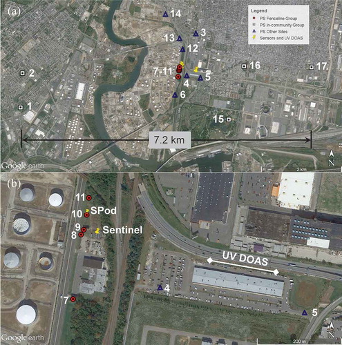
In complex urban airsheds, any air sampling site may be located near a temporary or persistent source of benzene with emissions originating from mobile sources, heating oil, gas stations, residential sources, local industry, and so on. The largest potential source of benzene in the study area is the PES refinery and other industry and tankage located to the west of sites 6–13 (Figure 1). Here, we define two primary PS groups based on proximity to the PES facility with other potential spatial groupings examined elsewhere (Mukerjee et al., 2016). Sites 7–11 (Figure 1b) are spatially close to each other and to the location of the prototype sensors. These sites are located 35 m (±5 m) east of the PES facility along South 26th Street and are defined here as the “fenceline” group. Site 6 (460 m south of site 7) and site 12 (440 m north of site 11) are also along South 26th Street but are not part of this group. Sites 1, 2, 15, 16, and 17 are located in neighborhoods and are the farthest removed (>1 km) from the PES refinery and other facilities, and are referred to as the “in-community” group.

Passive samplers

Deployments of PSs began on June 18, 2013, and concluded on March 25, 2015, producing a total of 41 valid sampling periods with 655 total PS results after duplicate averaging. The nominal duration of each sampling period was 14 d. Due to resource constraints, sampling periods 5 and 12 were extended in duration (20 d and 29 d, respectively), and several deployment weeks were skipped during the October 2013 U.S. government shutdown. Sampling period 7 was invalidated due to instrument malfunction during analysis.

The diffusive tube PSs used in this study, along with protective housings, are shown in Supplemental Figure S2. The PSs were 89 mm long, 6.4 mm outer diameter stainless-steel tubes, part number 28686-U, Supelco FLM Carbopack X deactivated TD tube for fenceline monitoring (Sigma-Aldrich, St. Louis MO), with 6.4-mm brass Swagelok endcaps, one-piece Teflon ferrules, and part number L4070207 diffusion caps (PerkinElmer, Shelton, CT). Prior to deployment, the PSs were conditioned in the laboratory at 350°C for 1 hr while purging with nominally 75 mL/min of helium and shipped to the site along with field blanks and field spikes in a cooler (no ice) to provide some thermal stability and physical protection. Following deployment documentation, the brass endcap on the sampling end of a PS was removed and replaced with a diffusion cap (Figure S2a) to expose the sorbent to ambient air. The PS was mounted in a protective housing using a snap-in aluminum holder; then the housing was secured to a structure at the site. After nominally 14 d of exposure, the PS was capped, registered on a chain-of-custody document, packaged, and shipped in a cooler to the EPA Office of Research and Development (ORD) laboratory for analysis. Upon receipt in the laboratory and prior to analysis, the sample tubes were refrigerated. Analysis was by thermal desorption gas chromatography/mass spectrometry (GC/MS) using a modified version of U.S. EPA Method 325B (EPA, 2015c). A correction procedure was used to remove the measured benzene artifacts on the sorbent, and additional procedures corrected for drift in instrument calibration response.

The field change-outs of the PS sets typically required 6 hr and were executed between the hours of 7:00 a.m. and 1:00 p.m. When a set of PSs was retrieved, a new unexposed set was usually deployed. In most cases, multiple PSs were deployed in a single housing at a given location for duplicate, field blank, and field spike quality control purposes. A group of three PSs with diffusion caps installed in a protective housing are shown in Supplemental Figure S2b along with two types of mounting systems (Figure S2c and S2d). The housings were designed to install easily at the site by clipping onto existing structures (such as a fence) or by hanging on previously installed hook-like fixtures. For deployments in communities, the PSs were attached to light poles ~3.7 m above the ground to minimize tampering. For these sites, the “hanging type” housing (Figures S2b and S2c) was employed and the operator used a 3-m pole to set and retrieve the housings.

General information on EPA’s use of Carbopack X diffusive tube PSs for near-source and personal exposure applications along with field comparisons to automated gas chromatograph and canister measurements for 1- or 2-wk deployments can be found in the literature (McClenny et al., 2005; Mukerjee et al., 2009; Thoma et al., 2011). This project used duplicates, field blanks, and field spikes as primary quality control checks and was executed as part of a larger effort that deployed PS in several areas of the United States (Eisele et al., 2016; Mukerjee et al., 2016; Thoma et al., 2015). For the Philadelphia deployment, in total 1264 individual PS results, yielding 609 duplicate pairs, passed quality assurance checks and are part of this analysis. Duplicate comparisons for benzene indicated good precision with an average percent difference of 1.5% and a maximum of 34%, with 13 of 609 values exceeding 10% difference (Figure 2). After correction for benzene artifact (average [avg.] ~0.04 ppbv ± 0.02 ppbv) on all tubes, the mean for the field blanks was 0.005 ± 0.146 ppbv (N = 135). The field spike recoveries were 100.1 ± 9.6% (N = 136). The method detection limit for the set was below 0.02 ppbv in all cases. All values are based a 14-d tube exposure. Future publications will investigate PS performance for multiple compounds under different climatic and siting conditions and will compare other sampling methods and analyses performed by multiple laboratories. For subsequent discussion, co-deployed field and duplicate samples were averaged where available to produce a single value yielding 655 individual PS readings for the study.

Fenceline sensors

Time-resolved measurement of air pollutant and wind data at the facility fencelines can detect emissions and help determine their origin. Reflecting a wide spectrum of performance and implementation costs, time-resolved fenceline measurement approaches can range from high performance open-path optical spectroscopy and gas chromatography systems to lower cost “leak detection” sensors. The two-unit prototype sensor network used in this study (Supplemental Figure S3) investigates the low end of the cost and performance spectrum. The two sensor nodes, called SPod and Sentinel, are based on passive (nonpumped) photoionization detectors (PIDs, blue label piD-TECH eVx, Baseline-Mocon, Inc., Lyons, CO), and provided an uncalibrated measure of VOC and HAP compounds that are ionized by the 10.6-eV lamp, which includes benzene, toluene, ethylbenzene, and xylenes (BTEX). The systems used an EPA-developed sensor board (Figure S3a inset) supporting the PID and the following additional sensors: relative humidity (HIH-4030, Honeywell, Morristown, NJ); atmospheric pressure (MPX4115AP, Freescale Semiconductor, Tempe, AZ); and atmospheric temperature (MCP9700A, Microchip Technology, Chandler, AZ). The solar-powered SPod (Figure S3a) was controlled by a low-cost and low-power-consumption Arduino MEGA computer and communicated with the Sentinel base station (Figure S3b) using a short-range ZigBee (IEEE 802.15.4) network. The Sentinel base station was fitted with a model 81000V ultrasonic anemometer (R.M. Young, Inc., Traverse City, MI) for wind measurements and communicated via a cellphone modem using a custom data acquisition program. Both units log time-synchronized data at 1 Hz, and an amplification gain of 40× is used on the PID signal for this study.

For these low-cost sensor systems, no attempt was made to condition the air presented to the PID sensors or to stabilize their temperatures. As a consequence, the output signal of the PID exhibits a slowly varying baseline drift (minutes to hours) due both to instrument effects and to changes in the background air mass. When observed from a fixed single point fenceline location, the wind-advected plume from a proximate emission source produces a rapidly changing time-dependent concentration signal (seconds) that can be decoupled from the slowly varying baseline drift through a spline fit. Supplemental Figure Set S5 illustrates the baseline correction process and shows PID sensor data for PS sampling period 34 (discussed subsequently) and indicates time periods where the sensors were offline. Sensor malfunctions were caused primarily by nonoptimized signal amplification, which has been corrected in later versions. Further information on EPA fenceline sensors is contained in the literature (Jiao et al., 2015; Thoma et al., 2015).

Open-path optical systems

As part of a 2011 EPA Community-Scale Air Toxics Monitoring Grant, AMS deployed an open-path ultraviolet differential optical absorption spectrometer (UV DOAS, deuterium lamp model 2012, Cerex Environmental Solutions, Atlanta, GA) and an open-path hydrogen fluoride infrared tunable diode laser (Spectra-1, PKL Technologies Inc., Edmonton, AB, Canada). Both systems were monostatic in configuration with the source/receiver and retroreflectors at east site and west sites, respectively (Figure 1b), and were attached to elevated platforms using shipping containers producing optical beams ~4 m above ground level (Supplemental Figure S4). The optical path lengths (double pass) were 323 m with center points located ~430 m due east of the PES fenceline. The UV DOAS, the only system described here, operated with a 5-min time resolution, integrating on the order of 1700 individual spectral acquisitions during each period.

To meet AMS’s overall project goals, the UV DOAS was configured to simultaneously measure multiple HAPs and criteria pollutants, so the benzene-specific measurement performance is somewhat reduced compared to current commercially available units optimized for that purpose (Thoma et al., 2016). The method detecton limit (MDL) is defined here as meeting both minimum signal-to-noise ratio (SNR) and minimum spectral correlation coefficent (R²) requirements. For detection, the benzene signal determined must exceed three times the standard deviation in noise measured in a 275-nm to 276-nm window (otherwise stated, SNR > 3σ). Additionally, the R² of the scaled benzene reference and field spectra must exceed 0.70 (Supplemental Figures S6 and S7). The MDL of the UV DOAS for benzene in the present analysis study is typically 2–3 ppbv under good conditions.

Results and discussion

Passive sampler summary

Table 1 summarizes the period mean, minimum, and maximum benzene concentrations for all sites, in addition to the mean values for the in-community (0.29 ppbv) and fenceline groups (1.22 ppbv). Using a Wilcoxon–Mann–Whitney test, the differences in means for the fenceline and in-community groups are statistically significant at the 95% confidence level (p < 0.001). The maximum period benzene reading (5.02 ppbv) occurred at fenceline group site 8. The overall study mean (0.70 ppbv) was determined in part by the relative number of near fenceline (source-proximate) and remote sites. As a point of comparison, PS site 3 was located ~450 m from the nearest facility fenceline at the AMS Ritner Avenue Air Quality Monitoring station and recorded a study mean benzene concentration of 0.42 ppbv (σ = 0.10 ppbv). As part of standard operations, the AMS station performed EPA Compendium Method TO-15 “1 in 6 day” whole air canister sampling. Excluding two readings that were below the detection limit, the canister-derived mean benzene concentration at site 3 over the study period was 0.32 ppbv (σ = 0.23 ppbv, N = 104).

Table 1. Summary of passive sampler benzene data by period (before background subtraction).

Sampling period number	Period midpoint (mm/dd/yy)	All sites mean (ppbv)	All sites minimum (ppbv)	Location of period minimum	All sites maximum (ppbv)	Location of period maximum	In-community group mean (ppbv)	Fenceline group mean (ppbv)
1	06/25/13	0.42	0.18	1	0.80	13	0.24	0.51
2	07/16/13	1.12	0.15	1	2.74	9	0.20	2.47
3	07/30/13	0.99	0.22	1	3.13	8,9	0.25	2.17
4	08/14/13	1.14	0.18	2	3.05	8	0.25	2.50
5	08/31/13	0.70	0.19	1	1.64	8	0.22	1.33
6	09/17/13	0.60	0.17	1	1.65	7	0.19	1.27
8	10/29/13	0.45	0.24	2	0.95	9	0.25	0.76
9	11/13/13	0.68	0.22	1	1.53	9	0.24	1.29
10	11/27/13	0.66	0.32	2	1.67	9	0.35	1.16
11	12/11/13	0.56	0.33	2	0.93	8	0.37	0.81
12	01/02/14	0.57	0.31	15	0.90	9	0.32	0.79
13	01/22/14	0.58	0.31	2	0.99	9	0.34	0.82
14	02/04/14	1.09	0.65	14	1.67	6	0.69	1.36
15	02/19/14	1.16	0.44	14	2.95	8	0.57	1.97
16	03/04/14	0.88	0.34	15	2.06	8	0.40	1.57
17	03/18/14	0.85	0.27	2	2.39	8	0.31	1.74
18	04/01/14	0.93	0.29	17	2.31	8	0.41	1.69
19	04/15/14	0.76	0.23	17	1.48	8	0.25	1.27
20	04/29/14	1.02	0.20	17	2.89	8	0.28	2.23
21	05/13/14	0.54	0.19	17	1.16	8	0.24	0.94
22	05/27/14	0.70	0.19	1	1.65	8	0.19	1.41
23	06/10/14	0.56	0.18	15	1.50	8	0.20	1.06
24	06/25/14	0.40	0.08	15	1.24	8	0.13	0.80
25	07/09/14	0.70	0.13	2	1.63	12	0.15	1.27
26	07/23/14	0.55	0.19	15	1.08	8	0.20	0.91
27	08/05/14	0.49	0.15	12	1.86	8	0.20	1.03
28	08/19/14	0.58	0.20	2	1.40	8	0.24	1.04
29	09/02/14	0.69	0.19	15	1.33	8	0.20	1.20
30	09/16/14	0.46	0.21	17	0.98	8	0.25	0.77
31	09/30/14	0.43	0.22	15	0.65	12	0.27	0.59
32	10/14/14	0.45	0.22	1	0.65	8	0.23	0.60
33	10/28/14	0.61	0.22	2	1.05	8	0.25	0.95
34	11/11/14	1.36	0.30	17	5.02	8	0.32	3.11
35	11/26/14	0.58	0.26	17	1.10	9	0.29	0.89
36	12/09/14	0.42	0.31	14	0.54	7	0.34	0.52
37	12/23/14	0.47	0.29	17	0.67	8	0.32	0.61
38	01/21/15	0.58	0.30	14	1.01	8	0.40	0.83
39	02/04/15	0.55	0.35	2	0.76	7	0.40	0.65
40	02/17/15	0.79	0.42	2	1.35	7	0.48	1.16
41	03/03/15	0.79	0.31	1	1.27	12	0.35	1.13
42	03/17/15	0.65	0.29	1,17	1.54	6	0.31	0.85
Average	N/A	0.70	0.25	N/A	1.59	N/A	0.29	1.22
Median	N/A	0.61	0.22	N/A	1.40	N/A	0.25	1.06
Std. dev.	N/A	0.24	0.10	N/A	0.89	N/A	0.11	0.60
Minimum	N/A	0.40	0.08	N/A	0.54	N/A	0.13	0.51
Maximum	N/A	1.36	0.65	N/A	5.02	N/A	0.69	3.11

Table 1 also shows the site locations where the minimum and maximum benzene concentrations were recorded for each sampling period. The location of the period minimum was part of the in-community group in 36 of 41 cases with results from multiple sites usually within <0.1 ppbv.

The maximum period concentration was part of the fenceline group in 35 of 41 cases with the other cases occurring at sites located close to the facility fenceline (e.g., sites 6 and 12) but not part of the defined group. Overall, the presence of ~1 ppbv elevated benzene concentrations at a refinery fenceline is not unexpected, and if indicative of whole-facility values, would not require corrective action under the recently promulgated work practice (EPA, 2015a).

Time-integrated PSs in fenceline and community applications provide average pollutant concentration data acquired over a mixture of source emission and atmospheric states. The meteorological conditions for this study by sampling period are summarized in Supplemental Table ST1. The prevailing wind was from the west, as evidenced by the consistently positive east component of the resultant wind vector. The northerly wind component was mixed with winds tending to be from the north in wintertime periods. Four wintertime minimum period concentrations were recorded at site location 14, located ~750 m north of the PES refinery. Minimum period benzene concentrations were elevated in the winter months (Table 1 and Figure 3a). This elevation is further explored in Figure 3b, which plots the minimum period concentrations versus average period temperature. The variability in minimum period concentrations is likely due to a combination of seasonal source factors (e.g., mobile source fuel mix, cold starts, heating, etc.), atmospheric factors (mixing layer height and inversions), and potential environmental effects on PS performance characteristics.

Figure 2. PS duplicate comparisons for this study (N = 609 pairs).

Figure 3. (a) Minimum PS value by sample period, and (b) average period temperature.

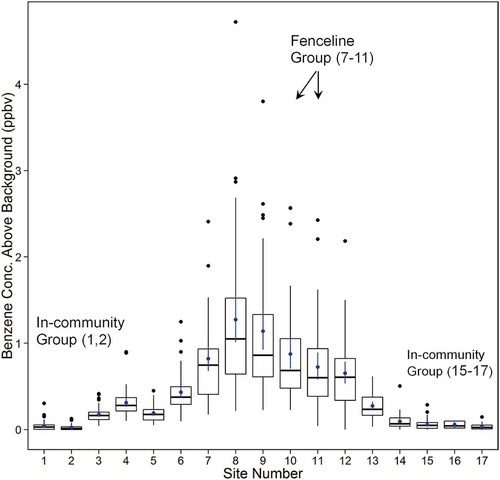
In subsequent discussion, the minimum PS concentration for each sampling period was designated as the ambient benzene background and subtracted from the measured benzene concentrations at the remaining sites (similar to Method 325A and B). This background subtraction can assist in comparing results across sites and sampling periods but should not be used for absolute ambient level comparisons and may reduce the impact of air shed sources in spatial analyses. Figure 4 summarizes background-subtracted PS concentration data across all periods by sampling location. It is evident that the in-community sites (1, 2, 15–17) show consistently low benzene concentrations in comparison to the fenceline group (7–11). The fenceline sites are close to the PES refinery but they are also along a road with significant traffic volume and near other potential industrial sources. An argument against significant roadway contribution to the fenceline signal is found by comparing the fenceline group to sites 6 and 12, also along South 26th Avenue with similar traffic volumes. Additionally, sites 13 and 14 are near major roadways but are not significantly elevated in comparison to the fenceline group. The lack of rush-hour signal on the sensors along South 26th further supports this point (Supplemental Figure Set S5). Taken together, these points indicate that mobile source-generated benzene signal is not likely to be the most significant contributing factor for elevated readings within the fenceline group.

Figure 4. PS benzene data by site, combining all sampling periods. The box whiskers extend to the largest measurement <1.5 times the interquartile range. Blue markers indicate means with 95% confidence intervals calculated by nonparametric bootstrap.

Temporal and spatial variability

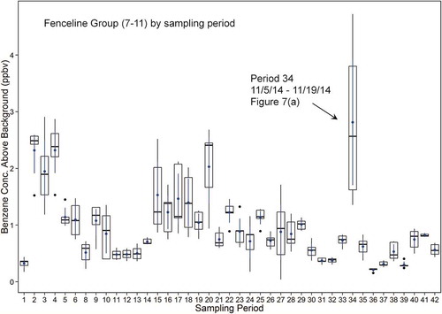
With background-subtracted mean concentrations ranging from 0.21 ppbv (Period 36) to 2.81 ppbv (Period 34), the fenceline group exhibits significant variability (Figure 5). A portion of this variability is likely to be due to changes in nearby source emissions and part is due to changes in atmospheric conditions over time, but it is clear that local sources are present. Period 34 (November 5–November 19, 2014) is sharply elevated compared to neighboring periods under similar meteorological conditions (Supplemental Table ST1), with the exception of a higher percentage of wind speed lulls (13% in Period 34 vs. 2–3%). Although the fenceline group sites are located relatively close to each other (within 240 m; Figure 1b) compared to overall facility fenceline length, the fenceline group sites showed somewhat different responses. The highest benzene readings were consistently observed at sites 8 and 9, spatially separated ~13 m, with these sites driving the overall fenceline group averages and responsible for the high outlier values of Figure 4. These differences may point to a proximate source for sites 8 and 9, but these sites also have the least amount of nearby wind flow obstructions in the fenceline group. The trees and topography directly behind sites 6–12 affect wind flow from certain directions (and therefore registered concentrations) in complex ways. These effects may include channeling of signal along 26th Street or urban canyon-like effects that could increase or decrease concentrations compared to the optimal free-flowing case.

Figure 5. PS benzene data for the fenceline group by sampling period. The box whiskers extend to the largest measurement <1.5 times the interquartile range. Blue markers indicate means with 95% confidence intervals calculated by nonparametric bootstrap.

Spatial variability was investigated by plotting the PS benzene concentration data by site as a function of distance from the nearest facility fenceline (Figure 6a). Three regimes are evident with sites 6–12 within 50 m of a fenceline, sites 13, 4, 3, 5, and 14 between 150 m and 750 m from a fenceline, and the in-community sites at distances >1 km. A general gradient in concentrations is evident with sites 1 and 2 on the predominately upwind side and sites 13 and 14 with positions offset to the north showing somewhat lower relative response, as may be expected under an overall resultant wind vector, –0.4 m/sec north, 1.3 m/sec east (Supplemental Table ST1). As shown in Figure 1b, sites 4 and 5 are due east of the fenceline group and show elevated but decreasing concentrations, as would be expected from a source to the west. When considering this gradient, the observed benzene levels at sites 4 and 5 are also likely to be affected by the trees and topography that separate these locations from the fenceline group.

Figure 6. (a) PS benzene site means for all sampling periods vs. distance from nearest facility fenceline with site locations noted, and (b) gradient formed by the fenceline group and sites 4 and 5 for all sampling periods and for Period 34. Error bars indicate 95% confidence interval for means calculated by nonparametric bootstrap.

Figure 6b further examines the gradient in concentration formed by the fenceline group and sites 4 and 5 for all periods and for Period 34 when the highest readings were observed. A comparison of the fenceline groups and the site 4 groups in Figure 6b indicate an approximate factor of three difference in benzene concentrations in Period 34. The ratio of concentrations at site 5 is somewhat lower, but this low ratio may be due to the direction of plume transport during Period 34, further discussed in the following. Additional information on the origins of emissions and the subsequent informed analysis of the concentration gradients is the subject of future work.

Time-resolved measurements

Time-resolved pollutant concentration and wind field measurements can help inform time-integrated PS data acquired over a mixture of meteorological conditions. As an example, consider UV DOAS and wind data for outlier Period 34 (Figures 7 and 8). Figure 7a shows 5-min average PID readings for the SPod and Sentinel sensors along with UV DOAS benzene concentration measurements for the 2-wk period. The sensors were off-line, as noted with further details in Supplemental Figure Set 5. The sensors show strong signal response indicative of emission plumes from the west on November 5, 2014, and November 15, 2014. Using an MDL definition of SNR > 3σ and R² > 0.70, the UV DOAS registered 35 in-detection benzene events for 5-min averages during Period 34, with more than half of these occurring on November 15, 2014. Increasing the MDL R² requirement to >0.80 reduces the number of in-detection events to 9, with all but one of these occurring on November 15, 2014. An example of the benzene spectra acquired and the reference is contained in Supplemental Figure S7.

Figure 7. (a) Sensor and UV DOAS data for entire PS Period 34 (11/5/14–11/19/14) and (b) same from 12:00 a.m. on 11/15/14 to 12:00 p.m. on 11/16/14. Due to clock drift, there is an uncertainty (likely <1 hr) in the synchronization systems.

Figure 8. (a) Wind direction and speed from Sentinel Sensor from 12:00 a.m. on 11/15/14 to 12:00 p.m. on 11/16/14, and (b) SPod and Sentinel sensor responses (color bar) as function of wind direction and wind speed 11/15/14 12:00 a.m. to 12:00 p.m.

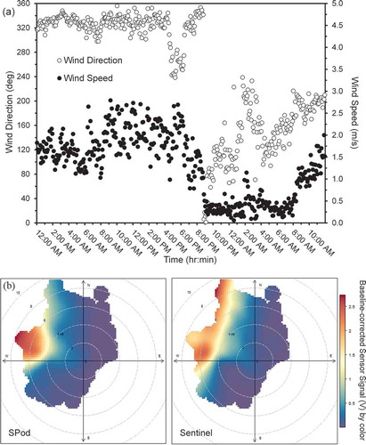
Figure 7b shows an expanded view from 12:00 a.m. on November 15, 2014, to 12:00 p.m. on November 16, 2014. Two primary events can be identified. The largest sensor signal (full scale) and UV DOAS benzene reading (24 ppbv) were obtained around noon on November 15, 2014. Significant sustained response on the UV DOAS was also observed at approximately midnight on November 15, 2014. The sensor signal at this latter time was also present but is underestimated by approximately 1 V due to nonoptimal automated background subtraction caused by the slowly varying air mass. Figure 8a shows wind speed and direction acquired by the Sentinel sensor over the same 36-hr time period, and Figure 8b presents the SPod and Sentinel sensor responses (color bar) as function of wind direction and wind speed for November 15, 2014. The noon November 15, 2014, signal is obtained under relatively constant 2-m/sec wind from the northwest. A proximate source from the facility is evident from Figure 8b. The narrower directionality in the SPod signal compared to the Sentinel is ascribed to the location of the former in a more open area with less potential wind flow obstructions and backing topography (Figure 1b). In the evening of November 15, 2014, the wind speed decreases dramatically, and the wind direction shifts, creating a stagnant air mass, which when potentially coupled with a compressing boundary layer results in a sustained 5–10 ppbv benzene level registered by UV DOAS. The second event is more difficult to see with the sensor systems geared to fast proximate plume detection. It is important to note that the latter sustained benzene levels may be due to a mixture of sources. Taken together, it appears that the majority of the PS signal for period 34 may be associated with these discrete multihour events.

Summary

An overview of the Philadelphia Passive Sampler and Sensor Study was provided, and PS benzene results were summarized. Analysis of co-deployed duplicate pairs indicated relatively robust precision performance, and a negative correlation between the period minimum benzene concentrations and average temperature was observed. The overall mean concentration for a group of in-community sites was 0.29 ppbv. Benzene concentrations for PSs located in proximity to facility fencelines were consistently elevated, with an overall average ~1 ppbv higher than the in-community sites. An example of time-resolved data to inform the PS results was provided and indicated that much of the signal recorded by the PS during the 2-wk sampling period with the highest benzene levels is likely to be due to a few discrete multihour events. An examination of prevailing winds, spatial gradients in concentration, and an example of time-resolved data from Period 34 support the notion of benzene sources to the west of sites 7–11.

Building on this overview paper, additional analysis from the study will explore topics such as fenceline sensor data, additional chemical species, source transport modeling, and exposure levels. As a preliminary conclusion, 2-wk PS (variation of Method 325A and B) can be successfully deployed near sources and in communities to provide valuable long-term, geospatially resolved air quality data. When used in conjunction with time-resolved sensor systems, PS can help improve information on air pollutant concentrations in areas with many potential sources (like South Philadelphia).

Funding

The authors thank EPA colleagues Dave Nash, and Wan Jiao, now with ICF International, for development of the prototype fenceline sensors used in this study. This work would not have been possible without the efforts of EPA’s Maribel Colon, John Turlington, and Lillian Alston (EPA SEE program) on PS laboratory and data analysis. We thank EPA colleagues Jason DeWees, Ray Merrill, Brenda Shine, Ken Garing, Edgar Thompson, Adam Eisele, and Ron Landy for ongoing collaboration on these topics. Thanks to Mark Modrak, now with AECOM, and Shahrooz Amin, now with Industrial Monitoring and Control Corporation, for their efforts on this project. Thanks to Tom Wisniewski, Scott McEwan, and Paul Johnson with Cerex Environmental Solutions for data analysis assistance. Funding for the PS and sensor portion of the study was provided by U.S. EPA ORD’s Air, Climate, and Energy (ACE) and Regional Applied Research Effort (RARE) programs. The AMS open-path deployment was funded under EPA’s Community-Scale Air Toxics Ambient Monitoring Grant Program (EPA-OAR-OAQPS-11-05; 96311601-1). The views expressed in this article are those of the authors and do not necessarily represent the views or policies of the U.S. Environmental Protection Agency. Mention of any products or trade names does not constitute endorsement.

Supplemental data

Supplemental data for this paper can be accessed at the publisher’s website.

Additional information

Funding

The authors thank EPA colleagues Dave Nash, and Wan Jiao, now with ICF International, for development of the prototype fenceline sensors used in this study. This work would not have been possible without the efforts of EPA’s Maribel Colon, John Turlington, and Lillian Alston (EPA SEE program) on PS laboratory and data analysis. We thank EPA colleagues Jason DeWees, Ray Merrill, Brenda Shine, Ken Garing, Edgar Thompson, Adam Eisele, and Ron Landy for ongoing collaboration on these topics. Thanks to Mark Modrak, now with AECOM, and Shahrooz Amin, now with Industrial Monitoring and Control Corporation, for their efforts on this project. Thanks to Tom Wisniewski, Scott McEwan, and Paul Johnson with Cerex Environmental Solutions for data analysis assistance. Funding for the PS and sensor portion of the study was provided by U.S. EPA ORD’s Air, Climate, and Energy (ACE) and Regional Applied Research Effort (RARE) programs. The AMS open-path deployment was funded under EPA’s Community-Scale Air Toxics Ambient Monitoring Grant Program (EPA-OAR-OAQPS-11-05; 96311601-1). The views expressed in this article are those of the authors and do not necessarily represent the views or policies of the U.S. Environmental Protection Agency. Mention of any products or trade names does not constitute endorsement.

Notes on contributors

Eben D. Thoma

Eben D. Thoma and Tai Wu are Physical Scientists, Bill Mitchell is a Technical Specialist, and Halley L. Brantley is an ORISE Fellow with EPA’s Office of Research & Development (ORD), National Risk Managment Research Laboratory.

Halley L. Brantley

Eben D. Thoma and Tai Wu are Physical Scientists, Bill Mitchell is a Technical Specialist, and Halley L. Brantley is an ORISE Fellow with EPA’s Office of Research & Development (ORD), National Risk Managment Research Laboratory.

Karen D. Oliver

Karen D. Oliver is a Research Chemist and Shaibal Mukerjee and Donald A. Whitaker are Research Physical Scientists with EPA’s Office of Research & Development (ORD), National Exposure Research Laboratory (NERL).

Donald A. Whitaker

Karen D. Oliver is a Research Chemist and Shaibal Mukerjee and Donald A. Whitaker are Research Physical Scientists with EPA’s Office of Research & Development (ORD), National Exposure Research Laboratory (NERL).

Shaibal Mukerjee

Karen D. Oliver is a Research Chemist and Shaibal Mukerjee and Donald A. Whitaker are Research Physical Scientists with EPA’s Office of Research & Development (ORD), National Exposure Research Laboratory (NERL).

Bill Mitchell

Eben D. Thoma and Tai Wu are Physical Scientists, Bill Mitchell is a Technical Specialist, and Halley L. Brantley is an ORISE Fellow with EPA’s Office of Research & Development (ORD), National Risk Managment Research Laboratory.

Tai Wu

Eben D. Thoma and Tai Wu are Physical Scientists, Bill Mitchell is a Technical Specialist, and Halley L. Brantley is an ORISE Fellow with EPA’s Office of Research & Development (ORD), National Risk Managment Research Laboratory.

Bill Squier

Bill Squier is a Mechanical Engineer with EPA’s Office of Enforcement and Compliance Assurance, National Environmental Investigations Center.

Elsy Escobar

Elsy Escobar is an Environmental Engineer 2 with Arcadis U.S.

Tamira A. Cousett

Tamira A. Couset is a Chemist with Jacobs Technology.

Carol Ann Gross-Davis

Carol Ann Gross-Davis, PhD, is an Epidemiologist and Howard Schmidt is a Scientist with EPA Region 3, Air Protection Division.

Howard Schmidt

Carol Ann Gross-Davis, PhD, is an Epidemiologist and Howard Schmidt is a Scientist with EPA Region 3, Air Protection Division.

Dennis Sosna

Dennis Sosna is an Administrative Scientist and Hallie Weiss is an Administrative Engineer with the City of Philadelphia, Department of Public Health, Air Management Services Laboratory.

Hallie Weiss

Dennis Sosna is an Administrative Scientist and Hallie Weiss is an Administrative Engineer with the City of Philadelphia, Department of Public Health, Air Management Services Laboratory.

References

- Brantley, H.L., E.D. Thoma, W.C. Squier, B.B. Guven, and D. Lyon. 2014. Assessment of methane emissions from oil and gas production pads using mobile measurements. Environ. Sci. Technol. 48(24):14508–15. doi:10.1021/es503070q
- Eisele, A.P., S. Mukerjee, L.A. Smith, E.D. Thoma, D. Whitaker, K. Oliver, T. Wu, M. Colon, L. Alston, T. Cousett, M.C. Miller, D.M. Smith, and C. Stallings. 2016. Volatile organic compounds at oil and natural gas production well pads in Colorado and Texas using passive samplers. J. Air Waste Manage. Assoc. 66( 4):412–19. doi:10.1080/10962247.2016.1141808.
- EPA, U.S. 2015a. Petroleum refinery sector risk and technology review and new source performance standards—Final rule. Fed. Reg. 40 CFR Part 63, ID: EPA-HQ-OAR-2010-0682-0700. https://www.regulations.gov (accessed March 24, 2016).
- EPA, U.S. 2015b. Method 325A—Volatile Organic Compounds from Fugitive and Area Sources: Sampler Deployment and VOC Sample Collection. 40 CFR Part 63, Subpart UUU, Appendix A [EPA-HQ-OAR-2010-0682-700], Petroleum Refinery Sector Risk and Technology Review and New Source Performance Standards. https://www.regulations.gov (accessed March 24, 2016).
- EPA, U.S. 2015c. Method 325B—Volatile Organic Compounds from Fugitive and Area Sources: Sampler Preparation and Analysis. 40 CFR Part 63, Subpart UUU, Appendix A [EPA-HQ-OAR-2010-0682-700], Petroleum Refinery Sector Risk and Technology Review and New Source Performance Standards. https://www.regulations.gov (accessed March 24, 2016).
- Jiao, W., E.D. Thoma, E. Escobar, M. Modrak, S. Amin, B Squier, and B. Mitchell. 2015. Investigation of a low cost sensor-based leak detection system for fence line applications. Proceedings of the 108th Annual Conference of the Air & Waste Management Association, June 23–26, 2015, Raleigh, NC. http://www.awma.org/events-webinars/past-event-proceedings/category?Id=63 ( accessed March 24, 2016).
- Marchese, A.J., T.L. Vaughn, D.J. Zimmerle, D.M. Martinez, L.L. Williams, A.L. Robinson, A.L. Mitchell, R. Subramanian, D.S. Tkacik, J.R. Roscioli, and S.C. Herndon. 2015. Methane emissions from United States natural gas gathering and processing. Environ. Sci. Technol. 49(17): 10718–27. doi: 10.1021/acs.est.5b02275
- McClenny, W.A., K.D. Oliver, H.H. Jacumin, E.H. Daughtrey, and D.A. Whitaker. 2005. 24 H diffusive sampling of toxic VOCs in air onto Carbopack X solid adsorbent followed by thermal desorption/GC/MS analysis-laboratory studies. J. Environ. Monit. 7(3): 248–56. doi:10.1039/B412213E
- Mellqvist, J., J. Samuelsson, J. Johansson, C. Rivera, B. Lefer, S. Alvarez, and J. Jolly. 2010. Measurements of industrial emissions of alkenes in Texas using the solar occultation flux method. J. Geophys. Res. Atmos. 115:D00F17. doi:10.1029/2008JD011682
- Mukerjee, S., L. Smith, E.D. Thoma, K. Oliver, D. Whitaker, T. Wu, M. Colon, L. Alston, T. Cousett, and C. Stallings. 2016. Spatial analysis of volatile organic compounds in South Philadelphia using passive samplers. J. Air Waste Manage. Assoc. in press. doi:10.1080/10962247.2016.1147505
- Mukerjee, S., K.D. Oliver, R.L.Seila, H.H. Jacumin, Jr., C. Croghan, E,H. Daughtrey, Jr., L.M. Neas, and L.A. Smith. 2009. Field comparison of passive air samplers with reference monitors for ambient volatile organic compounds and nitrogen dioxide under week-long integrals. J. Environ. Monit. 11(1): 220–27. doi:10.1039/B809588D
- Olaguer, E.P., M.H. Erickson, A. Wijesinghe, and B.S. Neish. 2015. Source attribution and quantification of benzene event emissions in a Houston ship shannel community based on real time mobile monitoring of ambient air. J. Air Waste Manage. Assoc. 66(2): 164–72. doi: 10.1080/10962247.2015.1081652
- Robinson, R., T. Gardiner, F. Innocenti, P. Woods, and M. Coleman. 2011. Infrared differential absorption Lidar (DIAL) measurements of hydrocarbon emissions. J. Environ. Monit. 13(8): 2213–20. doi:10.1039/c0em00312c
- Snyder, E.G, T.H. Watkins, P.A. Solomon, E.D. Thoma, R.W. Williams, G.S.W. Hagler, D. Shelow, D.A. Hindin, V.J. Kilaru, and P.W. Preuss. 2013. The changing paradigm of air pollution monitoring. Environ. Sci. Technol. 47(20): 11369–77. doi:10.1021/es4022602
- Thoma, E.D., M.C. Miller, K.C. Chung, N.L. Parsons, and B.C. Shine. 2011. Facility fenceline monitoring using passive samplers. J. Air Waste Manage. Assoc. 61(8): 834–42. doi:10.3155/1047-3289.61.8.834
- Thoma, E.D., W Jiao, H. Brantley, T. Wu, B. Squier, B. Mitchell, K. Oliver, D. Whitaker, S. Mukerjee, M. Colon, L. Alston, C.A. Gross-Davis, H. Schmidt, R. Landy, J. DeWees, R. Merrill, E. Escobar, M.S. Amin, and M. Modrak. 2015. South Philadelphia passive sampler and sensor study: interim report. Proceedings of the 108th Annual Conference of the Air & Waste Management Association, June 23–26, 2015, Raleigh, NC. http://www.awma.org/events-webinars/past-event-proceedings/category?Id=63 ( accessed March 24, 2016).
- Thoma, E.D., E. Thompson, J. DeWees, P. Deshmukh, T. Wisniewski, S. McEwan, P. Johnson, D. Sosna, H. Weiss, C. Gross-Davis, and H. Schmidt. 2016. Testing of a Cerex open-path ultraviolet differential optical absorption spectroscopy systems for fenceline monitoring applications. Proceedings of the Air and Waste Managment Association Air Quality Measurement Methods and Technology, March 15–17, 2015, Chapell Hill, NC. http://www.awma.org/events-webinars/past-event-proceedings (accessed March 24, 2016).
- Wu, C.F., T.G. Wu, R.A. Hashmonay, S.Y. Chang, Y.S. Wu, C.P. Chao, C.P. Hsu, M.J. Chase, and R.H. Kagann. 2014. Measurement of fugitive volatile organic compound emissions from a petrochemical tank farm using open-path Fourier transform infrared spectrometry. Atmos. Environ. 82: 335–42. doi:10.1016/j.atmosenv.2013.10.036
- Zavala-Araiza, D., D. Lyon, R.A. Alvarez, V. Palacios, R. Harriss, X. Lan, R. Talbot, and S.P. Hamburg. 2015. Toward a functional definition of methane super-emitters: application to natural gas production sites. Environ. Sci. Technol. 49(13): 8167–74. doi:10.1021/acs.est.5b00133