Investigating the real-world emission characteristics of light-duty gasoline vehicles and their relationship to local socioeconomic conditions in three communities in Los Angeles, California

ABSTRACT

This paper discusses results from a vehicular emissions research study of over 350 vehicles conducted in three communities in Los Angeles, CA, in 2010 using vehicle chase measurements. The study explores the real-world emission behavior of light-duty gasoline vehicles, characterizes real-world super-emitters in the different regions, and investigates the relationship of on-road vehicle emissions with the socioeconomic status (SES) of the region. The study found that in comparison to a 2007 earlier study in a neighboring community, vehicle emissions for all measured pollutants had experienced a significant reduction over the years, with oxides of nitrogen (NO_X) and black carbon (BC) emissions showing the largest reductions. Mean emission factors of the sampled vehicles in low-SES communities were roughly 2–3 times higher for NO_X, BC, carbon monoxide, and ultrafine particles, and 4–11 times greater for fine particulate matter (PM_2.5) than for vehicles in the high-SES neighborhood. Further analysis indicated that the emission factors of vehicles within a technology group were also higher in low-SES communities compared to similar vehicles in the high-SES community, suggesting that vehicle age alone did not explain the higher vehicular emission in low-SES communities.

Evaluation of the emission factor distribution found that emissions from 12% of the sampled vehicles were greater than five times the mean from all of the sampled fleet, and these vehicles were consequently categorized as “real-world super-emitters.” Low-SES communities had approximately twice as many super-emitters for most of the pollutants as compared to the high-SES community. Vehicle emissions calculated using model-year-specific average fuel consumption assumptions suggested that approximately 5% of the sampled vehicles accounted for nearly half of the total CO, PM_2.5, and UFP emissions, and 15% of the vehicles were responsible for more than half of the total NO_X and BC emissions from the vehicles sampled during the study.

Implications: This study evaluated the real-world emission behavior and super-emitter distribution of light-duty gasoline vehicles in California, and investigated the relationship of on-road vehicle emissions with local socioeconomic conditions. The study observed a significant reduction in vehicle emissions for all measured pollutants when compared to an earlier study in Wilmington, CA, and found a higher prevalence of high-emitting vehicles in low-socioeconomic-status communities. As overall fleet emissions decrease from stringent vehicle emission regulations, a small fraction of the fleet may contribute to a disproportionate share of the overall on-road vehicle emissions. Therefore, this work will have important implications for improving air quality and public health, especially in low-SES communities.

Introduction

Vehicular emissions are well acknowledged as a major source of urban and global air pollution that contributes to a variety of environmental problems including adverse human health impacts and climate change (Ramanathan and Carmichael, 2008; Garshick et al., 2003). Although vehicle emission standards have become more stringent over the past two decades, the 2013 California Almanac of Emissions and Air Quality shows that on-road mobile sources still emit more than 40% of the statewide diesel particulate matter (DPM) emissions and roughly 50% of the statewide nitrogen oxides (NOx) emissions (California Air Resources Board [CARB], 2013). Researchers have also noted that as particulate matter (PM) emissions from diesel engines continue to be reduced, emissions from light-duty gasoline vehicles (LDGV) could become dominant producers of on-road PM emissions due to the enormous disparity in activity levels for light-duty vehicles compared with diesel vehicles, and could contribute an increasingly large fraction of remaining on-road PM emissions (CARB, 2007b). Furthermore, since the real-world emission behavior of vehicles may be significantly different from the standard test cycles, it is important to study the real-world emissions to help improve regional emissions estimates and to devise effective control programs.

Researchers have also shown that vehicular emissions are especially of concern in low-socioeconomic-status (low-SES) communities where exposure to traffic-related pollutants, especially carbon monoxide (CO) and ultrafine particles (UFP), may be larger due to the proximity to traffic (O’Neill et al., 2003). In addition, these low-SES areas are often burdened with more poorly maintained or older vehicles when compared to higher SES areas (Singer and Harley, 2000; Choi et al., 2013), which further exacerbates the air pollution exposures for residents in low-SES regions. Therefore, effective control of high-emitting vehicles can be an important solution for reducing traffic-related air pollution in these areas.

In California, comprehensive regulations and incentive programs continue to reduce vehicle emissions despite increased travel and economic activity. Although overall fleet-average vehicle emissions have declined significantly due to increasingly strict emission standards and improved control technologies, several researchers have suggested that a small, malfunctioning fraction of fleet on the roadway may emit orders of magnitude higher emissions than normal, well-maintained vehicles, and may be responsible for a disproportionately large fraction of overall vehicle emissions (Park et al., 2011; Singer and Harley, 2000, Lawson et al., 1990; Zhang et al., 1995; CARB, 2007b). A case study of California vehicles noted that high-emitting vehicles would account for up to 6% of vehicle population and vehicle miles traveled, yet they will contribute to more than 75% of exhaust and 66% of evaporative emissions in 2030 (Collet et al., 2015). These high-emitting vehicles are often older, or poorly maintained, or have undergone severe tampering (Cadle et al., 1999). As vehicle emissions have become more tightly controlled, it has become increasingly important to identify and control emissions from super-emitters to meet the federal and state air quality standards. Furthermore, a recent study in Pittsburg, PA, found that high-emitting vehicles contributed up to 70% of the near road particle-bound polycyclic aromatic hydrocarbons (PB–PAH), and 30% of the near-road black carbon (BC) concentrations (Tan et al., 2014). These air pollution enhancements and resulting health exposure impacts are of particular concern for residents in low-SES and environmental justice communities.

Vehicle emission factors have been evaluated using various approaches, including remote sensing tests (Zhang et al., 1995), chassis dynamometer studies (Shah et al., 2006), tunnel studies (Kirchstetter et al., 1999), fleet emission studies (Kozawa et al., 2014), and on-road chase studies (Shorter et al., 2005). However, traditional methods for emissions testing of individual vehicles have significant limitations, including high costs (dynamometer experiments), limitation to fleet average emission rates (tunnel studies), limited location and operating conditions (remote sensing technology), and sample contamination from self-pollution (“follower” mobile units). The California Air Resources Board (CARB) Mobile Measurement Platform (MMP) has a demonstrable advantage of using a zero-emission vehicle for on-road emission measurements and the ability to sample individual vehicles under many different operating conditions. A successful application of this technology has been documented by Park et al. (2011), who reported fuel-based emission factors for 143 light-duty gasoline vehicles measured in Wilmington, CA. By utilizing the same platform and emission analysis methods, we were able to compare the regional passenger vehicle emissions trends in Wilmington, and also to measure emissions from on-road LDGVs in different communities to investigate the association of super-emitter emissions with the general socioeconomic conditions of the communities.

This study further expands the previous research done by Park et al. (2011), and was targeted to understand fleet composition and real-world emission characteristics of light-duty vehicles. The primary objectives of this study were to determine the fleet characteristics of light-duty vehicles in various communities with differing socioeconomic conditions, and to determine the occurrence and overall emission contributions of “real-world super-emitters” (hereafter referred to as “super-emitters”) in high- and low-SES areas based on real-world on-road emission measurements.

Methodology

Earlier on-road work by the authors showed that the mobile platform measurements were able to identify individual super-emitters by chasing them under many different real-world operating conditions (Park et al., 2011). This study utilized the same measurement platform to conduct a chase study of individual vehicles to understand the relationship between community socioeconomic status and LDGV fleet emission behavior. The study used a zero-emission electric vehicle (2002 Toyota RAV4 sub-sports utility vehicle) outfitted with several fast-response air quality analyzers as a mobile measurement platform to conduct on-road measurements of vehicle tailpipe emissions. Pollutants measured by the study included a variety of gas-phase pollutants such as nitrogen oxides (NO_X), carbon monoxide (CO), and carbon dioxide (CO₂), as well as particle-phase pollutants such as particulate matter (PM₁₀ and PM_2.5), black carbon (BC), and ultrafine particles (UFP). Instruments were chosen for compact size, high time resolution, proven robust mobile operation, and low power consumption. The recording time resolution of all instruments was 1 sec. The instruments used for on-road measurements are described in Table 1.

Table 1. List of measurements parameters and equipment.

Instrument	Measurement parameter	Measurement method
TSI condensation particle counter, model 3007	UFP concentrations from 10 to 1,000 nm	Optical
TSI FMPS, model 3091	UFP size distribution and count, 5.6–560 nm	Electrical mobility diameter/electrometer
TSI DustTrak, model 8520	PM2.5 mass	Optical
Magee Scientific Aethalometer, AE 42	Black carbon	Optical attenuation
Teledyne API, model 300E	CO	Nondispersive infrared
LI-COR, model LI-820	CO2	Nondispersive infrared
Teledyne API, model 200E	NOX, NO, NO2	Chemiluminescence

The sampling manifold, calibration procedure, and response time of each instrument are described in detail in an earlier paper (Park et al., 2011). A video camera with an audio system (Stalker Vision) was installed on the front seat of the mobile platform to record the traffic conditions and relative distance between a target vehicle and the platform. A portable global positioning system (GPS; Garmin model 76CSx) was used to record the locations, routes, and vehicle speed with 1-sec resolution. In addition, the plate numbers of chased vehicles were noted during on-road measurements to identify the vehicle’s make, model year, fuel type, and registration ZIP code through Department of Motor Vehicles (DMV) registration records. Sampled vehicles were then assigned to the DMV vehicle registration ZIP code to investigate the emission characteristics of the regional fleets.

This research further expands the application of the previous study and includes several notable improvements to advance the state of measurements and analysis. To increase the sampling efficiency, the sampling protocol of chasing a target vehicle was modified to allow for random selection of many different types of target vehicles, and selection of proper time for at least 20 sec when only one target vehicle was in front of the mobile platform without any interference from other vehicles. Vehicles were chosen randomly and were followed by the mobile platform for sufficient duration to assure valid and representative emissions measurements (described in the following sections), with a typical chasing period of 1–5 minutes. The typical distance between the chased vehicle and the mobile platform was maintained at roughly 10–50 m to capture the target exhaust plume adequately. The driving condition and speed of the chased car were determined based on the moment when the optimal exhaust plume was captured. In general, the measurement routes for all three locations included a stop sign, which allowed the vehicle to capture all driving modes, including acceleration, cruising at 25–35 miles per hour, and deceleration to a complete stop.

The vehicle chase locations were also limited to a few city blocks to allow consistent operation conditions for all vehicles. Since this approach captured a longer driving cycle (and not an instantaneous measurement), it also ensured the vehicles were sufficiently warmed up, allowing consistent measurements of hot stabilized emissions from all the sampled vehicles (not influenced by cold start emissions). During each vehicle chase, the video camera recorded vehicles in front of the mobile platform while the researchers logged/recorded their visual observations to cover off-screen events.

Sampling location

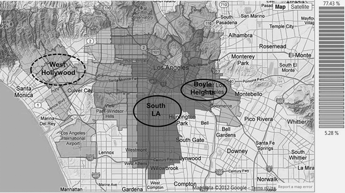
The sampling locations were selected to capture high and low socioeconomic regions in the study area. Data were obtained from the City Data website (City Data Website,n.d.) to identify the population and poverty statistics of different regions, and this information was used to identify regions with different socioeconomic conditions in Los Angeles, CA. Three sampling locations were selected for the study based on the survey: Boyle Heights (with 30% population below the poverty level; L1) and Southeast Los Angeles (38%; L2) were chosen as the low-SES neighborhoods, while West Hollywood (14%; H) was chosen as the high-SES neighborhood, as shown in Figure 1. On-road chase measurements were conducted on small quiet streets enclosed by dense residential areas for three days in each neighborhood during May and June 2010 and exhaust plumes of 131, 121, and 126 LDGVs were collected in the L1, L2, and H neighborhoods, respectively.

Figure 1. Sampling locations showing % population below poverty level (2010).

Data analysis

Fuel-based emission factors were calculated using the carbon balance method based on change in concentrations of a pollutant above the proximal baseline concentrations, measured in the absence of the particular vehicle (eq 1). Emission factor were calculated by normalizing background-subtracted pollutant concentrations to total carbon emitted by the vehicles, and were reported as grams of pollutant per unit kilogram of fuel burned (g/kg):

(1)

where ∆[p] is the background-subtracted concentration of pollutant, μg/m³, and for particle numbers, number/cm³ × 10¹²; ∆[CO2] and ∆[CO] are the average CO₂ and CO concentrations above background, μg/m³; and W_c is the carbon weight fraction (0.85 for gasoline).

More details on the exhaust plume analysis and the calculation of fuel-based emission factors are available in our previous work (Park et al., 2011). Selecting the CO₂ baseline concentration is the major source of uncertainty in calculating the fuel-based emission factors. The baseline of each pollutant for an individual vehicle was selected as the value just before or after the platform encountered a target vehicle and in the absence of other vehicles. Emission factors were calculated only for the vehicles that had no confounding sources prior to and during at least 20 sec of each chase period and that exhibited a 40-ppm increase in CO₂ mixing ratios above the background. The criterion for CO₂ rise was set to ensure an appropriate plume capture and sufficient signal to calculate the emission factors. Valid exhaust plumes were identified for 378 out of 410 LDGVs, and are discussed in this paper in further detail later.

The emission factors were analyzed against their vehicle make and model year information (obtained from DMV vehicle registration data), and vehicle odometer data for accrued vehicle miles traveled (VMT; obtained from California Bureau of Automotive Repair [BAR] Smog Check database). This information was also used to estimate their annual emissions by multiplying the emission factors (g/kg fuel) against the fuel consumption estimates (gallon/vehicle/yr) extracted from California’s Mobile Source Emissions Inventory model (EMFAC2011) by model year and vehicle type (passenger car vs. truck) for Los Angeles county.

Results and discussion

Characteristics of the sampled vehicles

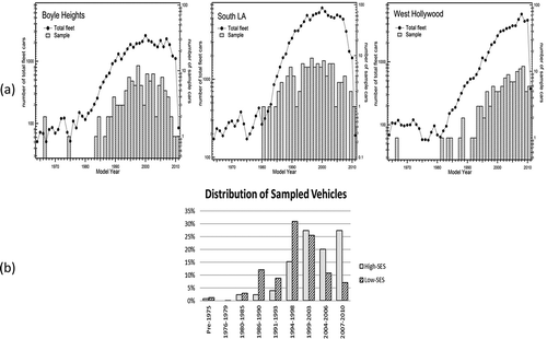
The sampled fleet was first compared against the DMV records to evaluate the representativeness of the fleet in the region. Among the sampled fleet of 378, 15 vehicles did not have any DMV records. The remaining 363 vehicles were classified by city, and each group was analyzed to study the vehicle age distribution (Figure 2). In general, there was good agreement between the sampled vehicles and the DMV registrations. Furthermore, the data also showed that the average model year of the vehicles in high-SES neighborhood was 5 years younger than vehicles in the low-SES communities, and 42% of the sampled cars in the high-SES community were less than 5 years old, versus 17% of the vehicles in the low-SES communities. The overall vehicle age distribution for the two community types suggested that the vehicles in high-SES communities follow a right-skewed distribution (mostly new vehicles), while the age distributions in low-SES communities are similar to normal distributions (Figure 2b). When comparing the passenger cars (PC) to light-duty truck (LT) fractions in the sampled LDGV fleet, it was observed that high-SES community had relatively more passenger cars in the observed fleet (H: 67% PC, 33% LT) as compared to the low-SES communities (L1: 53% PC, 47% LT; L2: 56% PC, 44% LT). Based on the average odometer readings obtained from the BAR Smog Check data, the average total accrued VMT for the vehicles in the low-SES communities (L1 144,000 miles, and L2 151,000 miles) were found to be 10–15% higher than the vehicles in the high-SES community (H 131,000 miles). Since statewide passenger cars and light-duty trucks accrue between 6,000 and 15,000 miles per year (with newer model-year vehicles accruing higher miles, based on actual data reported in CARB [2007a]), this suggests that vehicles sampled in low-SES communities were significantly older than their high-SES community counterparts, but had only slightly higher total mileage accrual. This may suggest either that the vehicles in high-SES communities accrue more annual VMT (longer trip distances, more trips/year), or that the residents in low-income communities do not operate their vehicles as frequently and may rely on alternative modes of transportation, or a combination of other effects. It is also possible that resale vehicles from high-SES communities (which may have comparatively lower accrued mileage) may be purchased in the low-SES communities, and this may result in lower than anticipated odometer totals for low-SES community vehicles. On the other hand, it is also possible that these lower than anticipated odometer readings are due to underreporting of vehicle mileage due to odometer rollover issues—vehicles built before 1990 often have only 5 digits available for the odometer, and after reaching 99,999 miles, the odometer returns to 00,000 miles (CARB, 2007a).

Figure 2. (a) Vehicle age distributions in the three selected cities and (b) distribution of sampled vehicles by model-year groups in the selected high- and low-SES communities.

Intercomparisons of average vehicle emission rates between the different communities showed that the emission rates in low SES communities were approximately 2–3 times higher for CO, NO_X, BC, and UFP, and 4–11 times higher for PM_2.5 compared to the high-SES neighborhood (Table 2). The sampled vehicles in the two low-SES communities had very comparable emissions for NO_X, BC, and UFP, but did encounter larger differences for CO and PM_2.5. These findings point out the important differences that vehicle characteristics can have on local and subregional emissions and air quality.

Table 2. Comparison of the fleet-average emission factors in California.

Reference	Location	Year	Approach	CO (g/kg)	NOX (g/kg)	BC (g/kg)	PM2.5 (g/kg)	UFP (number/kg)
Current study	West Hollywood (H)	2010	Chase study	15.2 ± 53.8	2.0 ± 3.4	0.01 ± 0.02	0.01 ± 0.01	(2.3 ± 6.4) × 10^14
	Boyle Heights (L1)		Chase study	36.8 ± 85.6	3.8 ± 3.8	0.02 ± 0.02	0.11 ± 0.68	(5.0 ± 9.7) × 10^14
	Southeast Los Angeles (L2)		Chase study	46.6 ± 117.9	3.5 ± 3.9	0.02 ± 0.06	0.04 ± 0.21	(4.1 ± 9.8) × 10^14
	Study average (weighted)			32.7 ± 89.9	3.1 ± 3.8	0.02 ± 0.04	0.05 ± 0.42	(3.7 ± 8.8) × 10^14
EMFAC 2011	Los Angeles County	2010		21	1.7		0.03
Park et al. (2011)	Wilmington	2007	MMP	47	9.4	0.06	0.15	6.0x10^14
Kirchestetter et al. (1999)	Caldecott Tunnel	1997	Tunnel		9.0	0.04	0.11	4.6x10^14
Geller et al. (2005)	Caldecott Tunnel	2004	Tunnel			0.02	0.07	2.5x10^14
Ban-Weiss et al. (2008)	Caldecott Tunnel	2006	Tunnel		3.0	0.02	0.07
Bishop and Stedman (2008)	West Los Angeles	2005	Remote Sensing	28	3.2^a

^aEmission factors reported as NO.

^bEMFAC 2011 numbers represent running exhaust emission factors.

In addition, running exhaust emission factors estimated by EMFAC 2011 were also used for comparison against the study results (CARB, 2011). The EMFAC outputs were modeled for Los Angeles County, summer 2010, to verify the study results and outputted as emission rates (g/mi). These emission rates were converted to grams per kilogram for comparison by assuming a fuel density (740 g/L) and the estimated fuel consumption rate was calculated from EMFAC output. It was also observed that the real-world emission factors were generally in the same order of magnitude as the running exhaust emission factors obtained from EMFAC 2011, thus showing reasonable agreement. However, the emission profiles in high-SES area were generally lower than EMFAC estimates, while emissions in low-SES communities were significantly higher (up to 2.5 times higher) than EMFAC ones. These observed real-world emission differences in the low- and high-SES communities are expected to be largely driven by the differences in vehicle age, total accrued mileage, and passenger car to truck fraction between the different communities as discussed earlier, among other factors that are discussed later in this paper.

Average fuel-based emission factors are compared against previously published studies in California in Table 2 (Park et al., 2011; Geller et al., 2005; Ban-Weiss et al., 2008; Bishop and Stedman, 2008). Analysis suggested that the average emission factors in this study were comparable to and in most instances lower than the emission factors reported by other studies. NO_X emission factors from this study were in agreement with findings published from West Los Angeles (Bishop and Stedman, 2008) and the Caldecott Tunnel studies (Ban-Weiss et al., 2008), while the BC, PM_2.5, and UFP emission factors were comparable to the 2004 and 2006 studies done at the Caldecott Tunnel.

The results from this study were also compared against an earlier study in Wilmington, CA, in 2007 (Park et al., 2011), which used a similar method and had population and poverty statistics similar to the two low-SES communities in this study (Wilmington, 2007: 37%; BH (L1), 2010: 33%; SLA (L2), 2010: 36%). The analysis found that in the low-SES communities (L1 and L2), vehicle emissions for all measured pollutants were less than or equal to the emissions observed in the earlier study. The sampled vehicle fleet in the low-SES communities showed a marked reductions in the emission factors for NO_X, BC, PM_2.5, and UFP with reductions ranging from 30 to 60% lower than the sampled fleet in Wilmington in 2007. It was also noted that the average BC to PM_2.5 ratio for the vehicles in the low-SES regions indicates a reduction from 0.40 in the Wilmington 2007 study (BC 0.06 g/kg, PM_2.5 0.15 g/kg) to 0.25 in this study (BC 0.017 g/kg, PM_2.5 0.067 g/kg), suggesting that both PM_2.5 emissions and vehicle tailpipe-driven BC contributions to PM_2.5 have decreased over the years. It should be noted that this study utilized sufficient advancements in the measurement techniques (enhanced ability to capture individual vehicle plumes, and better sampling frequency and precision) as well as analytical approach (reporting measured average emission factors for the entire trip, as compared to arithmetic average of emission factors during different operational modes reported by the earlier study). As such, these improvements are expected to provide a different but more real representation of the emission behavior of vehicles on complete real-world trips. Overall, the measurement data from this study strongly indicate that vehicle emission have decreased in the region, and particularly in the low-SES areas, as compared to the earlier Wilmington study. This reduction is most likely due to the successful implementation of national and state mobile source emission control programs, larger market penetration of lower-emitting vehicles in the fleet, availability of better technology options (like self-diagnosing on-board diagnostic [OBD] systems), enhanced fleet modernizations efforts, and sustained implementation and enforcement of vehicle emission control efforts (like California Smog Check program) in California.

In order to identify the influencing factors for the high vehicle emission rates in low-SES communities, the vehicle emission factors were first analyzed as a function of age by examining all the 378 LDGVs from three cities by their model years. Since the vehicle distribution was limited and inconsistent for model year 1980 and older vehicles in all three cities, this analysis was limited to 1980 and newer vehicles. Figure 3 shows the emission factors of CO, NO_X, BC, PM_2.5, and UFP as a function of model year, presented on a logarithmic scale (base of 10). The figures show that although the emission factors for all pollutants have decreased in newer model year vehicles, the change was more dramatic for some pollutants as compared to the others. CO, NO_X, and UFP emission factors decreased significantly in newer model year vehicles, whereas the PM_2.5 and BC decrease was not as dramatic. This suggests that although older vehicles have higher emissions for CO, NO_X, and UFP (steeper slope with age), BC and PM_2.5 emission factors were not significantly affected by vehicle age. However, the newest vehicles (model year 2005–2011) did show considerably lower emissions than the older vehicles for all pollutants. Additionally, for CO, NOx, and UFP, the figure also illustrates that the general slope of emission factor to vehicle age for high emitters (presented as circles, which represent outliers for each model year) is proportional to the slope of median emissions (shown as the black line), indicating that the stringency in emission regulations has helped reduce the prevalence and behavior of super-emitters as well. The graphs also show that super-emitters are present in older as well as newer model year vehicles for BC and PM_2.5, suggesting the importance of other factors (such as vehicle mileage and maintenance history) on vehicle’s emission behavior for these pollutants. This also indicates that the super-emitters identified by this study are not merely older vehicles that were certified to higher emission standards.

Figure 3. Emission factors by vehicle model year.

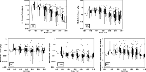
Regression analysis of the data (summarized in Table 3) showed that emission factors of all the pollutants exhibit statistically significant decreases over time, which suggests that older vehicles produce higher emissions (p ≤ 0.05 for all). The regression analysis also indicated that declines in BC and PM_2.5 with age (0.005< p <0.05) were not as strongly apparent compared to CO, NO_X, and UFP (p < 0.0001).

Table 3. Contribution of model year to emission factors.

	CO^a		NOX^a		BC^a		PM2.5^a		UFP^a
	β	p	β	p	β	p	β	p	β	p
Model year	–0.438	0.000	–0.302	0.000	–0.130	0.012	–0.148	0.005	–0.372	0.000

^aData were natural log-transformed to reduce variance and fulfill the distribution requirements of shown tests.

Vehicle technologies also have an equally important role on emission behavior. Since vehicle emission control programs in California have advanced tremendously over the last few decades, emission behavior was analyzed as a function of vehicle technology (Figure 4). The implementations of California’s low-emission vehicle (LEV) regulations were considered for vehicles based on their model year. The first LEV standards (LEV-I) applied to vehicle model years from 1994 through 2003, and the more stringent LEV-II regulations were applicable to model years 2004 through 2010 vehicles. Due to smaller sample sizes for vehicles with model years of pre-1994, no significant differences in emissions were observed. Therefore, all pre-1994 vehicles were classified as one group (pre-LEV).

Figure 4. Emission factors in different emission control technology groups.

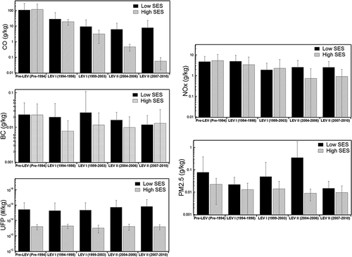
Analysis showed that CO emission factors reduced dramatically in vehicles after 1994 after the commencement of the first LEV program as compared to pre-LEV vehicles. Significant reductions were also observed in CO and NO_X emissions in LEV II (vehicles after 2004) from emissions from LEV I (vehicles between 1994 and 2003). We also found that older vehicles within the same technology group emitted more CO and NO_X emissions. All of the emission factors of vehicles with model years after 1994 show that emissions in low-SES regions were generally much higher compared to the high-SES area within the same category, with the CO emission factors showing a distinct stepwise reduction with each technological improvements in the high-SES community, whereas the emissions from low-SES vehicles show plateauing in LEV II technology vehicles. These differences were highlighted for UFP emissions, where the vehicle emissions from low-SES vehicles were an order of magnitude higher than their high-SES counterparts for each technology group. This suggests that emission behavior of vehicles in low-SES regions was influenced by other factors such as inadequate maintenance, higher mileage, or greater deterioration as compared to vehicles from the same technology groups in the high-SES community. It was also observed that vehicles in 2004–2006 had extremely high PM_2.5 emissions in low-SES areas as compared to their counterparts in the high-SES region. These findings suggest that vehicle age and technology do not explain the higher vehicular emissions in the low-SES communities. In the next section, we identify and characterize these super-emitters and estimate their contributions to the total emissions.

Super-emitters

The study also characterized real-world super-emitter vehicles in the sampled fleet by analyzing the distribution of vehicle emission factors of the sampled vehicles, and investigated the correlation of the prevalence of super-emitters with the socioeconomic status of the community. This analysis is intended to understand the real-world fat-tail emission distribution of light-duty passenger vehicles, and to study their characteristics and impacts on vehicular emissions and air quality in different socioeconomic regions in the state. This information may be useful to inform successful development and effective implementation of future emission mitigation programs and policies for mobile sources. For the purposes of this study, a super-emitter for each pollutant was defined as any vehicle that had an emission rate greater than 5 times the mean emission factors from all the vehicles in three cities. Table 4 indicates the cut points for identifying super-emitters in the measured light-duty gasoline vehicle fleet. In general, low-SES areas had higher occurrences of super-emitters. In total, 47 super-emitters were identified for all pollutants, which represents roughly 13% of the sampled fleet, and 13 vehicles were identified as super-emitters in more than two pollutants. The fraction of super-emitters found in this study was more than double the fraction found in Wilmington, CA, in 2007, which reported approximately 5% of the LDGVs as high-emitters using the same operational definition to identify super-emitters (5 times the fleet-average values). This observed increase in super-emitter fraction is very likely due to a significant increase in the number of low-emitting vehicles in the fleet, which is expected to lower the fleet average emissions, and subsequently lower the super-emitter thresholds (5 times the fleet average emission factor). As additional cleaner vehicles are introduced in the fleet, the average emission factors are expected to decrease, which will both distinguish the super emitter signature and cause an increase in their proportion to the motor vehicle fleet emissions. This would also highlight the importance of controlling super-emitters as a viable mitigation option to control their disproportionately higher contributions to the motor vehicle emissions.

Table 4. Identification of super-emitters in three cities.

		CO	NOX	BC	PM2.5	UFP
Total fleet-average EFs (g/kg)		32.7	3.1	0.02	0.05	^a3.7 × 10^14
Emission cut points to identify super-emitters;5 × total fleet-average EFs (g/kg)		163.6	15.6	0.09	0.27	^a1.9 × 10^15
Number of super-emitters	H	3	2	2	0	3
	L1	8	3	3	6	9
	L2	7	3	5	1	5
	Total	18	8	10	7	17

^aNumber/kg.

Low-SES areas had significantly greater occurrences of super-emitters (39 of the 47 super-emitters), whereas only 8 super-emitters were found in the high-SES area. When comparing the prevalence of super-emitters by SES, an average low-SES community (average of L1 and L2) had twice the number of super-emitters for CO, BC, and UFP than a high-SES community. The distribution disparity was especially pronounced for PM_2.5 super-emitters, where all of them were concentrated in low-SES communities.

Table 5 shows the comparisons of average model year and odometers of super-emitters compared to non-super-emitters. The average model year of all the super-emitters was 1992 with an average odometer reading of 142,214 miles. These data show that super-emitters were significantly older than the rest of the fleet; however, they had accrued similar or less mileage than their non-super-emitter counterparts. This suggests that deterioration due to vehicle use is a potentially less important contributor to emission behavior than original control technology (vehicle age). Even within the same technology group, super-emitters had lower average mileage, suggesting the importance of other confounding variables such as vehicle maintenance history or exceptional engine failure on vehicle emission behavior. Overall, CO and UFP super-emitters were likely to be much older than BC and PM_2.5 super-emitters, and UFP super-emitters had the highest average odometer among all. These findings disagree with findings from a study of on-road taxi data in Chicago, IL, that found that taxis that accumulate mileage faster than the regular fleet have a higher percentage of “high emitters” (Bishop and Stedman, 2008), suggesting a correlation between super-emitters and higher mileage.

Table 5. Identification of super-emitters in three cities.

		Sample size	Average model year	Average odometer (miles)
Super-emitters	CO	18	1986	136K
	NOX	8	1993	128K
	BC	10	1997	117K
	PM2.5	7	1996	138K
	UFP	17	1990	169K
Non-super-emitters		330	2000	143K

In order to review the emission certification history of the sampled vehicles, we evaluated vehicle records in the California Smog Check program database (California Smog Check Program, n.d.). California’s Smog Check Program is a vehicle emissions inspection program that is an important part of California’s efforts to improve regional and local air quality. Smog Check inspections are designed to identify and either repair or retire high-polluting vehicles, and classify vehicles as passing, failing, and gross polluting vehicles. Smog Check inspections are required biennially for all vehicles except gasoline powered vehicles 1975 and older, diesel-powered vehicles 1997 year model and older or with a gross vehicle weight rating (GVWR) of more than 14,000 lb, electric vehicles, natural-gas-powered vehicles over 14,000 lb, motorcycles, or trailers. Also, vehicles 6 or fewer model years old are also exempt from a biennial smog certification, and are instead required to pay an annual smog abatement fee for the first six registration years.

Multiple years of Smog Check records (2007 through 2010) were examined for the sampled vehicles to investigate whether super-emitters had recently failed smog check results. It should be noted that vehicles that were model year 1975 and older and vehicles less than 4 years old (2007–2010) were exempt from the program during the study period. The database showed that 254 vehicles out of total 378 LDGVs had Smog Check records, and 51 cars (20%) had multiple test results on the same day, suggesting that the vehicles were either gross polluters or failed during the initial test, and eventually passed with or without repair process. Only four cars had failed smog check records, and all of them were mid to late 1980s model year vehicles. This result agreed well with a previous study that found disproportionate numbers of failed vehicles of pre-1991 model year vehicles, and suggested that vehicles manufactured in 1980s with first-generation emissions technology are more likely to fail Smog Check (Choo et al., 2007).

Out of the 47 vehicles that were identified as super-emitters in this study, 12 vehicles did not have Smog Check records due to their model year (i.e., pre-1975, post-2006), DMV registration status, or disagreements between the vehicle type observed during the study and the registration information found in the DMV records. Furthermore, six vehicles had multiple Smog Check test records on the same day with at least one record of fail or gross polluter. Since every vehicle that fails the Smog Check test either gets retested or obtains necessary repairs to pass the test as a prerequisite for vehicle registration, this could indicate that vehicles resurfacing as super-emitters in real-world testing could be encountering failed repairs within the 2-year Smog Check certification period. The remaining 35 super-emitters had passed the Smog Check test within the last 2 years, representing a roughly 9% refail rate in real-world setting. This observation is consistent with a study conducted by Sierra Research, which found between 10-19% of the vehicles that had initially passed Smog Check had failed a roadside emissions test within one year (CARB/BAR, 2009). These findings suggest either that the real-world super-emitter emission behaviors are not being captured effectively in the Smog Check program, or that the Smog Check program needs to be further scrutinized (including increasing test frequency requirements) to improve its effectiveness. However, larger market penetration of self-diagnosing OBD systems and improvements to the Smog Check Program undertaken in the past few years are expected to improve program performance and to help in early diagnosis of emission control failure, as well as catching higher emitting vehicles during testing, which should help reduce the occurrence and impacts of super-emitters in the real world.

Vehicle contributions to fleet-average emission factors and co-pollutant emissions

The data obtained from individual vehicles were analyzed to evaluate their contribution to the fleet-average emission factors and the total fleet-wide emissions. These data are useful to understand emission contributions from higher emitting vehicles, and help understand the emission co-benefits of any potential control strategies. Since the number of super-emitters varied by pollutants, we analyzed the top 5-percentile emitters for each pollutant in each city for consistency. Figure 5 shows emission factor distribution of top 20% of the emitters in the three cities, and compares the prevalence of high emitters and the emission rates of top 20% fleet in each region. The steepness of slopes of the resultant graph indicates the significance of contributions of super-emitters to the fleet-wide emissions, and the figures indicated that the emission rates for the super emitters were generally an order of magnitude higher than the remaining fleet. It was observed that the high-SES community had a higher degree of skewness for CO and NO_X, whereas the low-SES communities had a higher degree of skewness for PM_2.5 and BC (L1 and L2, respectively). UFP distributions in three cities were very similar, although nominal values were lower in the high-SES community. Furthermore, the high-SES fleets had distinctly lower CO, NO_X, and PM_2.5 emission factors as compared to the sampled fleets in the low-SES communities. A few extreme super-emitters were found for CO, BC, and PM_2.5 in low-SES communities, while super-emitters of NO_X and UFP in three cities had emission factors in comparable ranges. On the other hand, there was very little evidence regarding the prevalence of super-emitters for PM_2.5 and BC in the high-SES community within the sampled fleet. These observations suggest that low-SES communities may be more impacted by particulate matter pollution from individual super-emitter vehicles.

Figure 5. Emission factors of individual vehicles in descending order.

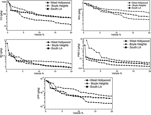
Table 6 presents the emission factors for the top 5th percentile of total LDGVs in each city. During the sampling period, the emission factors of the top 5th percentile of the vehicles in low-SES areas were an order of magnitude higher than for the entire sampled fleet for CO, BC, PM_2.5, and UFP. It was also noteworthy that the top 5th percentile PM_2.5 emitters in L1 emitted about 15 times more than the mean PM_2.5 emission factors of the sampled fleet. For the high-SES community, the emission factors of the top 5th percentile emitters were much lower as compared to those from the low-SES communities. For UFP, the top 5th percentile emitters in each of the three cities had similar contributions to their total UFP emissions (42–49%) during the study period. These observations are important in improving our understanding of the contributions of super-emitter vehicles to vehicular emissions. Since the actual annual operations of these vehicles is not available, and not all vehicles are operated equally, emission factors alone cannot directly elucidate the contributions of these vehicles to regional air quality. However, the prevalence of super-emitters in the low-SES areas during the testing period does indicate a relatively larger impact of these vehicles to local air quality in the region.

Table 6. Fleet-average emission factors for the top 5th percentile of the sampled LDGVs (total fleet-average emission factors in parentheses).

Location	CO (g/kg)	NOX (g/kg)	BC (g/kg)	PM2.5 (g/kg)	UFP (number/kg)
Boyle Heights (L1)	369 (37)	15.1 (3.8)	0.10 (0.02)	1.90 (0.11)	3.8 × 10^15 (5.0 × 10^14)
Southeast Los Angeles (L2)	417 (47)	16.4 (3.5)	0.21 (0.02)	0.48 (0.04)	4.0 × 10^15 (4.1 × 10^14)
West Hollywood (H)	199 (15)	14.4 (2.0)	0.07 (0.01)	0.06 (0.01)	2.5 × 10^15 (2.3 ×10^14)

These observations also highlight the importance of the comprehensive emission control program in California designed to help mitigate air pollution in the state, including car scrappage programs such as the California’s Enhanced Fleet Modernization Program, and other incentive programs such as Consumer Assistance Program (CAP) and Voluntary Accelerated Vehicle Retirement (VAVR) program that are intended to retire older and more polluting vehicles. These funding opportunities should help remove some super-emitters from the fleet, and decrease the occurrence and impact of high polluting vehicles in the future.

The emission co-benefits were calculated by analyzing the associations and correlations between the different pollutants using Spearman’s correlation coefficients between each set of pollutants (shown in Table 7). The results suggest that although the correlation coefficients (slopes) for the intercorrelations between different pollutants were small, their correlations were statistically significant in general (p < 0.01). It was also observed that emissions of CO were moderately correlated with NO_X. Furthermore, BC and PM_2.5 were moderately correlated with each other; while UFP emission was moderately correlated with emissions of all the pollutants. The observed overlap between certain pollutant super-emitters also suggests similarities in their emission behaviors, which may be useful in devising effective multipollutant mitigation strategies.

Table 7. Spearman correlation coefficients between different pollutant emission factors.

	CO	NOX	BC	PM2.5	UFP
CO	1.000	0.507	0.244	0.304	0.441
NOX		1.000	0.289	0.339	0.456
BC			1.000	0.427	0.451
PM2.5				1.000	0.412
UFP					1.000

Note. Correlation is significant at the 0.01 level (two-tailed), and the sample number (N) is 378.

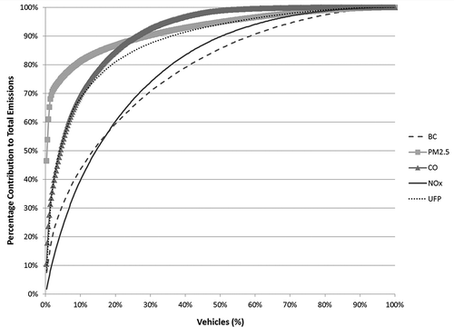
The observed emission factors were used to calculate annual vehicle emissions (tons/vehicle) in order to study the contributions of individual LDGVs to the total emissions. This analysis multiplied the emission factors (g/kg fuel) against the fuel consumption estimates (gallon/vehicle/year) extracted from EMFAC2011 by model year, vehicle type (passenger car vs. truck), and populations for Los Angeles County. The total emissions were obtained by integrating emissions of all 363 vehicles for which valid registration and vehicle make and model year information were available (15 vehicles were excluded in the calculation due to lack of registration information). It should be noted that this calculation uses vehicle use statistics extracted from EMFAC, and assumes that newer vehicles are driven more than older vehicles and that all vehicles of a particular model year are driven equally (irrespective of their region’s SES conditions or vehicle emitter status). Cumulative emission distributions of sampled vehicles are shown in Figure 6. For the sampled fleet, approximately 15% of the vehicles contributed half of the total emissions for BC and NO_X, whereas less than 5% of the vehicles contributed about half of the total emissions for PM_2.5, CO, and UFP. Since these highest percentile ranks are dominated by super-emitters, these results highlight the importance of controlling super-emitters (by either repairing, retrofitting, replacing, or retiring these vehicles) as a low-hanging fruit for reducing vehicular emissions. Table 8 also shows the contributions of the top 5th percentile vehicles for each pollutant to the total emissions of all other pollutants, and highlights the co-benefits of controlling the higher emitters for one pollutant would also have significant co-pollutant emission reduction benefits. In general, it is observed that controlling the top 5th percentile vehicles for PM_2.5 would yield the highest co-benefits, with more than 75% reduction in PM_2.5 emissions, and roughly 10–20% reduction for all other pollutants. Such efforts will offer immediate returns in air quality improvements, and will reduce air quality and health impacts for drivers and passengers, as well as in microenvironments in the immediate vicinity of the vehicles including traffic signals, congested freeways, and parking lots.

Table 8. Contribution of the top 5th percentile emitters to the total emissions.

Responsiblefor	BC (%)	PM2.5 (%)	CO (%)	NOX (%)	UFP (%)
Top 5% BC	31.3	12.6	9.8	8.6	13.0
Top 5% PM2.5	11.9	75.8	17.5	8.6	22.0
Top 5% CO	6.0	3.5	53.0	7.0	6.3
Top 5% NOX	10.5	2.3	3.5	23.8	2.8
Top 5% UFP	10.6	11.1	7.4	6.9	53.6

Figure 6. Cumulative contributions of individual vehicles to the total emissions.

Conclusions

This study focused on real-world emission behavior and super-emitter distribution of light-duty gasoline vehicles in different regions, and investigated the relationship of on-road vehicle emissions with local socioeconomic conditions of the region. It was hypothesized that as the overall fleet emissions have decreased due to more stringent regulations, a small fraction of the fleet may be contributing a disproportionate share of the overall on-road vehicle emissions.

The study observed a significant reduction in vehicle emissions for all measured pollutants when compared to a similar regional study in Wilmington, CA, in 2007, with as much as 30–60% reductions in sampled fleet emissions as compared to the earlier sampled fleet. Although the real scales of reductions in emission factors are expected to be less than the observed reductions due to methodological improvements, the measurement data from this study strongly indicates that vehicle emission have decreased in the low-SES areas as compared to the earlier study. The study also found a positive correlation between the socioeconomic status of a community and the prevalence of high-emitting vehicles. Vehicles in low-SES communities were approximately 4–5 years older than vehicles in a high-SES community, and their emission factors were 2–3 times greater for CO, NO_X, BC, and UFP and 4–11 times greater for PM_2.5 when compared to the high-SES neighborhood.

Vehicle emissions calculated using observed emission factors and model year-specific activity data from EMFAC indicated that approximately 5% of the sampled vehicles in each city accounted for nearly half of the total CO, PM_2.5, and UFP emissions from the sampled fleet, and 15% of the vehicles were responsible for more than half of the total NO_X and BC emissions. Results showed that super-emitters are present in older as well as newer model year vehicles for BC and PM_2.5, indicating that the super-emitters identified by this study are not merely older vehicles that were certified to higher emission standards, but are true super-emitters in the real-world settings. It was also observed that vehicles in low-SES areas had higher PM_2.5 emissions for the same model year, suggesting that vehicle age and technology do not alone explain the higher vehicular emissions in the low-SES communities, and other factors (such as mileage and maintenance history) may have a significant impact on vehicle’s emission behavior. It also signifies the importance of proper maintenance and compliance with the Smog Check programs, and highlights their significance in improving air quality at the community-level.

Since the current study was based on a limited data set of vehicles, investigation of a larger data set would be beneficial to obtain a more comprehensive reflection on region-wide on-road vehicle emission distributions. The study was unable to measure total hydrocarbons (THC) due to unavailability of appropriate instrumentation during the measurement campaign. Hydrocarbons are known to have very highly skewed emission distributions for super-emitters and will benefit from additional studies. As the fleet characteristics change over time, routine studies may be also useful to better classify and understand the effect of super-emitters on regional emissions and community air quality, and for developing effective emission control and mitigation strategies.

Disclaimer

The statements and opinions expressed in this paper are solely the authors’ and do not represent the official position of the California Air Resources Board. The mention of trade names, products, and organizations does not constitute endorsement or recommendation for use.

Acknowledgment

The authors would thank Toyota for its support in providing a Toyota RAV4 EV for this research. They also thank CARB staff who assisted in data collection and interpretation and in providing valuable comments during the review process, with special thanks to Walter Ham, Toshihiro Kuwayama, Chris Ruehl, Sam Pournazeri, Sherrie Sala-Moore, and Kathy Jaw.

Additional information

Notes on contributors

Seong Suk Park

Seong Suk Park, Abhilash Vijayan, Steve L. Mara, and Jorn D. Herner conducted this research for the Research Division of the California Air Resources Board, located in Sacramento, CA.

Abhilash Vijayan

Seong Suk Park, Abhilash Vijayan, Steve L. Mara, and Jorn D. Herner conducted this research for the Research Division of the California Air Resources Board, located in Sacramento, CA.

Steve L. Mara

Seong Suk Park, Abhilash Vijayan, Steve L. Mara, and Jorn D. Herner conducted this research for the Research Division of the California Air Resources Board, located in Sacramento, CA.

Jorn D. Herner

Seong Suk Park, Abhilash Vijayan, Steve L. Mara, and Jorn D. Herner conducted this research for the Research Division of the California Air Resources Board, located in Sacramento, CA.

References

- Ban-Weiss, G.A., J.P. McLaughlin, R.A. Harley, M.M. Lunden, T.W. Kirchstetter, A.J. Kean, A.W. Strawa, E.D. Stevenson, and G.R. Kendall. 2008. Long-term changes in emissions of nitrogen oxides and particulate matter from on-road gasoline and diesel vehicles. Atmos. Environ. 42(2):220–32. doi:10.1016/j.atmosenv.2007.09.049
- Bishop, G.A., and D.H. Stedman. 2008. A decade of on-road emissions measurements. Environ. Sci. Technol. 42:1651. doi:10.1021/es702413b
- Cadle, S.H., P. Mulawa, E.C. Hunsanger, K. Nelson, R.A. Ragazzi, R. Barrett, G.L. Gallagher, D.R. Lawson, K.T. Knapp, and R. Snow. 1999. Light-duty motor vehicle exhaust particulate matter measurement in the Denver, Colorado, area. J. Air Waste Manage. Assoc. 49:164. doi:10.1080/10473289.1999.10463872
- California Air Resources Board. 2013. California Almanac of Emissions and Air Quality—2013 Edition. http://www.arb.ca.gov/aqd/almanac/almanac13/almanac13.htm
- California Air Resources Board. 2011. Emission Factor Model (EMFAC) 2011. http://www.arb.ca.gov/msei/modeling.htm ( accessed 2013).
- California Air Resources Board. 2007a. Emission Factor Model (EMFAC) Modeling Change Technical Memo on Modification of Mileage Accrual Rates. http://www.arb.ca.gov/msei/onroad/techmemo/modified_mileage_accrual_rates.pdf ( accessed 2015).
- California Air Resources Board. 2007b. Research Contract No. 05-323; Light Duty Gasoline PM: Characterization of High Emitters and Valuation of Repairs for Emission Reduction, October. Prepared by T.D. Durbin, J.F. Collins, and W. Li, College of Engineering-Center for Environmental Research and Technology, University of California Riverside, Riverside, CA.
- California Air Resources Board and California Bureau of Automotive Repair. 2009. Evaluation of the California Smog Check Program Using Random Roadside Data; Report No. SR09-03-01, Prepared by Sierra Research, Inc., March.
- California Smog Check Program. n.d. http://www.bar.ca.gov/FormsPubs/Q&As_Smog_Check_Program.html ( accessed 2015).
- Choi, W., S. Hu, M. He, K. Kozawa, S. Mara, A.M. Winer, and S.E. Paulson. 2013. Neighborhood-scale air quality impacts of emissions from motor vehicles and aircraft. Atmos. Environ. 80:310–21. doi:10.1016/j.atmosenv.2013.07.043
- Choo, S., K. Shafizadeh, and D. Niemeier. 2007. The development of a prescreening model to identify failed and gross polluting vehicles. Transport. Res. Part D Transp. Environ. 12(3):208–18. doi: 10.1016/j.trd.2007.01.012
- City Data Website. n.d. http://www.city-data.com ( accessed 2013).
- Collet, S., T. Kidokoro, Y. Kinugasa, P. Karamchandani, and A. DenBleyker, A. 2015. High emitter light duty vehicle contributions to on-road mobile emissions in 2018 and 2030. Stud. Eng. Technol. 2(1):47–53. doi:10.11114/set.v2i1.838
- Garshick, E., F. Laden, J.E. Hart, and A. Caron. 2003. Residence near a major road and respiratory symptoms in U.S. veterans. Epidemiology 14(6):728–36. doi:10.1097/01.ede.0000082045.50073.66.
- Geller, M.D., S.B. Sardar, H. Phuleria, P.M. Fine, and C. Sioutas. 2005. Measurements of particle number and mass concentrations and size distributions in a tunnel environment. Environ. Sci. Technol. 39(22):8653–63. doi:10.1021/es050360s
- Kirchstetter, T.W., R.A. Harley, N.M. Kreisberg, M.R. Stolzenburg, and S.V. Hering. 1999. On-road measurement of fine particle and nitrogen oxide emissions from light-and heavy-duty motor vehicles. Atmos. Environ. 33(18):2955–68.
- Kozawa, K.H., S.S. Park, S.L. Mara, and J.D. Herner. 2014. Verifying emission reductions from heavy-duty diesel trucks operating on Southern California freeways. Environ. Sci. Technol. 48(3):1475–83. doi:10.1021/es4044177
- Lawson, D.R., P.J. Groblicki, D.H. Stedman, G.A. Bishop, and P.L. Guenther. 1990. Emissions from in-use motor vehicles in Los Angeles: A pilot study of remote sensing and the inspection and maintenance program. J. Air Waste Manage. Assoc. 8:1096–1105. doi:10.1080/10473289.1990.10466754
- O’Neill, M.S., M. Jerrett, I. Kawachi, J.I. Levy, A.J. Cohen, N. Gouveia, P. Wilkinson, T. Fletcher, L. Cifuentes, and J. Schwartz. 2003. Health, wealth, and air pollution: advancing theory and methods. Environ. Health Perspect. 111(16):1861–70. doi:10.1289/ehp.6334
- Park, S.S., K. Kozawa, S. Fruin, S. Mara, Y.K. Hsu, C. Jakober, A. Winer, and J. Herner. 2011. Emission factors for high-emitting vehicles based on on-road measurements of individual vehicle exhaust with a mobile measurement platform. J. Air Waste Manage. Assoc. 61(10):1046–56. doi:10.1080/10473289.2011.595981
- Ramanathan, V., and G. Carmichael. 2008. Global and regional climate changes due to black carbon. Nat. Geosci. 1:221. doi:10.1038/ngeo156
- Shah, S.D., K.C. Johnson, J. Wayne Miller, and D.R. Cocker III. 2006. Emission rates of regulated pollutants from on-road heavy-duty diesel vehicles. Atmos. Environ. 40(1): 147–53. doi:10.1016/j.atmosenv.2005.09.033
- Shorter, J.H., S. Herndon, M.S. Zahniser, D.D. Nelson, J. Wormhoudt, K.L. Demerjian, and C.E. Kolb. 2005. Real-time measurements of nitrogen oxide emissions from in-use New York City transit buses using a chase vehicle. Environ. Sci. Technol. 39(20):7991–8000. doi:10.1021/es048295u
- Singer, B.C., and R.A. Harley. 2000. A fuel-based inventory of motor vehicle exhaust emissions in the Los Angeles area during summer 1997. Atmos. Environ. 34(11):1783–95. doi:10.1016/S1352-2310(99)00358-1
- Tan, Y., E.M. Lipsky, S. Saleh, A.L. Robinson, and A.A. Presto. 2014. Characterizing the spatial variation of air pollutants and the contributions of high emitting vehicles in Pittsburgh, PA. Environ. Sci. Technol. 48(24):14186–94. doi:10.1021/es5034074.
- Zhang, Y., D.H. Stedman, G.A. Bishop, P.L. Guenther, and S.P. Beaton. 1995. Worldwide on-road vehicle exhaust emissions study by remote sensing. Environ. Sci. Technol. 29(9): 2286–94. doi:10.1021/es00009a020