Human-model hybrid Korean air quality forecasting system

ABSTRACT

The Korean national air quality forecasting system, consisting of the Weather Research and Forecasting, the Sparse Matrix Operator Kernel Emissions, and the Community Modeling and Analysis (CMAQ), commenced from August 31, 2013 with target pollutants of particulate matters (PM) and ozone. Factors contributing to PM forecasting accuracy include CMAQ inputs of meteorological field and emissions, forecasters’ capacity, and inherent CMAQ limit. Four numerical experiments were conducted including two global meteorological inputs from the Global Forecast System (GFS) and the Unified Model (UM), two emissions from the Model Intercomparison Study Asia (MICS-Asia) and the Intercontinental Chemical Transport Experiment (INTEX-B) for the Northeast Asia with Clear Air Policy Support System (CAPSS) for South Korea, and data assimilation of the Monitoring Atmospheric Composition and Climate (MACC). Significant PM underpredictions by using both emissions were found for PM mass and major components (sulfate and organic carbon). CMAQ predicts PM_2.5 much better than PM₁₀ (NMB of PM_2.5: -20~-25%, PM₁₀: -43~-47%). Forecasters’ error usually occurred at the next day of high PM event. Once CMAQ fails to predict high PM event the day before, forecasters are likely to dismiss the model predictions on the next day which turns out to be true. The best combination of CMAQ inputs is the set of UM global meteorological field, MICS-Asia and CAPSS 2010 emissions with the NMB of -12.3%, the RMSE of 16.6μ/m³ and the R² of 0.68. By using MACC data as an initial and boundary condition, the performance skill of CMAQ would be improved, especially in the case of undefined coarse emission. A variety of methods such as ensemble and data assimilation are considered to improve further the accuracy of air quality forecasting, especially for high PM events to be comparable to for all cases.

Implications: The growing utilization of the air quality forecast induced the public strongly to demand that the accuracy of the national forecasting be improved. In this study, we investigated the problems in the current forecasting as well as various alternatives to solve the problems. Such efforts to improve the accuracy of the forecast are expected to contribute to the protection of public health by increasing the availability of the forecast system.

Introduction

Regional air pollution can have adverse effects on global air quality through hemispheric and intercontinental transport (HTAP, 2010). If the more local source is reduced by emission control, the more local air quality is prone to the long-range transport of air pollution. Northeast Asia has experienced rapid economic growth since the 1970s accompanied by the rapid increase of the emission of air pollutants. The air pollutants emissions from Northeast Asia might exceed those from the United States and Europe from the late 1990 (Stohl and Eckhardt, 2004). For example, the anthropogenic NOx emission in Asian regions in the late 1990s approached 30,000 kton annually, and it started to exceed that in the United States and Europe (Akimoto, 2003). Moreover, the emission in the United States and Europe shows a trend of decrease, whereas the emission in Northeast Asia shows a trend of rapid increase (Amann et al., 2013). Unless special measures are taken, this trend of emission increase will continue, posing a threat to Northeast Asia as well as to the global atmospheric environment. Air pollutants are known to aggravate visibility and cause respiratory, cardiovascular, and immunological diseases (World Health Organization, 2004; Davidson et al., 2005; Phalen and Phalen, 2011). They cause smog all throughout the region and have bad effects on regional weather phenomena (Seinfeld and Pandis, 2006).

As the Asian emissions exceed a certain threshold level, severe air pollution tends to occur easier. Recently, the frequent smog in China has raised the awareness of Koreans on particulate matters (PM). It is known that PM_2.5, which is about 1/30 times as thick as a strand of hair, poses a very high risk to the human body because it flows in the blood and spreads to the whole body, causing various diseases, such as respiratory diseases and cerebral infarction, and enhancing mortality (e.g. Thurston et al., 1994; Schwartz et al., 1996; Pope, 2000). In 2013 and 2014, the whole area of China was inflicted with extreme smog, signaling a warning light to the air quality of its neighboring countries. Eventually, the smog also frequently occurred in Korea, and people started to ask the government to strongly cope with it to protect their health. Under these circumstances, the Ministry of Environment and the National Institute of Environmental Research commenced a PM forecast system on a pilot basis on August 31, 2013, targeting Seoul metropolitan area (SMA); expanded the forecast region to the whole country on December 31, 2013; and enforced the forecast system in earnest from February 06, 2014. Later, the forecast substance was expanded to ultrafine particulate and ozone (May 30, 2014).

The growing utilization of the forecast induced the public strongly to demand that the accuracy of the national forecasting be improved. Accordingly, we investigated the problems in the current forecasting as well as various alternatives to solve the problems. Such efforts to improve the accuracy of the forecast are expected to contribute to the protection of public health by increasing the availability of the forecast system.

The national air quality forecasting

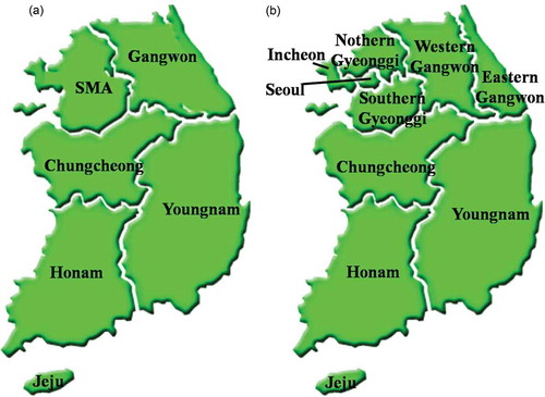
The forecasting systems of several countries were compared in the aspects of forecast organization, commencement and target pollutants as in Table 1. The United States, the United Kingdom, France, and Germany already started the forecast system from the 1990s or the early 2000s, and they generally issue comprehensive air quality index (AQI) on website by combining 2–6 kinds of major air pollutants. Instead of comprehensive AQI, Korea used air quality level (AQL) for individual air pollutants in terms of health risk. For example, five categories, such as Good(0–30µg/m³), Normal(31–80µg/m³), Slightly Bad(81–120µg/m³), Bad(121–200µg/m³), and Very Bad(>200µg/m³), based on 24-h averaged PM₁₀ concentration, is used as AQL for PM that is an interesting pollutant in this study. Forecasting period can be divided into two stages; initial stage (31, Aug., 2013 ~ 4, Feb., 2014) and regular stage (5. Feb. 2015~). During the initial stage, spatially, as shown in Figure 1a, the regional averaged AQL is used by dividing the whole country into six areas (the Seoul metropolitan area, the Gangwon area, the Chungcheong area, the Honam area, the Yeongnam area, and the Jeju area). During the regular stage, this regional division in the SMA and Gangwon regions were subdivided into the four and two regions as following: SMA is into Seoul, Incheon, the northern and southern Gyeonggi region, and Gangwon is into the Yeongseo and the Yeongdong region (Figure 1b). In addition, the five categories were reduced to four categories by combining the levels of Slightly Bad and Bad in order to avoid the public’s confusion and the Very Bad level over 200 µg/m³ was lowered to 150 µg/m³.

Table 1. Comparison of world-wide national air quality forecasting systems by executing organization, start year, and target pollutants.

Country	Executing organization	Start year	Target pollutants
United States	EPA (http://airnow.gov/), National Oceanic Atmospheric Administration	‘99~	Air Quality Index (AQI) for O3 and PM2.5 divided into six categories (good, moderate, unhealthy for sensitive groups, unhealthy, very unhealthy, hazardous).
Germany	Rhenish Institute for Environmental Research (http://www.uni-koeln.de/math-nat-fak/geomet/eurad)	‘04~	AQI for five pollutants (O3, NO2, PM10, SO2, CO) divided into six categories (very good, good, satisfactory, sufficient, poor, very poor).
France	INERIS, METEO-France (http://www.prevair.org)	‘03~	Three pollutants (O3, NO2, PM,) with maps representing average concentration and maximum daily.
United Kingdom	DEFRA (http://uk-air.defra.gov.uk/forecasting/)	‘90~	Daily AQI for five pollutants (O3, NO2, SO2, PM10, PM2.5) using a combination of numbers (1–10) and words (very good, good, satisfactory, sufficient, poor, very poor) and colors (green/yellow/orange/red/purple).

Figure 1. Forecasting area at (a) the initial stage, (b) present.

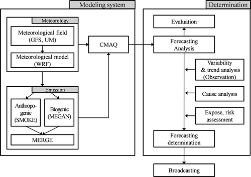
The forecast cycle was expanded from two times/day in the initial stage of the enforcement to four times per day upon public request, and the forecast time is synchronized with the weather forecast time and fixed at 05:00 a.m., 11:00 a.m., 05:00 p.m., and 11:00 p.m. in local time daily. The forecast is finally issued as the decision-making by the forecaster based on the model results with his knowledge, experience, and knowhow. The process of air quality forecasting system is shown in Figure 2. The process, for example, on the forecasting time of 5pm, is listed on timeline as follows: (1) the meteorological data is downloaded at 9 a.m. and (2) the predicted results from model are produced at 2 p.m. After that, as act of determination, (3) a forecaster analyses an air quality pattern with predicted and observed data and (4) it is discussed at 4 p.m., finally (5) at 5 p.m., AQL is decided. In present, the human factor was promoted as the central part of the national forecasting as the operational forecaster gains experience.

Figure 2. Schematic diagram of the national air quality forecast system.

The performance of the national forecasting is regularly analyzed using near real-time measurement data. In regular assessment, traditional and categorical statistics including accuracy and critical success index (CSI) were used as shown in Table 2.

Table 2. Statistics measures used in the forecast and model evaluation (complied from Boylan and Russell, 2006; Zhang et al., 2012a).

Target	Measure	Mathematical Expression	Range
Forecast*	Accuracy		0% to 100%
	Critical Success Index (CSI)		0% to 100%
	False Alarm Rate (FAR)		0% to 100%
Model value**	Mean Fractional Bias (MFB)		−200% to +200%
	Mean Fractional Error (MFE)		0% to +200%
	Normalized Mean Bias (NMB)		−100% to +∞
	Root Mean Square Error (RMSE)		O to +∞

Notes: * N is the number of samples (by time and/or location). Where a, b, c, d represent simulated AQL while 1,2,3,4,5 represent observed AQL (a & 1: ‘good’, b & 2: ‘normal’, c & 3: ‘slightly bad’, d & 4: ‘bad’, e & 5: ‘very bad’). I, II, III, IV represent forecast nonexceedances that did occur, forecast exceedances that did not occur, forecast nonexceedances that did not occur, and forecast exceedance that did occur, respectively

** M and O are 24h averaged simulated and observed values in SMA .

Looking at the temporal change in the forecast accuracy after the enforcement of the forecast system, the accuracy of model+human factor decreased to lower than 60% in the initial stage of the forecast. But after increasing forecaster’s experience for about 2 years and adopting several modeling systems (refer to next section) such as experiment 1 and 2 and changing forecasting system, dividing forecast regions detailedly and reducing categories, it recovered to 80~90% in regular stage. However, the hit rate of model itself without human factor is still lower to 48~69% depending on model inputs, such as meteorological fields and emissions. CSI of model and human factor increased by just 10~20%, from 30~40% in the initial stage to 50~60%, while CSI of model itself ranges 17~41%. It is known that exposure to the high PM event increases the number of respiratory outpatients or aggravates their respiratory symptoms, causing a significant damage to their health. Accordingly, we investigated the cause of false forecasting and the method of its improvement, targeting PM pollution episodes with great health damage.

National Air Quality Forecasting Modeling System

National Air Quality Forecasting Modeling System (NAQFMS) largely consists of a meteorological model, the Weather Research and Forecasting (WRF) v3.3 (Michalakes et al., 2001), and emission process models, the Sparse Matrix Operator Kernel Emissions (SMOKE) v3.1 (Houyoux and Vukovich, 1999) and the Model of Emissions of Gases and Aerosols from Nature (MEGAN) v2.04 (Guenther et al., 2006), and a chemical transport model, the Community Modeling and Analysis (CMAQ) v4.7.1 (Byun and Ching, 1999) (Figure 2).

In the initial stage of NAQFMS, the Global Forecast System (GFS) data of National Centers for Environmental Prediction (NCEP) was used as the input of WRF, but after June 08, 2014, the forecast data of Met Office Unified Model (UM), which is operational weather forecasting model of Korea Meteorological Administration, was added. The Model Intercomparison Study Asia of 2010 (MICS-Asia) (Carmichael et al., 2002), International Chemical Transport Experiment-Phase B(INTEX-B) (Zhang et al., 2009) and the Clear Air Policy Support System (CAPSS) inventory of 2007 from the National Institute of Environmental Research (NIER), were used for Asian and Korean emissions, respectively. Later, the base year of CAPSS was updated to 2010. These emission inventories are processed through spatial/temporal allocation and chemical speciation of SMOKE Modeling System. For new Source Classification Code (SCC) that is not in SMOKE SCC, the spatial/temporal allocation and chemical speciation were conducted by matching it with a similar SCC in SMOKE. Nine emission pollutants are considered: SO₂, NOx, CO, NMVOC, NH₃, PM₁₀, PM_2.5, BC, and OC. Emission sectors used in INTEX-B were so simplified that they were classified in more detail according to EDGAR 3.2 FT 2000: power generation, industry, residential, transportation, domestic animal & fertilizer use, wild animals, biofuel combustion, crop, human perspiration and respiration. Basically, SMOKE package such as monthly, weekly and diurnal profiles was adopted for temporal allocation. However, in order to correctly represent Asian activities, they were further modified with the help of a selective range of literature for Asian emissions temporal variation (Woo et al., 2012).

To save computational time, a pre-built database of weekly and monthly emissions from area and mobile sources are used while the emissions from point sources are daily updated according to meteorological forecast.

To estimate the biogenic emissions, MEGAN package for parameters (http://acd.ucar.edu/~guenther/MEGAN/MEGAN.htm) rather than localized ones was used. The reason is that, though Plant Functional Type (PTF) and Leaf Area Index (LAI) can be obtained from a satellite (e.g., Moderate-resolution Imaging Spectroradiometer, or MODIS), the other parameters such as emission factor, solar radiation/temperature correction factor are not available in Asian region. Hourly emission is estimated using MEGAN vegetation and emission data with 120-second resolution and the final emission is estimated by reclassifying it according to chemical mechanism and adding it up with anthropogenic emission. The sum of anthropogenic and biogenic emissions is used as Air-Quality Model (AQM) input together with the meteorological model result.

The regional air quality model used in NAQFMS is CMAQ, a certified model of EPA, which simulates the horizontal and vertical transport of the air pollutants as well as dry·wet deposition, and gas-phase and aerosol chemistry, etc. The post-processing models such as Brute-Force Method estimation, primary carbon apportionment, and sulfate tracking are used to quantify the contribution of domestic and foreign sources.

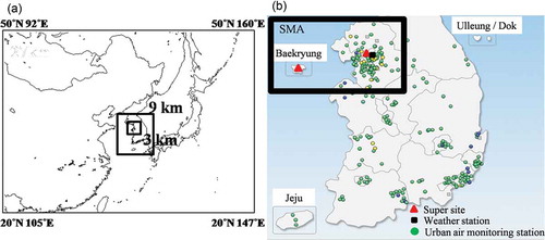
Three domains in CMAQ modeling cover Northeast Asia, the Korean peninsula, and the Seoul metropolitan area, with three different grid resolutions of 27, 9, and 3 km, respectively (Figure 3a). The Korean peninsula was set up to prevent the reduction of the predict ability of the Jeju region due to an error of the regional model boundary by including the southern part of Jeju Island. The SMA domain was also set up as slightly wider than the Gyeonggi province, considering the boundary error of the Korean peninsula domain. The central point of the modeling domain covered Northeast Asia is 37.5°N and 127°E, and the Lambert conformal conic map-projection parameters for both the mother and daughter domains were designed to be the same. Nesting method is adopted that finer resolution model (daughter) is embedded simultaneously within a coarser resolution model (mother) forecast. The last simulated model output was used as an initial condition for each modeling domain. The typical profiles provided by CMAQ model were used as lateral boundary condition of mother domain. The daughter models use the nested lateral boundary condition from mother model.

Figure 3. AQM modeling domains for NAQFMS. (a) Three model domains that have resolutions of 27km, 9km, 3km, respectively. (b) Spatial distribution of observations in South Korea; the Box is study area.

Method

To investigate the causes of the false forecasting of PM, several numerical experiments from NAQFMS are conducted as Table 3: control run (GFS and MICS-Asia/CAPSS2010), experiment 1 (UM, MICS-Asia/CAPSS2010), experiment 2 (GFS, INTEX-B/CAPSS2007), and experiment 3 (data assimilation). In particular, for data assimilation, the method of using the Monitoring Atmospheric Composition and Climate (MACC) (Inness et al., 2013) global forecast output was adopted. Based on several combinations of above experiments, the sensitivities of meteorology, emission AQM limit, and data assimilation to PM forecast were tested.

Table 3. Summarization of modeling experiments’ information.

	Control run	Experiment1	Experiment2
	GFS	UM	GFS	Experiment3
Meteorological model	WRFv3.3 Short wave radiation: Goddard (Chou and Suarez, 1999) Long wave radiation: RRTM (Mlawer et al., 1997) Land surface model: NOAH (Chen and Duhia, 2001) Planetary boundary layer: YSU (Hong et al., 2006) Cumulus convection: Kain-Fritsch (Kain, 2004) Cloud microphysics: WSM3 (Hong et al., 1998; Hong et al., 2004)			MACC Reanalysis (Inness et al., 2013)
Foreign Inventory	MICS-Asia 2010	MICS-Asia 2010	INTEX-B
National Inventory	CAPSS (base year:2010)	CAPSS (base year:2010)	CAPSS (base year:2007)
Emission model	SMOKEv3.1 (anthropogenic) MEGANv2.04 (biogenic)
Chemical transport model	CMAQv4.7.1 Aerosol module: Aero5 Advection: Priecewise Parabolic Method Vertical diffusion: Eddy viscosity (K-theory)
Time step	1hr	1hr	1hr	3hr
Domain resolution	27km, 9km, 3km			80km

To evaluate these experiments, model output from three experiments (control run, Exp.1, and Exp.2) available were compared to surface observation. Almost 2 year evaluation was performed from the start date of narional forecasting (30, Aug. 2013) to recent (30 June, 2015). Since AQMs with different input data have been adopted one by one since the inception of NAQFMS (UM Mar. 2014; INTEX-B Jan. 2014; MACC Nov. 2013), the model output availability is limited to date, 95.6% for the control run, 64.2% for Exp.1, 84.8% for Exp.2, and 79.5% for Exp.3 for the evaluation periods. At least 64.2% of the evaluation period was overlapped among the four experiments. Datasets for forecast evaluation include real-time or near real-time measurement datasets from the regular weather station data, urban air monitoring network data, and PM composition data of super sites operated by the National Institute of Environmental Research. The number of observatories used is 1 regular weather station in Seoul, 113 urban air monitoring stations in SMA, and Seoul and Baekryung island super sites (Figure 3b). The time resolutions are all 1 hr. In addition, the evaluation of PM prediction in experiments were conducted in terms of traditional performance statistics as shown in Table 2 such as Normalized Mean Bias (NMB), Root Mean Square Error (RMSE), and correlation coefficient (R²).

Result

Accuracy of air quality forecasting in modeling system

For PM, in the comparison of impacts of different meteorological fields, the PM forecast in control run (GFS, MICS-Asia /CAPSS2010) was overall poorer than that in Exp. 1 (UM, MICS-Asia /CAPSS2010) . The Normalized Mean Bias (NMB) and Root Mean Square Error (RMSE), and R² of the control run are -25.9%, 23.9µg/m³, and 0.59, respectively, whereas those of Exp. 1 are -12.2%, 16.6 µg/m³, and 0.67, respectively. However, in the comparison of impacts of different emissions, the forecasting skill of control run (GFS, MICS-Asia and/CAPSS2010) are used, was slightly better than that of Exp.2 (GFS, INTEX-B/and CAPSS2007). NMB, RMSE, and R² of Exp.2 showed -38.4%, 26.8 µg/m³, and 0.64, respectively. Therefore, Exp. 1 (UM, MICS-Asia/CAPSS2010) of AQM is most accurate than others.

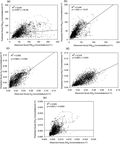
In addition, the comparison of the predicted daily mean NO₂, and SO₂, the precursors of PM, and O₃ in the control run is conducted with the surface observation in SMA. As shown in Figure 4c-e, R² of daily mean O₃, NO₂, and SO₂ concentration are 0.585, 0.576, and 0.000. This result illustrates that the uncertainty of AQM is high for not only PM (Figure 4a-b) but also other species.

Figure 4. Comparison of pollutants concentration between observation and model prediction for daily (a) PM₁₀, (b) PM_2.5, (c) O₃, (d) NO₂, (e) SO_2.

Cause of false forecasting and the improvement method

The accuracy of the national forecasting depends on the performance skill of both models and forecasters. Once an emission enters into AQM, AQM converts the emission to a concentration under various meteorological conditions. So an error occurs because of the inaccuracy of the emissions and the meteorological field, and inherent AQM limit (e.g. Seaman and Michelson, 2000; Baklanov et al., 2002; Zhang et al., 2012b). Furthermore, since forecasters make a final decision on AQL for PM next day, the lack of experience and knowledge of the forecasters is also one of causes of the error.

The false forecasting high PM events (‘bad’ and ‘very bad’ level) during the evaluation period except for Asian dust days were selected for cause analysis. During the period false forecasting high PM events numbered totally 55; 21 by over-forecasts and 34 by under-forecasts. For cause analysis, three experiments (Control run, Exp.1, and Exp.2) were established and all the false forecasting high PM events classified to the four factors (forecaster, meteorology, emissions, AQM); (1) forecaster factor when forecasters give the false forecast though the model matches well with the observation, (2) the meteorology factor when the control run and Exp.1 predict different AQLs or the difference for simulated PM₁₀ concentration is more than 20 µg/m³ corresponding to two sigma of difference distribution of PM₁₀ concentration for the evaluation period; (3) the emission factor when normalized error of the simulated PM₁₀ concentrations from either two emission models is more than 50%; (4) AQM factor when meteorological and emission factors are unexplainable and thus, it may be attributed to model uncertainties such as the initial / boundary conditions and chemical and physical parameterizations and so on. In other words, when a model result was correct but forecasting was failed, it is ‘forecaster’ factor. If both the model and forecasters were incorrect, the factors were examined in the order of NAQMS processing (meteorology→emission→AQM). As the result of analyzing the four causes of false forecasting on high PM events above mentioned, emission factor accounted for 29%; meteorology factor for 25%; forecaster factor for 36%; and AQM limit factor for 9% (Table 4). Strictly speaking, it is likely that multiple sources of uncertainty can cause the false forecasting together, but in this study, only dominant factor is considered. In addition, because criteria were not set upon absolute error of each factor, there is a limitation in interpreting each factor minutely. The overall model error including the meteorology, emission and AQM limit factors was attributed to almost 2/3 of false forecasting. The detailed analsys for each cause is illustrated in Table 4.

Table 4. List of false forecast dates classified by four factors including emission, meteorology, model, and forecaster with false alarm dates during 1 September 2013 ~ 31 June 2015.

Factors (number of days)	Date
Emission (16)	’13.12.5, ’13.12.30, ’14.1.22, ’14.1.30, ’14.2.17, ’14.2.25, ’14.3.4, ’14.3.15, ’14.4.16, ’14.4.23, ’14.5.2, ’14.5.13, ’14.5.14, ’14.7.15, ’14.7.27, ’15.2.5
Meteorology (14)	’13.11.2, ’13.11.24, ’13.12.20, ’14.1.17, ’14.1.21, ’14.2.28, ’14.3.1, ’14.3.16, ’14.6.2, ’14.6.17, ’15.1.16, ’15.3.3, ’15.3.8, ’15.3.18
Model limit (5)	’13.10.29, ’13.11.16, ’14.2.23, ’14.4.12, ’15.1.24
Forecaster (20)	’13.9.9, ’13.12.3, ’13.12.22, ’14.1.3, ’14.1.20, ’14.1.25, ’14.2.16, ’14.2.21, ’14.2.24, ’14.2.27, ’14.4.10, ’14.4.15, ’14.4.25, ’14.5.30, ’14.6.19, ’15.1.5, ’15.1.14, ’15.4.11, ’15.4.24, ’15.6.13

Discussion

Uncertainty of the meteorological field

Errors in the meteorological field, such as precipitation, wind, and planetary boundary layer (PBL) height, deteriorate the AQM quality (e.g. Berge et al., 2002; Hess et al., 2004; McKeen et al., 2007). In particular, as the current operational meteorological forecasting focuses on severe weather events, such as heavy rainfalls and heavy snowfalls, it is not developed for environmental forecasting, such as the diurnal variation of PBL, cloud cover, and local circulation (Seaman, 2003; Dabberdt et al., 2004).

Synoptic patterns at all the high PM events that occurred in SMA during the evaluation period were analyzed. They can be largely divided into two types based on 950hPa geopotential height pattern as in Figure 5. One type (A type) accounts for about 75% of all the cases, and it is the case where the migratory anticyclone passes or stays at the Korean peninsula. In winter, the Siberian high pressure is expanded and turned into the migratory high pressure and it is known to largely have two routes (western side of Lake Baikal→ south central China → East China Sea(Figure 5a), and northeastern side of Lake Baikal→ northeastern China (Figure 5b)). There were several cases where PM that originated from China flowed into the Korean peninsula along the northern side of the high pressure, when the migratory high pressure that originated from the west side of Lake Baikal moved to Shanghai. The time spent on the transport and stagnation of PM plume changed depending on whether the migratory high pressure accompanied the low pressure. In the case of the migratory high pressure that originated from the northeastern side of Lake Baikal, it was blocked by the low pressure on the Sea of Okhotsk, forming the north–south migration route of PM plume between the two pressures.

Figure 5. Two types of synoptic patterns for the false-forecasting high PM events in winter. The Siberian high pressure is expanded and turned into the migratory high pressure from Lake Baikal (a) to East China Sea and (b) to northeastern China (Reference: The COMET Program: www.meted.ucar.edu/oceans/northwall).

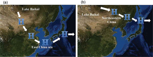
The other synoptic pattern (B type) is the case where a sounthern edge of low pressure system passes over the Korean peninsula. There were several cases where the Chinese PM assended and moved forward to the northeastern direction in warm sector of low pressure in Northern China, and flowed into the Korean peninsula while turning into the southeastern direction after being pushed by a strong cold air at the back of the cold front.

A type comprises 75% of the synoptic patterns while B type only 21%. Similarly, forecasters miss high PM events in A type by 75% while B type by 18%. Thus, no synoptic pattern might bias interpretation of high PM events.

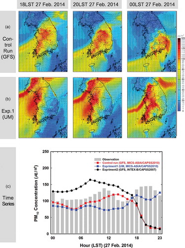
For the false forecasting events, when model output of both control run (GFS) and Exp. 1 (UM) is available, wind speed in control run is higher than in Exp. 1 while PM concentration is higher in Exp.1 than in control run as in Figure 6. Weak surface wind is likely to cause more stagnant air which is favorable for PM accumulation as seen in these cases. For example, the high PM event of February 27, 2014, was the case where the warm sector of the low pressure passed over the Korean peninsula. Forecasters miss this high PM event due to the modeling error in a surface wind. Figure 7a-b showed that apparently two PM plumes that originated from China were sequentially transported into the Korean peninsula on February 27. However, the moving speed of two plumes was quite dissimilar because the wind speeds simulated by control run and Exp.1 were quite different from each other. As shown in Figure 7c, This causes the difference in the ending time of the PM peaks in SMA. In control run, the peak dropped at the dawn of February 27, whereas in Exp. 1, the peak was maintained all-day long with the consecutive appearance of two peaks. Considering the existence of a significant difference between meteorological models, ensemble model rather than single model can have better performance in a real conditon.

Figure 6. Comparison of the simulated both PM₁₀ concentrations and surface wind speed in SMA for control run(GFS) and Exp. 1(UM).

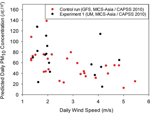
Figure 7. False forecasting case of February 27, 2014. Spatial distribution of the simulated PM₁₀ concentration for (a) control run and (b) Experiment 1; (c) daily variation of the observed PM₁₀ concentration in SMA with the simulated PM₁₀ concentration for control run, Experiment 1 and 2.

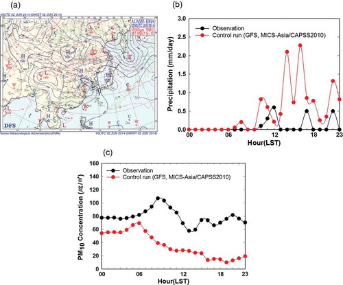
The error of the precipitation forecast is the second meteorological factor followed by the error of the surface wind forecast. This error usually occurs when the precipitation event is missed or when the precipitation amount is over-predicted. There were a total of six events of false forecasting caused by the incorrect precipitation, accounting for 43% of the false forecasts by the meteorological factor (14 events). The precipitation and PM concentration was mutually in inverse proportion due to the scavenging effect (not shown here) so that the error in quantitative precipitation forecast causes the the error in PM forecasting.

On June 02, 2015, precipitation occurred around southern Korea due to the low-level jet accompanied by the short wave trough at 850hPa (Figure 8). Control run predicted a precipitation of around 12mm at Seoul station, but in reality, there was only 2mm of precipitation. Consequently, CMAQ overestimated the scavenging effect resulting in the under-prediction of PM concentration in SMA.

Figure 8. False forecasting case of June 02, 2014. (a) 850hPa weather chart (source: KMA); (b) time series of the simulated and observed hourly precipitation; (c) hourly variation of the simulated and observed PM₁₀ concentration in SMA.

The forecast accuracy for PM in SMA between control run and Exp. 1 was compared in terms of AQL. For 24-h average PM₁₀, R² for control run and Exp. 1 are at a similar level, that is, 0.41 and 0.45, respectively. However, in terms of categorical statistics, their accuracies for PM₁₀ are similar (GFS: 67%, UM: 72%) under AQL of Normal, but at the AQL of Bad or above, the accuracy of Exp. 1 (41%) is more than two times higher than control run (17%). In other words, this result implies that, if the meteorological uncertainty is improved, the simulation capability for the high PM event can be further improved.

Uncertainty of the PM emission

Accuracy in emissions is critical to accuracy of PM forecast, together with that in the meteorological field. If the emission is insufficient or uncertain, the accuracy of forecast is directly deteriorated. Currently, the emission inventory in Northeast Asia is unlikely to catch up with the actual emission because of its rapid economic change (Woo et al., 2004). Furthermore, the actual situation of episodic emission sources, unexplainable information in inventories because it occurs irregularly and unpredictably such as fugitive/resuspended dusts and wildfires, is not precisely identified in this region. In addition, the profile information for spatial and temporal allocation, and chemical speciation for each emission source is not accurate to reflect these regional situations.

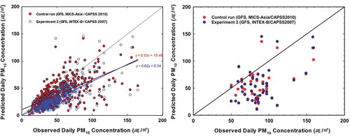
The emissions in Northeast Asia seem to be almost half explanative of the measured PM₁₀ concentration. The slopes of the simulated 24-h averaged PM₁₀ to measured one range from 0.5 to 0.6 as in Figure 9a during the evaluation period. The under-predictions of PM₁₀ in both control run and Exp. 2 are clearer in the false forecasting events as in Figure 9b with only a few over-predictions. The difference of simulated 24-h averaged PM₁₀ between two different emission models (control run and Exp.2) were just below 7 µg/m³ for the evaluation period. One of solutions is to reduce the time gap between the base year of emission inventory and real-time simulation by base year update or top-down emission since Northeast Asia countries undergo fast economic growth.

Figure 9. Comparison of observed and predicted 24-h average PM₁₀ concentration from control run(GFS, MICS-Asia/CAPSS2010) and Exp. 2(GFS, INTEX-B/CAPSS2007) during (a) the evaluation period and (b) all false forecasting cases.

The forecasting skill for PM_2.5 is overall better than that for PM₁₀. As in Table 5, NMBs and RMSEs for 24-h average PM_2.5 in both control run and Exp. 2 ranged from -20 to -25%, 25 to 27%, respectively, over SMA during all the year of 2014 while NMBs and RMSEs for 24-h average PM₁₀ in the both were the half ranging from -43 to -47% and 44 to 43%. The poorer forecasting skill for PM₁₀ than PM_2.5 reconfirmed the importance of missing episodic emission sources related with coarse particles.

Table 5. The comparison of forecasting accuracy in terms of PM₁₀ and PM_2.5 mass, and major PM_2.5 components depending on emission inventory when the forecasts were failed for 2014-year.

		PM10		PM2.5		Sulfate		OC		EC
		MC*	IC**	MC	IC	MC	IC	MC	IC	MC	IC
NMB	All	−42.8	−47.0	−20.3	−25.3	−35.3	−41.1	−33.9	−53.0	−10.2	−55.1
	False	−49.6	−47.9	−32.6	−31.7	−49.2	−45.0	−45.8	−60.2	−26.6	−66.5
MFB	All	−54.1	−64.1	−27.4	−38.7	−34.9	−45.4	−35.6	−67.3	−9.4	−67.4
	False	−67.9	−69.9	−43.2	−45.4	−65.7	−60.8	−55.6	−84.6	−36.0	−99.2
MFE	All	65.4	76.1	37.1	46.1	66.3	72.3	58.3	77.1	51.2	79.7
	False	74.9	80.6	50.7	56.4	86.1	85.5	68.1	86.5	58.2	99.4
RMSE	All	42.6	43.8	25.4	26.8	7.0	7.6	2.8	3.1	1.0	1.2
	False	68.2	68.3	46.1	49.7	13.6	14.4	5.3	5.6	1.7	2.1

Notes: *MC: MICS-Asia/CAPSS2010, ** IC: INTEX-B/CAPSS2007

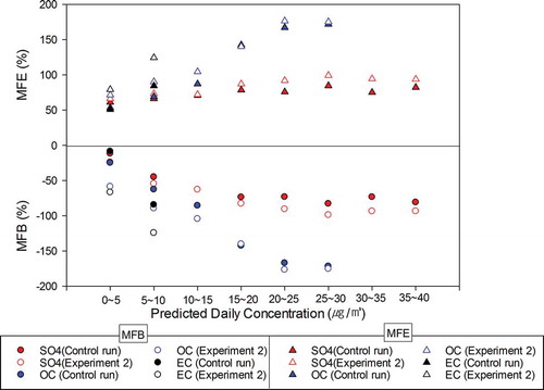
The under-predictions for PM₁₀ mass are also found for all major PM components as in Table 5. NMBs for sulfate, organic carbon (OC), and elemental carbon (EC) are -35.3%, -33.9%, and -10.2% respectively in the control run (MICS-ASIA/CAPSS2010) for the evaluation period when control run and Exp.2 are available. Meanwhile, the forecasting skills for PM components in control run is overall better than those in Exp. 2. For sulfate, OC and EC, Mean Fractional Bias (MFB) and Mean Fractional Error (MFE) in the control run are -35% and 66%, -36% and 58% and -9% and 51%, respectively while MFBs in Exp. 2 are -45% and 72%, -67% and 77%, -67% and 80%. The only use of MICS-ASIA/CAPSS2010 met the good performance criteria in terms of MFBs ≤±60% and MFEs ≤ 70% for major PM components recommended by Boylan and Russell (2006).

As the concentration level of PM components increase, MFBs for them also increase as in Figure 10 where the x-axis represents the 24 hour averaged concentration for sulfate, OC, and EC. MFB for sulfate approaches 100% as sulfate concentration increases while MFB for OC increases linearly with its concentration level. The pathway of secondary OC formation, accounting for substantial fraction of total organic particulate mass, is so uncertain that the OC underprediction becomes larger as pollution increases. The range of EC is below 10 ug/m³ in this study, and MFB /MFE in 5~10 ug/m³ is two times compared to in 0~5 ug/m³. It is shown that uncertainties of OC and EC increase along with concentration. It will be necessary to understand it in detail in future studies.

Figure 10. Mean fractional error (MFE) and mean fractional bias (MFB) for major components (Sulfate, OC, and EC) from control run (MICS-Asia) and Exp. 2(INTEX-B).

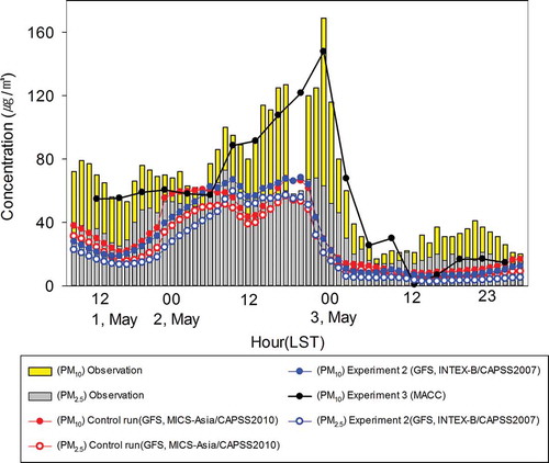
The false forecasting event on May 02, 2014, is likely due to missing coarse particle emission (Figure 11). While the low pressure located at Mongolia passed the northern part of the Korean peninsula, PM from northern China rapidly flowed into the Korean peninsula along the backside of the low pressure. Because of this, on May 02, the PM peak appeared in SMA for several hours and then disappeared. Both control run and Exp. 2 showed a large error in the start and the end of the peak as well as in the size of the peak. In particular, the negative bias in PM₁₀ was much larger than that in PM_2.5, which implies that an unidentified coarse particle emission source exists on the transport route. This has a thread of connection with the research result (Zhu et al., 2015) that there may be a significant emission of PM by the burning of agricultural residues in the northeastern part of China. According to Shi et al. (2014), the emission from burning contributed to 20-50% of the total PM10 with 50-100% optical depth in the major burning areas. The pollutants emitted from crop straw burning into the atmosphere in China can be transported even further across the boundaries to other countries. Furthermore, they informed that the total burned amount of agricultural residues may be the largest uncertainty source in emission estimation, because the portion of crop straw to be removed by burning used to be estimated based on historical rates. Therefore, it is considered that the main reason of unidentified coarse particle emission is from agricultural residues.

Figure 11. The comparison of the predicted PM from control run (MICS-Asia/CAPSS2010), Exp. 2(INTEX-B/CAPSS2007) and Exp. 3(MACC) concentrations with observations in the case of 2 May, 2014.

The data assimilation technique was investigated as the remedy against the emission uncertainty.

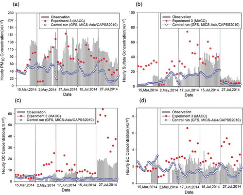
MACC showed better performance than CMAQ in SMA as in Figure 11, which was attributed to reflection of real-time Chinese PM into AQM. MACC reproduces an unidentified coarse particle better than CMAQ using prescribed emissions. This indicates that the forecasting skill for PM can be improved at SMA by better representing the long-range transport of PM by MACC.

However, MACC is not effective in PM component forecast. MACC reproduces PM₁₀ mass concentration but overpredicts major PM components at SMA as in Figure 12. One reason for the positive bias in sulfate, OC and EC is the superfluous allocation of satellite AOD into PM components because MACC does not contain a representation of ammonium nitrate (Giordano et. al., 2015).

Figure 12. The daily variation of the predicted and observed (a) PM₁₀ mass, (b) sulfate, (c) OC, and (d) EC on 15 March, 2 May, 17 June, 15 and 27 July in 2014 (Histogram: Observation, red dot: MACC, blue dot: CMAQ of control run).

To examine the overall performance of data assimilation on PM forecast, 15 cases, that the MACC and observation are available, were studied. As the results, the MACC has a better accuracy than CMAQ with a NMB of -31% and a RMSE of 40 µg/m³ (CMAQ with MICS-ASIA: NMB -35% RMSE 50 µg/m³). The NMB and RMSE of MACC and CMAQ are not much different from each other because MACC is a global model, and it cannot accurately simulate the local phenomenon compared to the long-range transport phenomenon.

AQM limit

The cases in AQM limit factor are remnants that are left over when all the false forecasting cases are categorized to the other three factors. In other word, they are the one that the three factors of meteorology, emission and forecaster are not able to explain the cause of false forecasting. Though the error in the initial and boundary conditions can cause false forecasting, at least the 5 events in the AQM limit factor showed no significant error in IC/BC. It might be that uncertainties in physical and chemical processes in AQM is the cause of AQM limit. As any single model has its own limit, ensemble forecast can offer a better forecast.

Lack of experience of the forecaster

The error of the forecaster occurs when he or she excessively depends on his or her past experience even though events are sometimes totally independent. The less experience a forecaster has in forecasting, the less experience he or she has for high PM events. In particular, the forecaster error occurred mainly on the next day of high PM events. For example, on the case of December 6, 2013, the forecasters decided that the high PM of ‘Bad’ level at December 5 would last to the next day, though the model prediction was ‘Normal’ level. One reason for this is the underprediction of the model on the previous high PM event day. Actually, the 24-h average observed PM concentration on December 6 dropped to 35.0 µg/m³ and the simulated PM concentration on the day was also low to 33.3 µg/m³. Because of the ventilation effect by the northwest wind, the high PM was cleared from the night of December 05.

Cause of false alarm

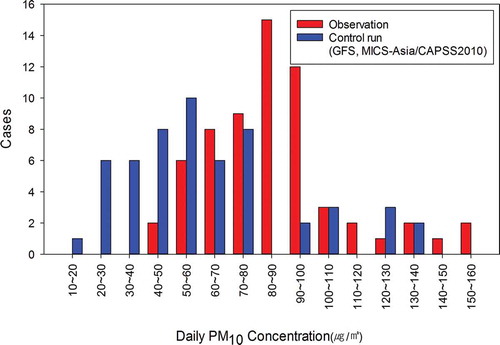
False alarm worsens the reliability of forecast as greatly as the forecast accuracy. As the result of collecting and analyzing all false alarm cases, we found that the reason for the false alarm was largely classified into three kinds: vicinity of AQL boundary, AQM over-prediction, and the error in forecasters’ decision-making. In particular, the vicinity of AQL boundary is the case when the actual observed PM concentration is concentrated around the AQL boundary. At this point, the model error is quite small. The false alarm of 74% was caused by not model but forecasters. Figure 13 shows the number of days when each simulated and observed PM occurred for all false alarm cases. A total of 55.6% of all false alarm cases was in the vicinity of observed AQL boundary (within 15% of boundary value of 80 µm/m³) between ‘Normal’ and ‘Bad’ level.

Figure 13. Comparison of the number of cases with 24-h average PM₁₀ for the false alarms between observation and model.

Summary

In this study, we introduced the air quality forecasting in Korea and investigated the causes of the false forecasting of PM. The forecasting accuracy of high PM event is mainly associated with the quality of AQM input of meteorology (25%) and emission (29%), and forecaster’s capacity (36%). Small difference in simulated wind speed between meteorology models led to larege difference in predicted PM concentration. Especially, under estimated surface wind cause more stagnant air which is favorable for PM accumulations. PM concentration is in inverse proportion to the precipitation so that the error of quantitative precipitation forecasting caused PM false forecasting by 9%. The emission inventories of INTEX-B, MICS-Asia and CAPSS used in this study were almost half explanative so that they might bias the interpretation of PM forecast systematically.

The PM forecast accuracy is at a decent level of 80%–90%, but the CSI is at a slightly lower level of 49%, which makes it necessary to conduct various improvements further to increase the forecasting accuracy.

Several scientific advances need to be taken to improve air quality forecasting. We updated the base year of the emission inventory and will further revise the Chinese emission data through projection by using Chinese real-time measurement network data, the top-down emission using environmental satellite data. In addition, we reflected more on the domestic meteorological characteristics by adopting the current KMA forecast model into NAGFMS. In the future, ensemble forecasting is considered, and a test bed for the super ensemble is being constructed. As is confirmed by Exp.3, AQM with MACC data for initial and boundary conditions is considered as one of the ensemble members. This is expected to improve the performance skill of CMAQ, especially, in the case of undefined coarse emission.

Furthermore, we plan to carry out forecast basis advancement, such as the construction of a web-based forecasting program that simultaneously display the forecast model results and domestic and foreign measurement data; the advancement of the comprehensive air quality information system for forecasters’ analysis and evaluation; and the extension of the air quality forecast modeling system hardware.

To strengthen the ability of forecasters, we establish a forecaster dispatch system to exchange forecast technology with forecast-operating countries and publish the casebooks that analyze the types of air pollution for forecasters.

To conclude, we conduct co-research through a Korea–China joint research team established at Beijing in June 2015, utilize top-down Northeast Asia emission data from the international program of MarcoPolo-Panda, and improve the air quality model by physical and chemical process study through carrying out a Korea–United States joint campaign for air quality study (KORUS-AQ) during May–June, 2016.

Additional information

Notes on contributors

Lim-Seok Chang

Lim-Seok Chang, Ara Cho, Hyunju Park, Kipyo Nam, Deokrae Kim, Ji-Hyoung Hong, and Chang-Keun Song work at the National Institute of Environmental Research in Incheon, Korea.

Ara Cho

Lim-Seok Chang, Ara Cho, Hyunju Park, Kipyo Nam, Deokrae Kim, Ji-Hyoung Hong, and Chang-Keun Song work at the National Institute of Environmental Research in Incheon, Korea.

Hyunju Park

Lim-Seok Chang, Ara Cho, Hyunju Park, Kipyo Nam, Deokrae Kim, Ji-Hyoung Hong, and Chang-Keun Song work at the National Institute of Environmental Research in Incheon, Korea.

Kipyo Nam

Lim-Seok Chang, Ara Cho, Hyunju Park, Kipyo Nam, Deokrae Kim, Ji-Hyoung Hong, and Chang-Keun Song work at the National Institute of Environmental Research in Incheon, Korea.

Deokrae Kim

Lim-Seok Chang, Ara Cho, Hyunju Park, Kipyo Nam, Deokrae Kim, Ji-Hyoung Hong, and Chang-Keun Song work at the National Institute of Environmental Research in Incheon, Korea.

Ji-Hyoung Hong

Lim-Seok Chang, Ara Cho, Hyunju Park, Kipyo Nam, Deokrae Kim, Ji-Hyoung Hong, and Chang-Keun Song work at the National Institute of Environmental Research in Incheon, Korea.

Chang-Keun Song

Lim-Seok Chang, Ara Cho, Hyunju Park, Kipyo Nam, Deokrae Kim, Ji-Hyoung Hong, and Chang-Keun Song work at the National Institute of Environmental Research in Incheon, Korea.

References

- Akimoto, H. 2003. Global air quality and pollution. Science. 302:1716–1719. doi:10.1126/science.1092666
- Amann, M., Z. Klimont, and F. Wagner. 2013. Regional and global emissions of air pollutants: Recent trends and future scenarios. Annu. Rev. Env. Resour. 38:31–55. doi:10.1146/annurev-environ-052912-173303
- Baklanov, A., A. Rasmussen, B. Fay, E. Berge, S. Finardi. 2002. Potential and shortcomings of numerical weather prediction models in providing meteorological data for urban air pollution forecasting. Water, Air and Soil Poll. 2(5–6):43–60. doi:10.1146/annurev-environ-052912-173303
- Boylan, J. W., and A. G. Russell. 2006. PM and light extinction model performance metrics, goals, and criteria for three-dimensional air quality models. Atmos. Environ. 40(26):4946–4959. doi:10.1016/j.atmosenv.2005.09.087
- Berge, E., S.–E. Walker, A. Sorteberg, M. Lenkopane, S. Eastwood, H. I. Jablonska, M. Ø. Koltzow. 2002. A real-time operational forecast model for meteorology and air quality during peak air pollution episodes in Oslo, Norway. Water, Air and Soil Pol. 2: 745–757. doi:10.1016/j.atmosenv.2005.09.087
- Byun, D. W., and J. K. S. Ching, Eds. 1999. Science algorithms for the EPA Model-3 Community Multiscale Air Quality (CMAQ) Modeling System. EPA-500/R-99/30.
- Carmichael, G. R., G. Calori, H. Hayami, et al. 2002. The MICS-Asia study: model intercomparison of long-range transport and sulfur deposition in East Asia. Atmos. Envion. 36(2):175–199. doi:10.1016/S1352-2310(01)00448-4
- Chan, F., and J. Duhia. 2001. Coupling and advanced land surface-hydrology model with the Penn State-NCAR MM5 modeling system Part I: model implementation and sensitivity. Mon. Weather Rev. 129:569–585. doi:10.1175/1520-0493(2001)129%3C0569:CAALSH%3E2.0.CO;2
- Chou, M.-D. and M.J. Suarez. 1999. A solar radiation parameterization for atmospheric studies. Technical report series on global modeling and data assimilation. NASA, TM-1999-104606(15).
- Dabberdt, W. F., M. A. Carroll, D. Baumgardner, et al. 2004. Meteorological research needs for improved air quality forecasting: Report of the 11th prospecus development team of the U.S. Weather Research Program. Bull. Amer. Meteor. Soc. 85:563–586. doi:10.1175/BAMS-85-4-563
- Davidson, C. I., R. F. Phalen, and P. A. Solomon. 2005. Airborne particulate matter and human health: A review. Aerosol Sci. Tech. 39(8):737–749. doi:10.1080/02786820500191348
- Giordano, L., D. Brunner, J. Flemming, et al. 2015. Assessment of the MACC reanalysis and its influence as chemical boundary conditions for regional air quality modeling in AGMEII-2. Atmos. Environ. 115:371–388. doi:10.1016/j.atmosenv.2015.02.034
- Guenther, A., T. Karl, P. Harley, et al. 2006. Estimates of global terrestrial isoprene emissions using MEGAN (Model of Emissions of Gases and Aerosols from Nature). Atmos. Chem. Phys. 6:3181–3210. doi:10.5194/acp-6-3181-2006
- Hemispheric Transport of Air Pollution (HTAP). 2010. Hemispheric Transport of Air Pollution 2010: Part A: Ozone and Particulate Matter, Air Pollution Studies no. 17, edited by: Dentener, F., Keating, T., and Akimoto, H., ECE/En.Air/100, ISSN 1014-4625, ISBN 978-92-1-117043-6.
- Hess, G.D., K.J. Tory, M.E. Cope, et al. 2004.The Australian air quality forecasting system. Part II: Case study of Sydney 7-day photochemical smog event. J. Appl. Meteorol. 43:663–679. doi:10.1175/2094.1
- Hong, S.-Y., H.–M. H. Juang, and Q. Zhao. 1998. Implementation of prognostic cloud scheme for a regional spectral model. Mon. Weather Rev. 126:2621–2639. doi:10.1175/1520-0493(1998)126%3C2621:IOPCSF%3E2.0.CO;2
- Hong, S.–Y., J. Dudhia, and S.–H. Chen. 2004. A revised approach to ice microphysical processes for the bulk parameterization of clouds and precipitation. Mon. Weather Rev. 132:103. doi:10.1175/1520-0493(2004)132<0103:ARATIM>2.0.CO;2
- Hong, S.-Y. and Y. Noh. 2006. A new vertical diffusion package with an explicit treatment of entrainment processes. Mon. Weather Rev. 134:2318–2341. doi:10.1175/MWR3199.1
- Houyoux, M. R. and J. M. Vukovich. 1999. Updates to the Sparse Matrix Operator Kernel Emission (SMOKE) modeling system and integration with Models-3. Environmental Programs MCNC, North Carolina Supercomputing Center, 3021 Cornwallis Road, Research Triangle Park, NC, 27709–2889.
- Inness, A., F. Baier, A. Benedetti, et al. 2013. The MACC reanalysis: an 8 yr data set of atmospheric omposition. Atmos. Chem. Phys. 13(8):4073–4109. doi:10.5194/acp-13-4073-2013
- Kain, J. S. 2004. The Kain-Fritsch convective parameterization: An update. J. Appl. Meteorol. 43: 170–181. doi:10.1175/1520-0450(2004)043%3C0170:TKCPAU%3E2.0.CO;2
- McKeen, S., S.H. Chung, J. Wilczak, et al. 2007. Evaluation of several PM2.5 forecast models using data collected during the ICARTT/NEAQS 2004 field study. J. Geophys. Res. 112:D10S20. doi:10.1029/2006JD007608.
- Michalakes, J., S. Chen, J. Dudhia, L. Hart, J. Klemp, J. Middlecoff, and Skamarock. 2001. Development of a next generation regional Weather Research and Forest model. Proceedings of the Ninth ECMWF Workshop on the Use of High Performance Computing in Meteorology. Eds. Walter Zwieflhofer and Norbert Kreitz, pp. 269–276. World Scientific: Singapore.
- Mlawer, E. J., S. J. Taubna, P. D. Brown, M. J. Lacono, and S. A. Clough. 1997. Radiative transfer for inhomogeneous atmospheres: RRTM, a validated correlated-k model for the longwave. J. Geophys. Res. 102. doi:10.1029/97JD00237
- Park, Y.- S., I.-S. Jang, S.-Y. Cho. 2015. An analysis on effects of the initial condition and emission on PM10 forecasting with data assimilation. J. KOSAE. 41(5):430–436. doi:10.5572/KOSAE.2015.31.5.430
- Phalen, R. F. and R. N. Phalen. 2011. Introduction to air pollution science. Jones & Bartlett Learning: Burlington, MA.
- Pope, C.A. III. 2000. What do epidemiologic findings tell us about health effects of environmental aerosols? J. Aerosols in Medicine. 13:335–354. doi:10.1089/jam.2000.13.335
- Schwartz, J., D.W. Dockery, and L.M. Neas. 1996. Is daily mortality associated specifically with fine particles? J. Air Waste Manag. Assoc. 46:927–939. doi:10.1080/10473289.1996.10467528
- Seaman, N.L. and S.A. Michelson. 2000. Mesoscale meteorological structure of a high ozone episode during the 1996 NARSTO-Northeast study. J. Appl. Meteorol. 39:384–398. doi:10.1175/1520-0450(2000)039<0384:MMSOAH>2.0.CO;2
- Seaman, N.L. 2003. Future direction of meteorology related to airquality research. Environ. Int. 20:245–252. doi:10.1016/S0160-4120(02)00183-6
- Seinfeld, J.H. and S.N. Pandis. 2006. Atmospheric chemistry and physics: From air pollution to climate change, second ed. John Wiley & Sons, Inc.: New York.
- Shi, T., Y. Liu, L. Zhang, Z. Gao. 2014. Burning in argricultural landscapes: an emerging natural and human issue in China. Landscape Ecol. 29(10):1785–1798.
- Stohl, A. and S. Eckhardt. 2004. Intercontinental transport of air pollution: an introduction. The Handbook of Environtal Chemistry. 4:G(1–11). doi:10.1007/b94521
- Thurston, G.D., K. Ito, C.G. Hayes, D.V. Bates, and M. Lippman. 1994. Respiratory hospital admissions and summer time haze air pollution in Toronto, Ontario: Consideration of the role of acid aerosol. Environ. Res. 65:271–290. doi:10.1006/enrs.1994.1037
- Woo, J.–H., J.M. Baek, J.–W. Kim, G.R. Carmichael, N. Thongboonchoo, S.T. Kim, J.H. An. 2004. Development of a multi-resolution emission inventory and its impact on sulfur distribution for Northeast Asia. Water, Air, and Soil Poll. 148(1):259–278.
- Woo, J.–H., K.-C. Choi, H.-K. Kim, B.-H. Baek, J.-H. Eum, C.-H. Song, Y.-I. Ma, Y. Sunwoo, L.-S. Chang, S.-H. Yoo. 2012. Development of an anthropogenic emissions percoessing system for Asia using SMOKE. W. Atmos. Environ. 58: 5–13. doi:10.1016/j.atmosenv.2011.10.042
- World Health Organization (WHO). 2004. Health aspects of air pollution, results from the WHO project “Systematic review of health aspects of air pollution in Europe.” June, E93090. World Health Organization: Copenhagen, Denmark.
- Zhang, Q., D.G. Streets, G.R. Carmichael, et al. 2009. Asian emissions in 2006 for the NASA INTEX-B mission. Atmos. Chem. Phys. 9:5131–5153. doi:10.5194/acp-9-5131-2009
- Zhang, Y., M. Bocquet, V. Mallet, C. Seigneur, and A. Baklanov. 2012a. Real-time air quality forecasting.Part I: History, techniques, and current status. Atmos. Environ. 50:632–655.
- Zhang, Y., M. Bocquet, V. Mallet, C. Seigneur, and A. Baklanov. 2012b. Real-time air quality forecasting, part II: State of the science, current research needs, and future prospects. Atmos. Environ. doi:10.1016/j.atmosenv.2012.02.041
- Zhu, C., K. Kawamura, and B. Kunwar. 2015. Effects of biomass burning over the western North Pacific Rim: Winter time maxima of an hydrosugas in ambient aerosols from Okinawa. Atmos. Chem. Phys. 15:1959–1973.doi:10.5194/acp-15-1959-2015