Trends and spatial patterns of fine-resolution aerosol optical depth–derived PM_2.5 emissions in the Northeast United States from 2002 to 2013

ABSTRACT

Clarifying the trends in quantity, location, and causes of PM_2.5 (particulate matter with an aerodynamic diameter <2.5 μm) emission changes is critical for evaluating and improving emission control strategies and reduce the risk posed to human health. According to the National Emissions Inventory (NEI) released by the U.S. Environmental Protection Agency (EPA), a general downward trend in PM_2.5 emissions has been observed in the United States over the past decade. Although this trend is representative at the national level, it lacks the precision to locate emission hotspots at a finer scale. Moreover, the changes reported in the NEI are likely confounded by periodic modification of inventory methods, and imprecision for area sources. In this regard, it is imperative to acquire emission inventories with as much spatial and temporal details as possible to further our knowledge of particle emissions, exposure levels, and associated health risks. In this study, we employed the PEIRS (Particle Emission Inventory using Remote Sensing) approach (Tang et al., 2016) predict triennial-averaged emissions at 1 km × 1 km resolution across the Northeast United States from 2002 to 2013. Notably, the PEIRS approach is able to capture both primary emission and secondary formation of PM_2.5. Regional emission trends were evaluated using quantile regression, and source-oriented trends were modeled with land use regression. The analysis found a regional decrease in PM_2.5 emissions of 3.3 tons/yr/km² (18%) over the 12-yr period. Furthermore, the rate of emission change at the extremes of the emission distribution was significantly different than that of the mean. Both quantile regression and spatial trends imply that the majority of the reduction in PM_2.5 emissions was attributable to highly developed spaces such as metropolitan areas and important traffic corridors. This urban-rural disparity was particularly apparent during the cold season. Indirect evidence suggested that the emission decline during the warm season is primarily attributed to less secondary particle formation. These findings warrant closer investigation of the impact of seasonality on PM_2.5 emissions.

Implications: Emission trend analysis provides crucial information for evaluating and enhancing the efficacies of emission control strategies as well as studying air pollution associated health risks. In this study, the patterns and trends of year-round and seasonal PM_2.5 emission over the Northeast United States are presented at a spatial resolution of 1 km × 1 km for the period of 2002–2012.

View correction statement:

Corrigendum

Introduction

Particulate matter with aerodynamic diameters less than 2.5 μm (PM_2.5) poses a serious public health concern. Globally, exposure to PM_2.5 contributed to approximately 3.5 million annual cardiopulmonary mortalities and 200,000 lung cancer–associated annual mortalities (Anenberg et al., 2010). In the United States (U.S.), an estimated 130,000 deaths per year were attributed to PM_2.5 exposure (Fann et al., 2012). Furthermore, a recent study reported that there is no safe threshold of PM_2.5 exposure (Shi et al., 2016). Thus, despite the significant decreases in PM_2.5 concentrations that have been achieved in the U.S. (Hu et al., 2013), there is a need to further improve air quality to reduce adverse health effects. The most effective way to improve air quality is through source control, and a better understanding of trends in the quantity, location, and causes of PM_2.5 emissions is of utmost importance to achieving this goal.

The U.S. Environmental Protection Agency (EPA), which is mandated to maintain good air quality for the general public, has taken a number of steps to monitor particle emissions over the past decade. Specifically, they developed the National Emissions Inventory (NEI) that contains triennially updated criteria (CAP) and hazardous (HAP) air pollutant emission estimates for a broad spectrum of source types. According to the 2011 NEI, primary anthropogenic PM_2.5 emission has decreased 53% nationally between 1990 and 2011, with the largest decline in the fuel combustion category (72%) (EPA, 2011). Typically, the East Coast shows the highest PM_2.5 emission density as well as its precursor gases, including sulfur dioxide (SO₂), volatile organic compounds (VOCs), and ammonia (NH₃). Most pollutants are generated in urban counties, except NH₃, which is higher in more rural areas where agricultural and pasture activities are frequent. Although the NEI trends are generally representative at the national level, local-scale emission characteristics are less clear because the NEI estimates are often based on county-level models using data collected at various points in time. Furthermore, the confluence of other air pollutants may also increase the uncertainty of local-scale models. For these reasons, EPA has sought more detailed analyses of local emission assessments.

EPA deploys a source-oriented approach to construct the NEI, which estimates the unit emission per activity (or emission factor) of known sources and acquires frequencies of the emission activities to predict total emissions. The NEI is useful in answering general emission questions over broad geographic areas, but this inventory method has led to several issues in interpreting emission trends. First, as EPA prioritizes tracking of primary particle sources, the NEI PM_2.5 emission estimates only represent a fraction of the total PM_2.5 emissions. Secondary particles are currently indirectly monitored by precursor gases that facilitate particle formations are only voluntarily reported. As secondary particles play an important role in the air quality in the U.S., more comprehensive measure or estimation on this portion of the pollution would render the NEI more complete. Second, whether the NEI trends reflect a real change or is merely a consequence of the periodic adjustment of inventory methodologies is still uncertain. A slight upward trend in PM_2.5 emissions from the highway vehicle sector was reported in both the 2005 NEI (EPA, 2005) and 2008 NEI (EPA, 2008). However, EPA scientists have concluded that the change is likely due to recent method and data improvements in estimating mobile sources (EPA, 2008). Lastly, updating new emission factors is costly and laborious. The prospect of comprehensively researching every existing and emerging emission source is unrealistic. Emission factors that are not regularly revised or updated may also lead to disparities in quality among source sectors. For instance, information on oil and gas operations was incomplete in the 2008 NEI, especially for non–point source sectors. The wide spread use of diesel engines to power hydraulic fracturing in the Marcellus shale and elsewhere means that emissions from individual wells may be underestimated (Natural Resources Defense Council [NRDC], 2014). Moreover, particle emissions from wildfires, prescribed fires, and biogenic sources are often excluded from the NEI due to high uncertainties of information. Since climate change is likely to increase the incidence of wildfires, this omission may produce misleading trends (EPA, 2016). Obsolete or incomplete emission information may render the NEI insufficient to accurately and comprehensively represent emission trends.

Instead of estimating individual emission factors, recently, we developed a new method (Particle Emission Inventories using Remote Sensing, PEIRS), which deploys a top-down approach by predicting the total PM_2.5 emissions directly using satellite data (Tang et al., 2016). Because satellite data have great potential to enhance the timeliness and locating accuracies for emission estimates, satellite imagery has been used to construct inventories for biomass burning or forest fire emissions (Zhang et al., 2011) and global aerosol emissions at 1°–2° spatial resolution (Dubovik et al., 2008; Huneeus et al., 2012). The PEIRS approach integrates state-of-the-art statistical modeling and long-term daily satellite retrievals of high-resolution 1 km × 1 km aerosol optical depth (AOD) data to generate spatially and time-resolved emission inventories. It has been successfully applied to predict 12-yr averaged emissions in the Northeast U.S., and the data have shown reasonable agreement with the county-level NEI. PEIRS emission estimates reflect small-scale intraurban variations, which provide crucial spatial information for health effects studies and legislative decision-making. More importantly, the PEIRS approach enables us to capture both primary emissions and secondary formation inside each 1 km × 1 km cell based on a mass balance model. The limitation of the PEIRS method is that AOD data retrieval is restricted during certain weather conditions (e.g., cloudy and snow covered days). However, the PEIRS can still provide ample temporal information when more than 1 yr of AOD data are used to predict emissions. Its enhanced cost-effectiveness and consistency also render the PEIRS inventory more adequate for trend analyses.

In this study, we applied the PIERS approach to estimate triennial-averaged PM_2.5 emission inventories and then assessed regional temporal and spatial trends in the Northeast U.S. (Figure 1). Calculation of multiyear emission averages is an interim strategy to compensate for weather-associated missing AOD data. Thus, our study duration consists of four 3-yr periods spanning from 2002 to 2013, which corresponds to the NEI triennial update schedule. Period 1 refers to 2002–2004, Period 2 to 2005–2007, Period 3 to 2008–2010, and Period 4 to 2011–2013. Regional emission trends were examined using quantile regression models, and source-oriented emission changes were predicted using land use regression. We applied the aforementioned analyses to (1) year-round, (2) warm season, and (3) cold season–specific emission estimates separately to further determine the seasonality of emission trends.

Figure 1. Study area: Northeast U.S.

Methods

Input data

Satellite AOD-derived PM_2.5 concentrations

We obtained spatially resolved daily PM_2.5 concentration estimates over the period from 2002 to 2013. The concentration estimates were derived from high-resolution (1 km × 1 km) daily AOD data from the Moderate Resolution Imaging Spectroradiometer (MODIS) instrument on board the Aqua Earth Observing Satellite. High-resolution AOD data were retrieved using the Multi-Angle Implementation of Atmospheric Correction (MAIAC) algorithm (Lyapustin et al., 2011), which has been proven to be more robust with higher retrieval rates (Chudnovsky et al., 2013). Detailed calibration procedures and performance are described in Tang et al. (2016).

Meteorological data

Daily averaged surface-level boundary layer height (PBL), temperature (TEMP), and wind field data during the period from 2002 to 2013 were obtained from the National Oceanic and Atmospheric Administration (NOAA) North America Regional Reanalysis (NARR) database (Mesinger et al., 2006). All NARR daily meteorological variables were linearly interpolated from the original resolution of 32 km × 32 km to a resolution of 1 km × 1 km using the scattered interpolant package from Mathworks (Natick, MA; http://www.mathworks.com/help/matlab/ref/scatteredinterpolant-class.html). After interpolating both wind field parameters into 1 km × 1 km resolution as described above, we calculated wind speed (WS) as the square root of sum of u² and v² and wind direction (WD) as the vector sum of u and v. We assumed that the daily wind direction and wind speed were constant within the boundary layer.

Land use variables

Land use parameters often serve as surrogates of anthropogenic PM_2.5 sources; in this study, land use parameters were used to quantify source-oriented emission intensities. The percentage of land cover in a grid of 1 km × 1 km cells covering the entire Northeast U.S. was obtained from the 2011 collection of the National Land Cover Database (NLCD). Important land cover parameters used in the land use regression (LUR) included spaces with high-, medium-, and low-intensity development, developed open spaces, agriculture, grass, deciduous forest, evergreen forest, and mixed forest. Major roads (A1–A3) density was gathered from the StreetMap USA database using the Feature Class Code (A1–A4) classification from the U.S. Census Bureau Topologically Integrated Geographic Encoding and Referencing (TIGER) system. Annual averaged traffic count for major roads was obtained from the Highway Performance Monitoring System (HMPS) database. The built-in Kernel density algorithm (Silverman, 1986) from ArcMap was used to calculate traffic count weighted for major road density within 1 km². Population density was calculated within 1 km² from the census track database of 2000. A variable indicating the presence of industrial point sources was created by intersecting the locations of large industrial facilities and the corresponding 1 km × 1 km cell in the study domain grid.

Statistical analysis

Emission model

PEIRS is an inventory method that models the dynamics of fine particle fate and transport on a gridded domain of 1 km × 1 km cells. Three central processes are accounted for in the PEIRS model: (1) transported particles from upwind to downwind cells, (2) within-cell emissions, and (3) particle removal by air exchange. The transport process closely depends on air exchange rate (α), which is a measure of the airflow entered or exitted from a fixed space. The volume of this fixed space in our study had a base area of 1 km × 1 km, and we used the boundary layer height (PBL, km) to estimate its height. The flow rate of this fixed volume of air was estimated by the produrct of horizontal wind speed (km/sec) and the cross-sectional area (PBL × 1 km) of the air movement. We obtained the air exchange rate, α (1/sec), as given in eq 1:

(1)

Once the air exchange rate was estimated for each grid cell daily, we then used wind direction to locate upwind cells that air masses carrying particles traveled through on the corresponding day. Additionally, temperature is included in the emission model as a surrogate for secondary particles formed outside of the downwind cell but not captured by the upwind concentrations. Detailed concepts and derivation of the emission model can be found in the previous study (Tang et al., 2016). The complete model (eq 2) is formulated as follows:

(2)

where C is the PM_2.5 concentrations in a downwind cell, C_ui is the PM_2.5 concentration in an upwind cell i, and Q is the estimated emission expressed in tons/yr/km². This model was fitted separately for each 1 km × 1 km grid cell across the Northeast U.S. to obtain Q.

Quantile regression

Emission trends were estimated using a linear quantile regression model with a linear variable indicating the time period (Period). Quantile regression has the advantage of estimating functional relationships for all portions of the emission distribution (e.g., percentiles) as opposed to the traditional mean estimator (Koenker and Bassett, 1978). In addition, quantile regression does not require any normality assumptions for variables. Quantile regression provides a more comprehensive analysis of the emission trends, specifically at the higher and lower percentiles in the distribution, where the trends in emissions may be quite different because those percentiles may have different source profiles from those that drive the center of the distribution of emissions. Quantile regression was performed from the 5th percentile to the 95th percentile using the quantreg package (version 5.26) (Koenker, 2015) in R version 3.2.2 (R Core Team, 2015).

Land use regression

Source-specific emissions and their trends were assessed using land use terms as predictors in the regression models. The land use parameters included percent developed spaces with high (dh), medium (dm), or low (dl) intensity, percent developed open spaces (dop), percent agricultural space (arg), percent deciduous forest (df), percent evergreen forest (ef), percent mixed forest (mf), traffic count weighted for major road density within 1 km² (rd), and population density within 1 km² (pop). In addition, we also created an indicator variable (ind) identifying the presence of major industrial sources in each 1 km × 1 km cell. Land use terms are surrogates for emissions and their relationship to emissions may change over time as, for example, pollution controls are implemented that impact the sources of those emissions. To test for these trends, we fitted four land use models separately for the four follow-up periods in the study due to the fact that some land use terms were only measured once over time. The four sets of slopes of the land use terms represent the emission intensity of the corresponding period, and the differences over follow-up periods represent their trends. The LUR model (eq 3) was formulated as follows:

(3)

where i is the study period, Q is the estimated emission, and the other predictors are as defined above. To test the significance of the LU-related emission trends (difference between slopes), we fitted the model below including emission estimates over the four study periods:

(4)

where k is the kth land use variable included in the LUR model (eq 4) and Period is a continuous variable of the period number.

Results and discussion

Regional and state-specific trends in PM_2.5 emissions

Regional PM_2.5 emission trends in the Northeast U.S. were estimated by comparing averages of year-round, cold season (November–April), and warm season (May–October) PEIRS emissions (Table 1). Across the entire study period (Period 4 vs. Period 1), year-round emissions decreased by 18%, which is comparable to the 11% decrease reported by the NEI during the period of 2002–2011 (EPA, 2011). The absolute reduction was more pronounced in the cold season, whereas the percentage decrease was larger in the warm season. The ratio of the regional mean emissions during the cold versus warm season also increased over time. These findings imply that current emission control is likely more effective in the warm season than the cold season. EPA scientists have similarly reported a generally lower effectiveness of emission controls during the winter due to strong weather interference on particle loading in the past decade (EPA, 2008).

Table 1. Regional PEIRS PM_2.5 mean triennial-averaged emissions over the four study periods.

	Mean emission (tons/yr/km^2)
Period	Year-round	Cold season	Warm season
Period 1 (2002–2004)	18.3	33.9	9.4
Period 2 (2005–2007)	17.4	31.1	7.3
Period 3 (2008–2010)	16.0	23.4	9.6
Period 4 (2011–2013)	15.0	26.4	4.4
	Mean emission changes (tons/yr/km^2, %)
	Year-round	Cold season	Warm season
Period 2 vs. 1	−0.9 (−5%)	−2.8 (−8%)	−2.1 (−22%)
Period 3 vs. 2	−1.4 (−8%)	−7.7 (−25%)	+2.3 (+32%)
Period 4 vs. 3	−1.0 (−6%)	+3.0 (+13%)	−5.2 (−54%)
Period 4 vs. 1	−3.3 (−18%)	−7.5 (−22%)	−5.0 (−54%)

The PEIRS emission trends varied by season and by location. Among seven Northeast U.S. states, Connecticut (CT) and Rhode Island (RI) exhibited the largest year-round PM_2.5 emission reduction during the study period (Table 2, Period 4 vs. Period 1). Furthermore, these two formerly nonattainment states exhibited a more than 20 tons/yr/km² decrease in PM_2.5 emissions during the cold season, which was almost twice that seen in the other five states. As the atmospheric conditions are less favorable for secondary particle formation during the cold season, the high-reduction rates observed in CT and RI during cold season is attributable to changes in primary emissions. The significant decrease in PM_2.5 emissions during the cold season began to manifest in Period 3 (2008–2010), after the nonattainment area designation in 2006 and before the maximum attainment in April 2010. This suggests that the states’ control programs for primary PM_2.5 emissions were effective. However, a number of factors may also contribute to this reduction. For instance, the demand for home heating oil in the Northeast fell by 43% between 2000 and 2012 and may have led to the declining emission during cold season (Andrews and Perl, 2014). Improved insulation, furnaces, and fuel switching from oil to gas may all play a role in addition to attainment designations. Furthermore, the observed reduction may be related to the economic recession during 2008 to 2010. People may tune down their thermostats lower to save money and lived in colder houses. This could also explain the increase in emission from Period 3 (2008~2010) to Period 4 (2011~2013) when the economy started recovering. On the other hand, the largest long-term reduction in PM_2.5 emissions during the warm season occurred in Vermont (VT; −9.3 tons/yr/km², −73%) followed by New Hampshire (NH; −8.7 tons/yr/km², −72%). Although drivers for the faster reduction rate in VT and NH during the warm season are unknown, the NEI reported larger percentage decreases in precursor gases (SO₂ and nitrogen oxides [NO_x]) than in primary PM_2.5 emissions in VT and NH during 2002–2011 (Table 3), which implies more rapid reduction in secondary particles than primary sources in less urbanized states.

Table 2. Regional PEIRS PM_2.5 mean triennial-averaged emission changes (tons/yr/km², %) by state.

Period	New York	Vermont	Massachusetts	Connecticut	New Hampshire	Maine	Rhode Island
Year-round
Period 2 vs. 1	−0.8 (−5%)	−2.2 (−13%)	+2.5 (+9%)	−2.7 (−9%)	−1.1 (−6%)	−0.7 (−4%)	+2.0 (+5%)
Period 3 vs. 2	−1.8 (−11%)	−1.6 (−11%)	−5.1 (−18%)	−0.4 (−1%)	−1.7 (−11%)	+1.0 (+6%)	−8.5 (−21%)
Period 4 vs. 3	+0.7 (+5%)	−1.7 (−12%)	−2.5 (−10%)	−5.8 (−20%)	−1.2 (−8%)	−2.7 (−17%)	−5.7 (−18%)
Period 4 vs. 1	−2.0 (−12%)	−5.5 (−32%)	−5.1 (−20%)	−8.8 (−28%)	−4.0 (−23%)	−2.5 (−15%)	−12.2 (−32%)
Warm season
Period 2 vs. 1	−0.9 (−12%)	−4.5 (−35%)	−1.0 (−9%)	−1.8 (−15%)	−5.2 (−43%)	−2.7 (−30%)	+0.3 (+2%)
Period 3 vs. 2	+1.4 (+20%)	+1.8 (+22%)	+2.4 (+23%)	+1.1 (+11%)	+3.6 (+52%)	+4.7 (+72%)	+1.0 (+8%)
Period 4 vs. 3	−4.0 (−50%)	−6.6 (−65%)	−6.9 (−54%)	−2.8 (−25%)	−7.2 (−68%)	−6.4 (−57%)	−5.9 (−41%)
Period 4 vs. 1	−3.6 (−47%)	−9.3 (−73%)	−5.6 (−49%)	−3.5 (−29%)	−8.7 (−72%)	−4.5 (−48%)	−4.6 (−36%)
Cold season
Period 2 vs. 1	−3.0 (−10%)	−2.8 (−10%)	+4.4 (+10%)	−4.9 (−9%)	+2.1 (+7%)	−7.4 (−21%)	+3.5 (+5%)
Period 3 vs. 2	−6.9 (−24%)	−7.2 (−27%)	−13.3 (−28%)	−8.2 (−16%)	−11.2 (−35%)	−5.3 (−19%)	−22.9 (−34%)
Period 4 vs. 3	+6.5 (+30%)	+2.0 (+10%)	−1.5 (−4%)	−11.2 (−26%)	+2.7 (+13%)	+0.3 (+1%)	−7.7 (−17%)
Period 4 vs. 1	−3.4 (−11%)	−8.0 (−27%)	−10.4 (−24%)	−24.4 (−43%)	−6.4 (−21%)	−12.3 (−35%)	−27.1 (−42%)

Table 3. NEI 10-year emission trends (%) for PM_2.5,* NO_x, SO₂, VOCs, and NH₃ in the Northeast U.S., 2002–2011.

Pollutant	New York	Vermont	Massachusetts	Connecticut	New Hampshire	Maine	Rhode Island
Year-round
PM2.5	−25% to −50%	−0% to −25%	−25% to −50%	−0% to −25%	−25% to −50%	−25% to −50%	+25% to +50%
NOx	−25% to −50%	−50% to −75%	−50% to −75%	−50% to −75%	−50% to −75%	−25% to −50%	−25% to −50%
SO2	−50% to −75%	−50% to −75%	−75% to −100%	−50% to −75%	−75% to −100%	−50% to −75%	−50% to −75%
VOCs	−25% to −50%	−0% to −25%	−25% to −50%	−25% to −50%	−25% to −50%	−25% to −50%	−0% to −25%
NH3	−0% to −25%	−0% to −25%	−25% to −50%	−25% to −50%	−0% to −25%	−0% to −25%	+50% to +75%

Note. PM_2.5 = particulate matter <2.5 μm diameter; NO_x = nitrogen oxides; SO₂ = sulfur dioxide; VOCs = volatile organic compounds; NH₃ = ammonia.

*NEI PM_2.5 consists of primary sources only.

Since the Emission Inventory System (EIS), a new tool with enhanced data collection approach than the past, was first used in the 2008 cycle (EPA, 2012), we were able to calculate the short-term trends of NEI between 2008 and 2011 and compare it with the PEIRS emission trends at corresponding periods (Periods 3–4; Table 4). Similar percent changes were observed in the states of New York, Vermont, and New Hampshire. The PEIRS trends show rapid reduction in Massachusetts, Connecticut, Maine, and Rhode Island, whereas the NEI trends exhibit less decrease or slight emission growth. We suspect that trend of secondary formation may result in the differences between the PEIRS and NEI trends. However, the underlying mechanisms of the disparities would require further investigation.

Spatial patterns and trends of PM_2.5 emissions

One of the advantages of satellite-based emission inventories is ample spatial information that allows visualization of the locations where reduction or growth occurred and consideration of appropriate emission control strategies. For year-round PM_2.5 emissions (Figure 2), urban areas such as the Greater Boston area and New York City exhibited a clear downward trend whereas rural trends were more difficult to determine. As discussed in the previous study (Tang et al., 2016), the PEIRS emission estimates in areas in the vicinity to water surfaces have larger uncertainties due to compromised AOD data. We observed potentially problematic emissions near Burlington, VT, due to interference from Lake Champlain. A similar problem occurred in Rochester, Syracuse, and areas bordering the Finger Lakes in New York. Relatively higher fraction of secondary particles involving complex reactions among precursor gases may provide another plausible explanation for the variations in emission trends in less urbanized areas. In particular, NH₃, NO_x, and VOC emissions were reported to be high in rural areas according to the 2011 NEI report (EPA, 2011). The NEI also found that significant reductions in NO_x, VOC, and SO₂ have been achieved over time whereas NH₃ emissions remained fairly constant. The uneven changes in these gas pollutants could modulate emission trends and spatial patterns significantly.

Figure 2. Year-round triennial-averaged PM_2.5 emission estimates during (a) Period 1, (b) Period 2, (c) Period 3, (d) Period 4 in the Northeast U.S. Cold season triennial-averaged PM_2.5 emission estimates during (e) Period 1, (f) Period 2, (g) Period 3, and (h) Period 4 in the Northeast U.S. Warm season triennial-averaged PM_2.5 emission estimates during (i) Period 1, (j) Period 2, (k) Period 3, and (l) Period 4 in the Northeast U.S.

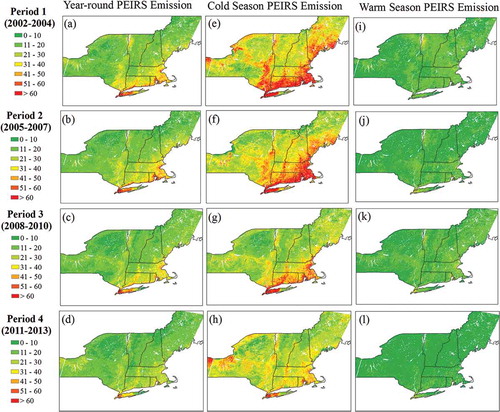
Cold season PM_2.5 emissions (Figure 2) generally showed similar spatial trends to those of the year-round emissions. In addition to the apparent decrease in emissions in metropolitan areas over time, reduction in important traffic corridors became more discernible during the cold season as well (i.e., Route 90 in the middle of the New York State). This indirectly supports the EPA inference that periodic method and data improvements used in the NEI are the main reasons for the observed increase in vehicle emissions in 2005 and 2008 NEI (EPA, 2008, 2011). In contrast, warm season PM_2.5 emissions (Figure 2) were distributed rather uniformly, with miniscule urban versus rural disparity. The onset of emissions reduction did not manifest during the warm season until the last period (2011–2013) measured. The difference between cold and warm season PM_2.5 emission trends implies a significant association between weather and total emissions and warrants further assessment of emission trends separately by season.

Quantile trends on PM_2.5 emission sources

To more closely investigate the large spatial variability of PM_2.5 emissions, we applied quantile regression models on emission inventories year-round (Figure 3a) and in the warm season (Figure 3b) and the cold season (Figure 3c) to quantify trends for a wider range of emission distribution. The quantile trend showed an exponential increase in the rate of reduction above the 80th percentile in year-round PM_2.5 emissions (Figure 3a). This result is consistent with our qualitative evaluation of the spatial trends (Figure 2) where reduction was most apparent in urban areas (higher quantile) and gradually tapered off in suburban and rural areas (lower quantile). The cold season quantile-specific trend was similar to that of the year-round quantile trend, but with larger deviance from the mean trend overall. This implies that urban-related PM_2.5 emission sources play an important role year-round but become considerably stronger in cold weather. On the other hand, the warm season quantile regression rate of change was similar throughout the distribution except for a weakening reduction rate below the 20th percentile, which, given how much lower emissions were in the warm season, represents areas that are quite clean already. The uniformity suggests little urban-rural contrast during the warm season, and that the warm season reduction is likely more attributable to sources that are not particularly urban-related, such as regional sources or secondary formation, which are expected to be more pronounced during warm season. This is in agreement with the state-specific trend where less urban states such as VT and NH showed the most reduction in PM_2.5 emissions during warm season (Table 3).

Figure 3. Quantile PM_2.5 emission trends (a) year-round and in the (b) warm season and (c) cold season in the Northeast U.S.

Trends in PM_2.5 emissions based on land use regression

Since the PEIRS emissions are not categorized by sources, we fitted land use regression models to categorize our emission inventory. Table 5 depicts the land use–specific PM_2.5 emission intensities over the four study periods. Over the entire study period, substantial reduction in PM_2.5 emissions was achieved across all land use–related sources. The year-round PEIRS emissions associated with developed spaces were estimated to reduce at the rate of 40–70% by the end of Period 4. This reduction rate was even more pronounced in the cold season (Table 6), due to reduced heating demands, specifically heating oil consumption (Andrews and Perl, 2014), as winter in the northeastern part of the U.S. have become warmer (Hayhoe et al., 2006) and efficiency of insulation and furnaces have also improved over the past decade. Land use–related PERIS emissions also decreased in the warm season in general except for high-intensity developed spaces, which almost tripled from Period 1 to Period 3 and then decreased sharply in Period 4 (Table 7). High-intensity developed spaces represent a mixture of land use, including commercial, industrial, and residential. The source profile for this geographic setting is complex; therefore, identifying the causes of this emission trend can be difficult. Regarding the transportation sector, emission from a vehicle that traveled 10,000 miles annually declined from an averaged year-round contribution of 1.58 to 0.98 tons/yr/km² over the past 12 yr (Table 5). Traffic-related PEIRS emission trends appeared to be consistent throughout the year with little seasonal variance. Furthermore, emissions from large industrial point sources such as power plants have declined despite the increasing energy demands. Population-related PEIRS emission fell substantially during cold season; however, during warm season, population input has little change over the decade—emission fell during the recession and then bounced back. Finally, for the forest categories, we found negative slopes in general, which indicates a net loss of particles due to more removal of PM_2.5 by plants, including interception and absorption (Nowak et al., 2013), than their biogenic emissions or resuspensions. The slopes of the forests, specifically deciduous forest, are more negative during cold season due to fewer or no leaves on the trees and thus less biogenic emissions (Megaritis et al., 2013). The land use regression results show that the removal mechanism of the forests became gradually stronger over the study period. However, since the removal mechanism may act synergistically with the weather, meteorological variations could be a confounding factor for the reduction observed in the forest categories.

Table 4. Percentage changes of PEIRS emissions from Period 3 to Period 4 and percentage changes of NEI emissions from 2008 to 2011.

Model	Period	New York	Vermont	Massachusetts	Connecticut	New Hampshire	Maine	Rhode Island
PEIRS (All seasons)	Period 4 vs. 3	+5%	−12%	−10%	−20%	−8%	−17%	−18%
NEI	2011 vs. 2008	+1%	−7%	+3%	+2%	−9%	−5%	−4%

Table 5. Land use-related PEIRS PM_2.5 emission intensities (tons/yr/km²) year-round in the Northeast U.S., 2002–2013.

Period	Intercept	Deciduous forest	Mixed forest	Evergreen forest	Agriculture/pasture	Industrial Points
Period 1 (2002–2004)	0.5*	−7.2*	−6.3*	−6.4*	0.1*	1.0*
Period 2 (2005–2007)	−3.7*	−5.5*	−4.5*	−5.7*	0.4*	1.7*
Period 3 (2008–2010)	7.2*	−9.5*	−5.3*	−8.2*	−0.1*	0.8*
Period 4 (2011–2013)	−1.3*	−10.2*	−8.6*	−10.7*	0.1*	0.5*
	Developed Open space	Developed High intensity	Developed Medium intensity	Developed Low intensity	Major road	Population
Period 1 (2002–2004)	27.3*	19.5*	23.4*	8.4*	9.8E-05*	4.05E-04*
Period 2 (2005–2007)	26.7*	23.2*	27.6*	9.2*	8.3E-05*	4.68E-04*
Period 3 (2008–2010)	20.3*	21.4*	20.7*	9.7*	8.4E-05*	4.88E-04*
Period 4 (2011–2013)	14.7*	11.3*	11.9*	2.5*	6.1E-05*	3.35E-04*

Note. Unit of the land use–related PEIRS emission intensity has a general form of tons/yr/km²/unit of land use.

Unit of land use variables:

1. % land cover inside 1 km × 1 km grid—Deciduous forest, Mixed forest, Evergreen forest, Agriculture/pasture, Developed open space, Developed high, medium, and low intensity

2. km × no. of vehicles inside 1 km × 1 km grid—Major Road

3. No. of person inside 1 km x 1 km grid—Population

*Statistically significant in the trend test.

Table 6. Land use–related PEIRS PM_2.5 emission intensities (tons/yr/km²) during the cold season (November–April) in the Northeast U.S., 2002–2013.

Period	Intercept	Deciduous forest	Mixed forest	Evergreen forest	Agriculture/pasture	Industrial points
Period 1 (2002–2004)	18.8*	−14.3*	−9.7*	−12.6*	−0.9	0.6*
Period 2 (2005–2007)	0.2*	−7.6*	−5.9*	−7.2*	+0.05	2.9*
Period 3 (2008–2010)	14.4*	−11.5*	−8.7*	−12.0*	+0.1	0.9*
Period 4 (2011–2013)	9.3*	−19.4*	−17.9*	−20.0*	+0.05	0.6*
	Developed Open space	Developed High intensity	Developed Medium intensity	Developed Low intensity	Major road	Population
Period 1 (2002–2004)	34.7*	21.3*	32.1*	9.7*	1.7E-04*	6.63E-04*
Period 2 (2005–2007)	38.0*	23.8*	39.2*	17.8*	1.4E-04*	4.78E-04*
Period 3 (2008–2010)	27.2*	23.9*	27.5*	11.4*	1.2E-04*	6.30E-04*
Period 4 (2011–2013)	8.9*	8.8*	5.5*	−0.7*	0.5E-04*	2.72E-04*

Note. Unit of the land use–related PEIRS emission intensity has a general form of tons/yr/km²/unit of land use.

Unit of land use variables:

1. % land cover inside 1 km × 1 km grid—Deciduous forest, Mixed forest, Evergreen forest, Agriculture/pasture, Developed open space, Developed high, medium, and low intensity

2. km × no. of vehicles inside 1 km × 1 km grid—Major Road

3. No. of person inside 1 km x 1 km grid—Population

*Statistically significant in the trend test.

Table 7. Land use–related PEIRS PM_2.5 emission intensities during the warm season (May-October) in the Northeast U.S., 2002–2013.

Period	Intercept	Deciduous forest	Mixed forest	Evergreen forest	Agriculture/pasture	Industrial points
Period 1 (2002–2004)	3.4*	-4.0*	0.5*	-0.7*	0.3*	0.7*
Period 2 (2005–2007)	1.4*	-4.5*	-3.0*	-3.1*	0.4*	0.1*
Period 3 (2008–2010)	6.1*	-7.8*	-1.4*	-4.3*	0.0*	0.8*
Period 4 (2011–2013)	0.6*	-4.5*	-2.8*	-4.5*	0.01*	-0.2*
	Developed Open space	Developed High intensity	Developed Medium intensity	Developed Low intensity	Major road	Population
Period 1 (2002–2004)	7.6*	3.4*	8.0*	4.2*	4.8E-05*	3.03E-04*
Period 2 (2005–2007)	8.8*	9.9*	10.9*	0.5*	1.4E-05*	2.20E-04*
Period 3 (2008–2010)	5.6*	11.8*	7.6*	2.6*	3.4E-07*	1.85E-04*
Period 4 (2011–2013)	6.5*	6.4*	5.2*	-1.2*	2.7E-05*	2.64E-04*

Note. Unit of the land use–related PEIRS emission intensity has a general form of tons/yr/km²/unit of land use.

Unit of land use variables:

1. % land cover inside 1 km × 1 km grid—Deciduous forest, Mixed forest, Evergreen forest, Agriculture/pasture, Developed open space, Developed high, medium, and low intensity

2. km × no. of vehicles inside 1 km × 1 km grid—Major Road

3. No. of person inside 1 km x 1 km grid—Population

*Statistically significant in the trend test.

Conclusions

In this paper, we constructed and analyzed the trends of satellite-based PM_2.5 emission inventories from 2002 to 2013 in the northeastern region of the U.S. PM_2.5 emissions in that region declined over the past 12 yr, with major reductions achieved for almost all land use–related sources. Results from the quantile regression results are in agreement with the spatial trends where most reductions were identified in urban areas or along important traffic corridors, particularly during the cold season. Seasonal variations in PM_2.5 emissions were distinguishable in all analyses performed in this study, and future efforts will continue to elucidate the underlying mechanisms for these seasonal differences in order to improve the efficacies of emission control strategies.

Acknowledgment

The authors especially thank Joy Lawrence and Stacey Tobin for their comments and review of drafts.

Funding

This publication was made possible by the U.S. Environmental Protection Agency (EPA) grant RD83479801 and the ACE grant RD-835872-01. Its contents are solely the responsibility of the grantee and do not necessarily represent the official views of the EPA. Further, the EPA does not endorse the purchase of any commercial products or services mentioned in the publication.

Additional information

Funding

This publication was made possible by the U.S. Environmental Protection Agency (EPA) grant RD83479801 and the ACE grant RD-835872-01. Its contents are solely the responsibility of the grantee and do not necessarily represent the official views of the EPA. Further, the EPA does not endorse the purchase of any commercial products or services mentioned in the publication.

Notes on contributors

Chia-Hsi Tang

Chia-Hsi Tang is a doctoral student of the Department of Environmental Health at Harvard School of Public Health.

Brent A. Coull

Brent A. Coull is a professor of the Department of Biostatistics at Harvard School of Public Health.

Joel Schwartz

Joel Schwartz is a professor of the Department of Environmental Health at Harvard School of Public Health.

Qian Di

Qian Di is a doctoral student of the Department of Environmental Health at Harvard School of Public Health.

Petros Koutrakis

Petros Koutrakis is a professor of the Department of Environmental Health at Harvard School of Public Health.

References

- Andrews, A., and L. Perl. 2014. The Northeast Heating Oil Supply, Demand, and Factors Affecting Its Use, ed. Committees of Congress. Washington, DC: U.S. Government Printing Office.
- Anenberg, S.C., L.W. Horowitz, D.Q. Tong, and J.J. West. 2010. An estimate of the global burden of anthropogenic ozone and fine particulate matter on premature human mortality using atmospheric modeling. Environ. Health Perspect. 118:1189–1195. doi: 10.1289/ehp.09-01220.
- Chudnovsky, A., C. Tang, A. Lyapustin, Y. Wang, J. Schwartz, and P. Koutrakis. 2013. A critical assessment of high-resolution aerosol optical depth retrievals for fine particulate matter predictions. Atmos. Chem. Phys. 13:10907–10917. doi: 10.5194/acp-13-10907-2013.
- Dubovik, O., T. Lapyonok, Y.J. Kaufman, M. Chin, and P. Ginoux. 2008. Retrieving global aerosol sources from satellites using inverse modeling. Atmos. Chem. Phys. 8:250. doi:10.5194/acp-8-209-2008.
- Fann, N., A.D. Lamson, S.C. Anenberg, K. Wesson, D. Risley, and B.J. Hubbell. 2012. “Estimating the national public health burden associated with exposure to ambient PM2.5 and ozone. Risk Anal. 32:81–95. doi: 10.1111/j.1539-6924.2011.01630.x.
- Hayhoe, K., C.P. Wake, T.G. Huntington, L. Luo, M.D. Schwartz, J. Sheffield, E. Wood, B. Anderson, J. Bradbury, A. DeGaetano, T.J. Troy, and D. Wolfe. 2006. Past and future changes in climate and hydrological indicators in the US Northeast. Climate Dyn. 28:381–407. doi: 10.1007/s00382-006-0187-8.
- Hu, X., L.A. Waller, A. Lyapustin, Y. Wang, and Y. Liu. 2013. 10 yr spatial and temporal trends of PM2.5 concentrations in the southeastern US estimated using high-resolution satellite data. Atmos. Chem. Phys. Discuss. 13:25617–25648. doi: 10.5194/acpd-13-25617-2013.
- Huneeus, N., F. Chevallier, and O. Boucher. 2012. Estimating aerosol emissions by assimilating observed aerosol optical depth in a global aerosol model. Atmos. Chem. Phys. 12:4585–4606. doi: 10.5194/acp-12-4585-2012.
- Koenker, R. 2015. Quantile regression in R: A vignette. https://cran.r-project.org/web/packages/quantreg/vignettes/rq.pdf
- Koenker, R., and G. Bassett. 1978. Regression quantiles. Econometrica 46:33–50. doi: 10.2307/1913643.
- Lyapustin, A., Y. Wang, I. Laszlo, R. Kahn, S. Korkin, L. Remer, R. Levy, and J.S. Reid. 2011. Multiangle implementation of atmospheric correction (MAIAC): 2. Aerosol algorithm. J. Geophys. Res. 116(D3):D03211. doi: 10.1029/2010jd014986.
- Megaritis, A.G., C. Fountoukis, P.E. Charalampidis, C. Pilinis, and S.N. Pandis. 2013. Response of fine particulate matter concentrations to changes of emissions and temperature in Europe. Atmos. Chem. Phys. 13:3423–3443. doi: 10.5194/acp-13-3423-2013.
- Mesinger, F., G. DiMego, E. Kalnay, K. Mitchell, P.C. Shafran, W. Ebisuzaki, D. Jović, J. Woollen, E. Rogers, E.H. Berbery, M.B. Ek, Y. Fan, R. Grumbine, W. Higgins, H. Li, Y. Lin, G. Manikin, D. Parrish, and W. Shi. 2006. North American regional reanalysis. Bull. Am. Meteorol. Soc. 87:343–360. doi: 10.1175/bams-87-3-343.
- Nowak, D.J., S. Hirabayashi, A. Bodine, and R. Hoehn. 2013. Modeled PM2.5 removal by trees in ten U.S. cities and associated health effects. Environ. Pollut. 178:395–402. doi: 10.1016/j.envpol.2013.03.050.
- Natural Resources Defense Council. 2014. Fracking fumes: Air pollution from hydraulic fracturing threatens public health and communities. https://www.nrdc.org/sites/default/files/fracking-air-pollution-IB.pdf
- R Core Team. 2015. R: A Language and Environment for Statistical Computing [computer software]. Vienna, Austria: R Foundation for Statistical Computing. http://www.R-project.org/ (accessed October 3, 2016).
- Shi, L., A. Zanobetti, I. Kloog, B.A. Coull, P. Koutrakis, S.J. Melly, and J.D. Schwartz. 2016. Low-concentration PM2.5 and mortality: Estimating acute and chronic effects in a population-based study. Environ. Health Perspect. 124:46–52. doi: 10.1289/ehp.1409111.
- Silverman, B. 1986. Density Estimation for Statistics and Data Analysis. New York: Chapman and Hall.
- Tang, C., B.A. Coull, J Schwartz, A. Lyapustin, Q. Di, and P. Koutrakis. 2016. Developing Particle Emission Inventories Using Remote Sensing (PEIRS). J. Air Waste Manage. Assoc. doi: 10.1080/10962247.2016.1214630.
- U.S. Environmental Protection Agency. 2005. 2005 National Emissions Inventory Data & Documentation. https://www.epa.gov/sites/production/files/2015-11/documents/nei_point_2005_9-10.pdf
- U.S. Environmental Protection Agency. 2008. 2008 National Emissions Inventory: Review, Analysis and Highlights. https://www.epa.gov/sites/production/files/2015-07/documents/2008_neiv3_tsd_draft.pdf
- U.S. Environmental Protection Agency. 2011. Profile of the 2011 National Air Emissions Inventory. https://www.epa.gov/sites/production/files/2015-08/documents/lite_finalversion_ver10.pdf
- U.S. Environmental Protection Agency. 2012. Evaluate 2008 NEI to identify areas of improvement that benefit use in residual risk assessments. https://www.epa.gov/sites/production/files/2015-07/documents/evaluate2008nei_rtr_finalreport20121220.pdf
- U.S. Environmental Protection Agency. 2016. Climate change indicators in the United States: Wildfires. https://www.epa.gov/sites/production/files/2016-08/documents/climate_indicators_2016.pdf
- Zhang, J.H., F.M. Yao, C. Liu, L.M. Yang, and V.K. Boken. 2011. Detection, emission estimation and risk prediction of forest fires in China using satellite sensors and simulation models in the past three decades—An overview. Int. J. Environ. Res. Public Health 8:3156–3178. doi: 10.3390/ijerph8083156.