Expected ozone benefits of reducing nitrogen oxide (NO_x) emissions from coal-fired electricity generating units in the eastern United States

ABSTRACT

On hot summer days in the eastern United States, electricity demand rises, mainly because of increased use of air conditioning. Power plants must provide this additional energy, emitting additional pollutants when meteorological conditions are primed for poor air quality. To evaluate the impact of summertime NO_x emissions from coal-fired electricity generating units (EGUs) on surface ozone formation, we performed a series of sensitivity modeling forecast scenarios utilizing EPA 2018 version 6.0 emissions (2011 base year) and CMAQ v5.0.2. Coal-fired EGU NO_x emissions were adjusted to match the lowest NO_x rates observed during the ozone seasons (April 1–October 31) of 2005–2012 (Scenario A), where ozone decreased by 3–4 ppb in affected areas. When compared to the highest emissions rates during the same time period (Scenario B), ozone increased ∼4–7 ppb. NO_x emission rates adjusted to match the observed rates from 2011 (Scenario C) increased ozone by ∼4–5 ppb. Finally in Scenario D, the impact of additional NO_x reductions was determined by assuming installation of selective catalytic reduction (SCR) controls on all units lacking postcombustion controls; this decreased ozone by an additional 2–4 ppb relative to Scenario A. Following the announcement of a stricter 8-hour ozone standard, this analysis outlines a strategy that would help bring coastal areas in the mid-Atlantic region closer to attainment, and would also provide profound benefits for upwind states where most of the regional EGU NO_x originates, even if additional capital investments are not made (Scenario A).

Implications: With the 8-hr maximum ozone National Ambient Air Quality Standard (NAAQS) decreasing from 75 to 70 ppb, modeling results indicate that use of postcombustion controls on coal-fired power plants in 2018 could help keep regions in attainment. By operating already existing nitrogen oxide (NO_x) removal devices to their full potential, ozone could be significantly curtailed, achieving ozone reductions by up to 5 ppb in areas around the source of emission and immediately downwind. Ozone improvements are also significant (1–2 ppb) for areas affected by cross-state transport, especially Mid-Atlantic coast regions that had struggled to meet the 75 ppb standard.

Introduction

The 2008 National Ambient Air Quality Standard (NAAQS) for surface ozone is a daily maximum 8-hr average of 75 ppb (U.S. Environmental Protection Agency [EPA], 2008). Regions failing to meet this standard are designated as nonattainment areas (NAAs) and required to submit a State Implementation Plan (SIP) to outline regulatory measures that would result in attainment (EPA, 2015a). In October 2015, a stricter ozone NAAQS was mandated, lowering the 8-hr standard to 70 ppb (EPA, 2015b).

Surface ozone is formed most abundantly in the presence of volatile organic compounds (VOCs) and nitrogen oxides (NO_x; nitric oxide [NO] + nitrogen dioxide [NO₂]) during hot, sunny summer days (Crutzen, 1974; Haagensmit et al., 1953). One significant source of NO_x comes from electricity generating units (EGUs) that often run heavily to meet demand for air conditioning on hot summer days in the United States (U.S.). EGUs also have smokestacks that emit at elevated heights and allow for long-range transport of pollutants. Various regulations such as the recent Cross-State Air Pollution Rule (EPA, 2015c) have been implemented to limit emissions in one state that could adversely affect another downwind state.

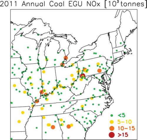
During the summer, the Bermuda high, a high pressure system that can last several consecutive days, often moves westward to a position off the Mid-Atlantic coast, and the anticyclonic flow promotes transport of emissions from sources along the Ohio River and in Pennsylvania into Mid-Atlantic and northeastern states (Hains et al., 2008; He et al., 2013a, 2013b, 2014; Ryan et al., 1998; Smith and Tirpak, 1988; Taubman et al., 2004, 2006). Figure 1 shows that most of the largest coal-fired EGU NO_x emitters in the eastern U.S. are located in these regions upwind of the East Coast, based on 2011 reported emissions (EPA, 2015d), and emissions from EGUs can have substantial impacts on downwind air quality (He, 2013a).

Figure 1. Total annual emissions of NO_x (in units of thousands of metric tons NO₂ equivalent) from coal-fired EGUs at the facility level as reported in 2011 to the Clean Air Markets Division (CAMD) (EPA, 2015d).

An analysis of 2005–2007 Ozone Monitoring Instrument (OMI) NO_x satellite observations found ozone production in most of the U.S. was sensitive to concentrations of NO_x, and more so at higher temperatures (Duncan et al., 2010), making summertime NO_x critical to ozone formation. Similarly, Comprehensive Air Quality Model with Extensions (CAMx) modeling results for July 2011 also indicated ozone formation in and around the state of Maryland to be almost exclusively NO_x-sensitive (Goldberg et al., 2016). This has been a result of reducing local sources of NO_x, such as cleaner motor vehicles and power plants (Duncan et al., 2010). Further NO_x emission reductions will produce direct ozone decreases, but increased NO_x would have adverse effects.

Although many EGUs have recently switched to natural gas as a fuel source, coal remains an equally important source for electricity in the U.S., with both fuel sources used to produce roughly a third of total generated electricity each in 2015; other nonrenewable fuels contributed less than 1% (U.S. Energy Information Administration [EIA], 2016). Although natural gas power plants emit NO_x, coal-fired units emit, on average, 4 times as much on a mass/MWhr basis (Roy and Choi, 2015). One effective method of reducing NO_x emissions from coal-fired power plants is the use of devices such as selective catalytic and noncatalytic reduction (SCR and SNCR, respectively) following the combustion process, which can eliminate up to 90% and 50%, respectively, of produced NO_x (EPA, 2003a, 2003b).

Under federal regulations, EGU operators are mandated to keep NO_x emissions under an allotted amount, based on a given state’s emissions budget (EPA, 2016), and installation of SCR or SNCR is often needed to meet the requirement. As long as the unit’s annual and ozone season emissions caps are not exceeded, current rules and regulations allow for these controls to be shut off to limit fiscal burden. Once the capital investment has been made to install such controls, the cost of chemical reagent and efficiency reductions are the only major maintenance and operational costs (EPA, 2015e), yet emissions monitors indicate that these controls are not always being utilized to their fullest potential (EPA, 2015e, 2015f; He et al., 2013b).

McNevin (2016) reported that over the past few years, the degree of usage of installed SCR units has dropped substantially at individual plants in the eastern US, and pointed out the need to ensure optimal use of NO_x control technology. An investigation of average ozone season NO_x emission rates from coal-fired EGUs in the eastern U.S. revealed several units where rates increased from 2004 to 2014. This trend suggested that unit owners and operators found it cost-effective to limit operations of SCR or SNCR systems and instead use lenient regulatory or market mechanisms to legally meet their caps (Ozone Transport Commission [OTC], 2015). This increase in NO_x emissions from not utilizing postcombustion controls can lead to increased ozone production locally and downwind. Alternatively, operating these controls at optimal rates could decrease ozone concentrations. Using a chemical transport model, we quantify the regional impacts of EGU NO_x controls on ozone formation.

Model description

The EPA provided state agencies with air quality model-ready surface emission estimates (EPA’s ed_v6_11f modeling case) for 2011 and estimated emissions for 2018, based on the 2011 National Emissions Inventory (NEI) (EPA, 2014a). The 2018 emission estimates reflect planned “on-the-books” controls and regulations such as more efficient technologies and fuel usage for vehicles and facilities, but they do not include additional measures needed for attainment of the 2008 ozone NAAQS. We used the Sparse Matrix Operator Kernel Emissions (SMOKE) System version 3.1 (SMOKE, 2012) to process plume rise for elevated point source inventories, such as EGUs, and to combine them with the surface emissions. These emissions included the Biogenic Emission Inventory System (BEIS) version 3.14 for biogenic sources (2011 emissions were used for both 2011 and 2018), Motor Vehicle Emission Simulator (MOVES) 2010b for mobile sources, and the Integrated Planning Model (IPM) version 5.13 for the EGU sources.

These emissions processed by SMOKE were then input into to the Community Multi-scale Air Quality (CMAQ) version 5.0.2, a model which also incorporates meteorological data and chemical reaction kinetics to calculate expected formation and dispersion of various pollutant species (CMAQ, 2015; Foley et al., 2010). The CMAQ simulations have 12 km × 12 km horizontal grid resolution, 34 layer sigma-coordinate vertical levels (from surface to ~20 km), and hourly output for an eastern U.S. modeling domain. Meteorological fields for 2011 were generated using the Weather Research and Forecasting (WRF) version 3.4 model (EPA, 2014b) and further processed through the Meteorology-Chemistry Interface Processor (MCIP) to prepare the meteorology fields for use in CMAQ. To limit the impacts of initial conditions on model results, 14 days of model spin-up were used. Boundary conditions were supplied by GEOS-Chem version 8-03-02 (Bey et al., 2001), and version 5 of the Chemical Bond mechanism with updates to toluene and chlorine chemistry (CB05TUCl) (Sarwar et al., 2012) was used with AE6 scheme for aerosols (Appel et al., 2013; Nolte et al., 2015). Plume-in-grid treatment was not used for the EGUs in this study, but similar results for modeled ozone would be expected, with impacts reaching even farther downwind (Karamchandani et al., 2014).

Methods

To determine and quantify the impact of NO_x emissions from coal-fired EGU sources on surface ozone concentrations, baseline runs for July 2011 and 2018, and four sensitivity scenarios for 2018 were performed by adjusting EGU NO_x emission rates based on historical records. For both 2011 and 2018, while emissions were varied, meteorology for July 2011 was held constant throughout to remove the influence of meteorological conditions on model results. The 2011 Baseline and 2018 Baseline were run using EPA-approved emissions, with the sensitivity scenarios building off of the 2018 Baseline emissions.

The Clean Air Markets Division (CAMD) of the EPA supports several regulatory programs that require continuous monitoring of large point-source emissions of sulfur dioxide (SO₂) and NO_x (EPA, 2015d). CAMD NO_x emission data were obtained (available for download from https://ampd.epa.gov/ampd/) for the ozone seasons during the years of 2005 through 2012 and analyzed for the states of Illinois, Indiana, Kentucky, Maryland, Michigan, North Carolina, Ohio, Pennsylvania, Tennessee, Virginia, and West Virginia. Rates can vary from unit to unit depending on multiple factors, such as installed controls, sequence of controls, gas temperature (which affects efficiency), and operational load. To capture some of these concerns, we use the average ozone season rates for each individual unit instead of simply applying only a single rate to every unit. The lowest, highest, and 2011 ozone season average NO_x emission factors (lb/MMBTU) were found for each individual coal-fired unit equipped with SCR or SNCR controls.

The average ozone season historical CAMD NO_x emission rates for each coal-fired unit from each year from 2005 through 2012 were compared with the rates from the 2018 IPM inventory files. For each unit, the ratio between lowest historical NO_x rates and 2018 IPM NO_x rates was calculated and used as a multiplier that was applied to the hourly and annual IPM emissions inventory files and reprocessed through the SMOKE model. These new EGU emissions representing coal-fired units operating at their lowest rates were combined with the other 2018 emissions to create 2018 Scenario A.

Using a similar approach, NO_x rates for coal-fired units were instead increased to represent operation at the highest historical rates in 2018 Scenario B. In 2018 Scenario C, NO_x emissions were increased to match the observed 2011 emission rates from coal-fired units, with emission projections for 2018 in all other sectors remaining unchanged. Finally, 2018 Scenario D has units operating at lowest NO_x rates (Scenario A), and additionally includes SCR NO_x reductions for the 2018 EGUs that are expected to lack postcombustion controls. To assume SCR reductions on uncontrolled units in Scenario D, a multiplier was calculated for each unit by dividing the 2018 ozone season emission rate by the state-averaged SCR-controlled lowest average ozone season emission rate. The unit-specific reductions applied for each scenario are provided in Table S2, and a summary of the model scenarios is provided in Table 1.

Table 1. Brief descriptions of the modeling scenarios.

Scenario	Brief description
2011 Baseline	2011 EPA-provided emissions were used with no modifications.
2018 Baseline	2018 EPA-provided, projected emissions were used with no modifications.
2018 Scenario A	2018 SCR/SNCR EGU NOx emissions are reduced to match lowest rates observed in 2005–2012 historical data.
2018 Scenario B	2018 SCR/SNCR EGU NOx emissions are reduced to match highest rates observed in 2005–2012 historical data.
2018 Scenario C	2018 SCR/SNCR EGU NOx emissions are increased to match rates observed in 2011. Emission projections for 2018 in all other sectors remain unchanged.
2018 Scenario D	2018 SCR/SNCR EGU NOx emissions are reduced to match lowest rates observed in 2005–2012 historical data and 2018 EGUs lacking postcombustion controls modeled to include SCR NOx reductions.

A comparison of the annual NO_x emissions for all EGUs in the eastern U.S. from each of these scenarios can be seen in Table 2. The largest reductions occur in Scenario D, followed by Scenario A. Even with NO_x emissions increased from the 2018 Baseline, Scenarios B and C still have lower emissions than what is shown for 2011. This is a result of unit shutdowns, fuel-switching, and additional controls between 2011 and 2018, and that only select coal-fired EGUs were adjusted for these scenarios (Table S2), leaving other coal-fired units, as well as units powered by other fuel sources, unchanged. Reported values for the eastern U.S. include the western borders of Texas, Oklahoma, Kansas, Nebraska, South Dakota, and North Dakota and all states eastward.

Table 2. 2011 and 2018 anthropogenic annual eastern U.S. EGU NO_x emissions (in tons).

Emission	2011 Baseline	2018 Baseline	2018 Scenario A	2018 Scenario B	2018 Scenario C	2018 Scenario D
Total annual EGU NOx (tons)	1,695,870	1,262,505	1,117,819	1,437,663	1,302,481	1,053,253
Percent change from 2011	—	−26%	−34%	−15%	−23%	−38%
Percent change from 2018	+34%	—	−11%	+14%	+3%	−17%

From 2011 to 2018, various sectors are expected to see reductions of anthropogenic NO_x emissions (Table 3), as well as anthropogenic VOC emissions (Table S1). The largest NO_x reductions come from the on-road and nonroad sources, with sizeable reduction percentages from EGUs as well as locomotives and marine vessels. Oil and gas sector emissions included in the inventory are projected to significantly increase to future year 2018. Overall for the eastern U.S. when compared with 2011, anthropogenic emissions of NO_x are forecasted to be down 29% and VOCs by 11% (EPA, 2014c).

Table 3. 2011 and 2018 annual eastern U.S. anthropogenic NO_x emissions (in tons) by sector.

Emission source	2011 Baseline	2018 Baseline	Percent change
Area	707,844	720,594	+2%
Nonroad	1,337,283	867,419	−35%
On-road	4,476,491	2,031,596	−55%
EGU point sources	1,695,870	1,262,505	−26%
Other point sources	1,457,899	1,452,572	−0%
Oil and gas extraction	557,911	684,604	+23%
Locomotive and marine vessels	911,521	760,914	−17%
Residential wood combustion	27,349	29,839	+9%
Fire	246,027	246,027	0%
Total	11,418,195	8,056,069	−29%

Note. Adapted from EPA (2014c).

July 2011 meteorology was chosen for these scenarios because it was an unusually hot summer for the eastern U.S., causing several ground-based ozone monitoring sites to exceed the 75 ppb standard (Figure S1) and because auxiliary data are available from the National Aeronautics and Space Administration’s (NASA) DISCOVER-AQ (Crawford et al., 2014). Wind patterns also contributed to a variety of ozone events, with some influenced by local pollution during times of stagnation, whereas other ozone events were a result of transported emissions. For the Mid-Atlantic region, model design values, the metrics used to determine compliance with the ozone standard by the EPA, calculated for July were similar to the design values found for the entire ozone season, with most of the ozone exceedance days occurring in July. Observed 2011 design values for air quality monitors are calculated as the average of the fourth-highest 8-hr daily maximum ozone concentrations from the base year and the two previous years.

An analysis was performed by EPA using a similar, albeit slightly newer 2011 modeling framework (EPA’s ef_v6_11g modeling case), verifying reasonable modeled ozone concentrations when using 2011 National Emissions Inventory (NEI) version 1 emissions with the CMAQ model. Both emissions sets have 12-km resolution and are based on the 2011 NEI version 1, and the same version of CMAQ was used with the same initial conditions and with GEOS-Chem boundary conditions. There are some minor, but notable differences in the newer EPA setup: mobile emissions reflected the final Tier 3, low-sulfur gasoline rule instead of the proposed rule, oil and gas spatial surrogates were updated, agricultural and residential wood combustion temporal profiles were updated, and fugitive dust emissions were updated (EPA, 2014d). Preliminary results showed some low biases for modeled 8-hr maximum ozone in the eastern United States (−10 ppb in many urban environments), but many Mid-Atlantic coastal areas appear to generally be in good agreement (±5 ppb) with surface ozone observations (Dolwick et al., 2014). Using the boundary conditions for our eastern United States domain, as opposed to the entire continental United States as in the Dolwick et al. study, may affect modeled ozone concentrations; however, some of the inaccuracies of ozone precursor emissions and reaction mechanisms can make it difficult to fully validate the model (Anderson et al., 2014; Canty et al., 2015; Travis et al., 2016).

Results

2011 Baseline

Calculations of average 8-hr daily maximum surface ozone from the 2011 Baseline simulation show several regions across the eastern United States well above 75 ppb. Figure 2 shows, as minimum criteria, the average of daily maximum 8-hr average ozone for each model grid cell from at least the top 6 days over 60 ppb in 2011.

Figure 2. Average 8-hr daily maximum surface ozone from the top 6–10 days of the July 2011 Baseline run. Regions shown in red-orange to red exceed 75 ppb.

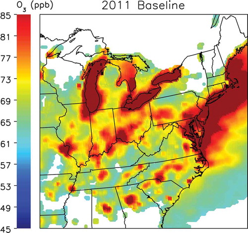
When evaluating results from an ozone-season length CMAQ run, the top 10 days containing the highest modeled daily maximum 8-hr average ozone concentrations are typically used, based on EPA modeling guidance (Wayland, 2014). However, considering only the month of July can limit the number of total days exceeding the 60 ppb threshold in a given area. For each model grid cell, we first looked for instances of at least 6, but no more than 10, days exceeding 75 ppb ozone. If six days exceeding 75 ppb were not available, the search progressed down to 74 ppb, and stepwise down until 60 ppb. For each model grid cell, the 8-hr daily maximum ozone concentration for a given scenario was determined as the maximum value found from the 3 × 3 grid surrounding a given grid cell. The spatial location of the cell contributing the maximum ozone concentration, as well as the top days found, for a given grid cell are determined in the 2011 Baseline and used in all future-year scenarios (Wayland, 2014).

Regulatory testing uses the ratio of a future-year scenario as a relative reduction factor and applies this ratio to base-year design values from monitoring stations to calculate its predicted future-year ozone concentrations and has been shown to be more accurate than using the absolute model prediction (Foley et al., 2015). However, showing concentrations only in locations with ozone monitoring stations severely limits the scope of understanding the broader impacts of the changes presented in each scenario. We wish to provide a better sense of regional change in each scenario and thus do not show reduction factors and future-year design values but rather show absolute modeled values averaged over the top 6–10 days as described above, which may add uncertainty.

Low ozone concentrations in areas that do not have 6 days where the daily maximum 8-hr average ozone concentration is above 60 ppb are represented as white regions seen in Figure 2 and subsequent figures. High ozone concentrations are seen as a result of low boundary layers over large water bodies such as the Great Lakes and Atlantic Ocean (e.g., Goldberg et al., 2014). In July 2011, most urban regions exceed the 75 ppb standard (Figure 2).

2018 Baseline

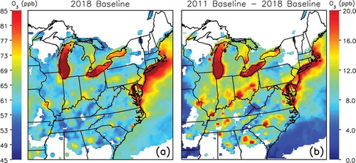
Projecting forward to the future year 2018 Baseline, surface ozone concentrations are predicted to be much lower than in 2011 (Figure 3) as a result of the decreased emissions of NO_x and VOCs across various sectors. In the 2018 Baseline run, most of the modeling domain appears to show predicted ozone concentrations below the 75 ppb. Almost 10 ppb of modeled ozone reduction is predicted in the future year across the domain, with up to 20 ppb around many city centers, although the St. Louis, MO, and Cincinnati, OH, areas and a spot in southeastern Pennsylvania near a large EGU are right at 75 ppb. Despite large improvements, many regions along the East Coast, notably along the Chesapeake Bay and Long Island, are predicted to have surface ozone concentrations exceeding 75 ppb.

Figure 3. (a) July 2018 Baseline run average 8-hr daily maximum surface ozone from the top 6–10 days of the 2011 Baseline run. Regions shown in red-orange to red exceed 75 ppb. (b) Difference plot (note different color bar) between surface ozone concentrations from the 2011 Baseline and 2018 Baseline runs.

2018 Scenario A

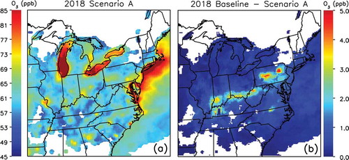
Scenario A explores the effects of all coal-fired EGUs in states considered for this study operating with their SCR or SNCR controls at historically lowest rates. By running EGUs with SCR and SNCR at the most effective observed rates, projected surface ozone in 2018 is predicted to improve by at least 2–3 ppb along the Ohio River and into Pennsylvania, with some areas improving up to 5 ppb (Figure 4b). Most regions are simulated as being below or near 75 ppb, except for the areas along the East Coast. Ozone concentrations in the areas around Cincinnati and southeastern Pennsylvania are modeled as well below 75 ppb (Figure 4a), showing benefits from the 2018 Baseline. Roughly 10% of the total U.S. population resides in the Ohio River Basin (Ohio River Valley Water Sanitation Commission [ORSANCO], 2016), so these widespread ozone reductions would benefit a substantial number of people. Areas along the western edge of the modeling domain, such as the St. Louis metropolitan area, remain unaffected in this scenario and do not change significantly in the other scenarios, because ozone concentrations can be significantly influenced by model boundary conditions.

Figure 4. (a) July 2018 Scenario A run average 8-hr daily maximum surface ozone from the top 6–10 days of the 2011 Baseline run. Regions shown in red-orange to red exceed 75 ppb. (b) Difference plot between model surface 8-hr ozone concentrations from the 2018 Baseline and 2018 Scenario A (lowest rates) runs.

2018 Scenario B

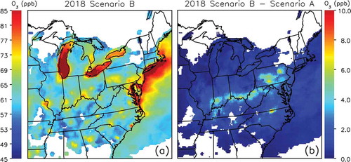
Contrary to Scenario A, EGUs were adjusted to reflect historically highest rates in Scenario B. When compared with the ideal rates of Scenario A, 4–7 ppb increases in modeled ozone are seen along the Ohio River and into Pennsylvania (Figure 5b); some city regions below 75 ppb in Scenario A are now predicted to be above 75 ppb. A few orange-colored areas reappear in Figure 5a in response to NO_x not being effectively removed from EGU sources, indicating possible risk of nonattainment. One notable area along the North Carolina and Virginia border showed an 8 ppb increase in ozone in a less populated area, where ozone concentrations approach 75 ppb. Figure 1 shows a few EGUs in the vicinity of this region, likely driving this large local increase in modeled ozone concentrations. Similarly, a small area in southwestern Indiana is close to 75 ppb in Scenario B due to its proximity to several large power plants.

Figure 5. (a) July 2018 Scenario B run average 8-hr daily maximum surface ozone from the top 6–10 days of the 2011 Baseline run. Regions shown in red-orange to red exceed 75 ppb. (b) Difference plot between surface ozone concentrations from the 2018 Scenario B (highest rates) and 2018 Scenario A (lowest rates) runs.

2018 Scenario C

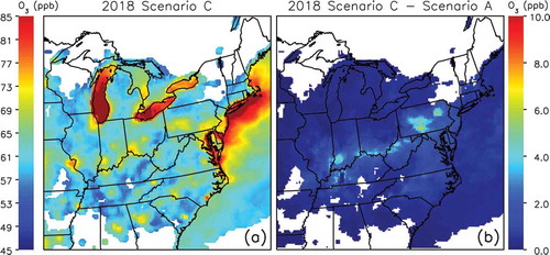
Scenario C assumed 2018 EGU emission rates matched observed NO_x rates from 2011. Although not as widespread as seen in Scenario B, Figure 6a has many of the same orange-colored areas, and only a few city regions outside the East Coast appear to show modeled ozone above 75 ppb. Similarly, the difference plot shows smaller regions with a 4–5 ppb ozone increase between lowest rates and 2011 rates (Figure 6b). Areas in Indiana and Pennsylvania near the largest power plants appear to be the most affected by NO_x increases in this scenario. EGUs operating at highest rates in Scenario B would be detrimental to meeting the 75 ppb ozone standard, but Scenario C also demonstrates a significant disadvantage if the planned, future improvements to units from 2011 fail to occur.

Figure 6. (a) July 2018 Scenario C run average 8-hr daily maximum surface ozone from the top 6–10 days of the 2011 Baseline run. Regions shown in red-orange to red exceed 75 ppb. (b) Difference plot between surface ozone concentrations from the 2011 Scenario C (2011 rates) and 2018 Scenario A (lowest rates) runs.

2018 Scenario D

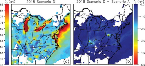
In Scenario D, we targeted the coal-fired power plants that are not anticipated to shut down or install SCR technology by 2018. In addition to the benefits gained from running installed controls at historically lowest rates, NO_x emissions from these uncontrolled units were reduced to reflect benefits of full SCR adoption in the states considered for this study. “Uncontrolled” refers only to the lack of postcombustion controls, as these units may utilize less efficient combustion controls such as low-NO_x burners or overfire air (EPA, 2015e, 2015f). Figure 7a shows all areas along the Ohio River and into Pennsylvania below 75 ppb in this scenario, and only a couple of urban regions outside the East Coast cities appear to still show modeled ozone concentrations greater than 75 ppb. Two regions in particular seem to gain the most significant benefits from this additional reduction strategy. One area is along the Ohio River separating the states of Indiana and Kentucky, where ozone is predicted to decrease an additional 2–3 ppb, and another is around the shared Maryland, Pennsylvania, and West Virginia borders, where ozone is predicted to decrease an additional 3–4 ppb (Figure 7b).

Figure 7. (a) July 2018 Scenario D run average 8-hr daily maximum surface ozone from the top 6–10 days of the 2011 Baseline run. Regions shown in red-orange to red exceed 75 ppb. (b) Difference plot between surface ozone concentrations from the 2018 Scenario D (lowest rates with additional SCR) and 2018 Scenario A (lowest rates) runs.

Improvements to Mid-Atlantic East Coast

Results for Scenario A demonstrated large, noticeable modeled ozone improvements to areas along the Ohio River and into Pennsylvania when EGUs are operated at lowest rates when compared with the 2018 Baseline, but there are also important improvements to coastal states in the Mid-Atlantic region, where ozone concentrations can be high (Figure 8a). In addition to the larger, more obvious benefits in Pennsylvania, 1.5–2 ppb of predicted reduction is seen in much of the state. A majority of Maryland and Delaware is predicted to see about a 1.5 ppb ozone reduction from Scenario A, as do parts of Virginia.

Figure 8. Ozone difference plots demonstrating modeled reductions from the 2018 Baseline in the coastal Mid-Atlantic states from (a) Scenario A (lowest rates) and (b) Scenario D (lowest rates with additional SCR).

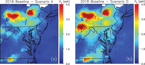
In the simulation where currently uncontrolled units now include SCRs, Scenario D, much of the Mid-Atlantic coast realizes a 1.5–2 ppb of modeled ozone reduction from the 2018 Baseline, with some downwind regions closer to affected units reaching widespread modeled reductions of 2.5–3 ppb (Figure 8b). This scenario also now brings a predicted reduction of up to 1.5 ppb to much of New Jersey as well. Although the quantity of total modeled ozone benefit along the coast from these scenarios may not seem very significant given the much larger reductions found in other upwind areas, an overall 2 ppb reduction could be monumental for areas that have been on the edge of meeting attainment.

New ozone standard—70 ppb

Regions that have already struggled with meeting a 75 ppb standard will undoubtedly require further regulations to attain the new 70 ppb standard. Areas that have historically or recently been in attainment of the NAAQS may require further emission restrictions to attain the new standard. This study may provide valuable insight into the efficacy of EGU control strategies and a model framework to test ways for attaining the new standard.

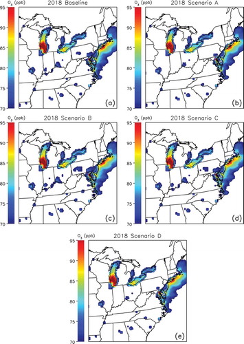
The modeling results in Figure 9 show only model grid cells where average 8-hr ozone is predicted to be 70 ppb or greater. Figure 9a suggests that several regions could exceed a 70 ppb standard in 2018 with expected controls in place (future case baseline), but many regions could demonstrate attainment if EGU controls are operated at their historically lowest rates (Figure 9b). Ozone decreased in Scenario A, bringing modeled ozone in all of Indiana and Kentucky below 70 ppb. The area east of Pittsburgh with modeled ozone previously over 70 ppb completely disappears, and the area west of Philadelphia decreases in size significantly. However, if EGUs operate at their highest rates (Figure 9c), most regions along the Ohio River and throughout Pennsylvania have modeled ozone exceeding 70 ppb, and although not as extreme, 2011 rates could also leave these regions with ozone concentrations above 70 ppb (Figure 9d). Adding SCRs to uncontrolled units, in addition to running other EGUs at lowest rates, further decreases the size of the areas around Cincinnati and west of Philadelphia with predicted ozone concentrations greater than 70 ppb (Figure 9e). Scenarios A and D marginally decrease the size of the widespread area exceeding 70 ppb over the East Coast, decreasing modeled ozone below 70 ppb most in the inland/westernmost grid cells of Maryland and Virginia.

Figure 9. July average daily 8-hr maximum surface ozone from the top 6–10 days of 2011 Baseline for (a) 2018 Baseline, (b) Scenario A (lowest rates), (c) Scenario B (highest rates), (d) Scenario C (2011 rates), and (e) Scenario D (lowest rates with additional SCR). Areas where modeled ozone exceeds the 70 ppb NAAQS are plotted, whereas areas below the new standard are in white.

Discussion

Model results show beneficial ozone reductions in coastal Mid-Atlantic States from running existing SCR and SNCR at optimal rates on upwind EGUs. Although these cost-effective reductions prove beneficial to citizens of areas along the coast, the greatest modeled benefits are seen nearby where the largest EGUs are located (Figure 4b). For many areas along the Ohio River and through Pennsylvania, the difference between EGUs running their controls and not running controls can often result in an improvement of 5 ppb modeled ozone or greater (Table 4). Notably, 5 ppb is the difference between the 2008 and 2015 ozone standards, suggesting optimal use of EGU controls could play a critical and beneficial role in making the difference needed for attainment of the 2015 ozone standard in the coming years.

Table 4. Summary of surface ozone changes for affected areas in each modeling scenario.

Scenario	EGU NOx rates	Average surface ozone change	Maximum change
2018 Scenario A	Historically lowest	2–3 ppb decrease from 2018 Baseline	5 ppb decrease in several locations
2018 Scenario B	Historically highest	4–7 ppb increase from Scenario A	8 ppb increase at NC/VA border
2018 Scenario C	Same as 2011	4–5 ppb increase from Scenario A	7 ppb increase in south-central PA
2018 Scenario D	Historically lowest + SCR on uncontrolled units	2–3 ppb decrease from Scenario A	4 ppb decrease at MD/PA/WV borders

Scenario A provides the most achievable approach, as no additional capital investment is required. This scenario represented coal-fired units operating with their lowest average ozone season NO_x emission rates, which accounts for a certain level of variability (start-ups, shut-downs, variable loads, cycling the SCR/SNCR system off, etc.) throughout the ozone season, and not the absolute lowest rates that would constrain the unit with an emission factor that may not be sustainable over the long term. In the 2015 ozone season, CAMD data revealed that roughly a third of units were found to have average ozone season emission rates that achieved rates even lower than what was used from the time frame in this study. Units that did not achieve the lowest rates did not fail to do so because these low rates were unattainable, but because regulatory and market mechanisms were used to comply. Cap-and-trade policies were implemented with the general idea to incentivize utilization of SCR/SNCR while also allowing for flexibility. Over time, the market has evolved to a point where it can sometimes be cheaper to purchase allowances than to run existing controls (OTC, 2015). In order to achieve meaningful NO_x reductions that would allow areas to achieve attainment of the ozone NAAQS, the market system would need to be adjusted, as current regulatory limits and costs of allowances appear too lenient to require widespread, optimal use of SCR/SNCR systems.

Operating EGUs at optimal rates will provide important benefits, but our modeling predicts that overall, much of the East Coast may require additional pollutant reductions from other emission sources to attain the new 70 ppb standard. Although NO_x emissions from on-road and nonroad sources will decrease from 2011 to 2018, they are expected to still constitute over a third of total NO_x emissions (Table 3) and, in addition to EGUs, could be another two possible source groups targeted for significant NO_x reductions. Other point sources not belonging to the EGU or oil and gas sectors make up almost 20% of remaining NO_x emissions expected in 2018. Moving forward, NO_x reductions from sources in this category, such as cement kilns, industrial/commercial/institutional (ICI) boilers, and other industrial and manufacturing facilities may be required to drive down total NO_x emissions (Table 3).

Evaluations of the 2011 U.S. emissions inventories suggest that estimates of NO_x emissions from vehicular sources are overestimated by roughly a factor of 2 (Anderson et al., 2014, Travis et al., 2016), and that the recycling of NO₂ is underestimated in CB05 (Canty et al., 2015); although revision 2 of version 6 of the Chemical Bond mechanism (CB6r2) appears to simulate NO_x chemistry more accurately (Goldberg et al., 2016). As a result, emissions of NO_x from EGUs would be expected to have an even broader range of influence and greater impact on ozone compared with on-road sources. Thus, the results presented here could be viewed as conservative and may represent a lower limit for significant ozone reductions achieved from running SCR and SNCR controls on EGUs at optimal rates.

Conclusion

Numerical simulations indicate that the substantial investment in SCR and SNCR units on power plants in the eastern U.S. has provided an appreciable beneficial impact on air quality. Current regulations allow these units to be turned off for considerable periods as long as annual and ozone season emissions caps are met. However, our model results indicate that the difference between the recorded least-effective NO_x removal rates and the rates from complete adoption and optimal utilization of NO_x removal systems on coal-fired power plants produces a calculated change in ozone that approaches 10 ppb. Even without new capital investment, predicted concentrations of ozone in 2018 could be improved by up to 5 ppb solely by running existing, operable technology at optimal rates.

Acknowledgment

The authors would like to thank the U.S. Environmental Protection Agency for providing surface SMOKE and MCIP output files and New York State Department of Environmental Conservation for assistance with CMAQ configurations and benchmarking. The authors would also like to thank Hannah Ashenafi for her assistance in analyzing 2015 ozone season CAMD data.

Funding

This study was supported by the Maryland Department of the Environment under the Regional Atmospheric Measurement Modeling and Prediction Program (RAMMPP) program.

Supplementary Material

Supplemental data for this article can be accessed on the publisher’s website.

Additional information

Funding

This study was supported by the Maryland Department of the Environment under the Regional Atmospheric Measurement Modeling and Prediction Program (RAMMPP) program.

Notes on contributors

Timothy Vinciguerra

Timothy Vinciguerra is a graduate student in the Department of Chemical and Biomolecular Engineering, University of Maryland, College Park.

Emily Bull

Emily Bull is the Natural Resources Planner for the Maryland Department of the Environment.

Timothy Canty

Timothy Canty, Ph.D., is a research assistant professor and director of undergraduate and Masters of Professional Studies: Atmospheric and Oceanic Science programs with the Department of Atmospheric and Oceanic Sciences, University of Maryland, College Park.

Hao He

Hao He, Ph.D., is a research associate with the Department of Atmospheric and Oceanic Sciences, University of Maryland, College Park.

Eric Zalewsky

Eric Zalewsky is a research scientist with the New York State Department of Environmental Conservation.

Michael Woodman

Michael Woodman is chief of the Air Quality, Measurements, Modeling, and Analysis Division, Maryland Department of the Environment.

George Aburn

George Aburn is the director for the Air & Radiation Management Administration, Maryland Department of the Environment.

Sheryl Ehrman

Sheryl Ehrman, Ph.D., is Keystone Professor and Chair of the Department of Chemical and Biomolecular Engineering, University of Maryland, College Park.

Russell R. Dickerson

Russell R. Dickerson, Ph.D., is a professor with the Department of Atmospheric and Oceanic Sciences, University of Maryland, College Park.

References

- Anderson, D.C., C.P. Loughner, G. Diskin, A. Weinheimer, T.P. Canty, R.J. Salawitch, H.M. Worden, A. Fried, T. Mikoviny, A. Wisthaler, and R.R. Dickerson. 2014. Measured and modeled CO and NOy in DISCOVER-AQ: An evaluation of emissions and chemistry over the eastern US. Atmos. Environ. 96:78–87. doi: 10.1016/j.atmosenv.2014.07.004.
- Appel, K.W., G.A. Pouliot, H. Simon, G. Sarwar, H.O.T. Pye, S.L., Napelenok, F. Akhtar, and S.J. Roselle. 2013. Evaluation of dust and trace metal estimates from the Community Multiscale Air Quality (CMAQ) model version 5.0. Geosci. Model Dev. 6:883–899. doi: 10.5194/gmd-6-883-2013.
- Bey, I., D.J. Jacob, R.M. Yantosca, J.A. Logan, B.D. Field, A.M. Fiore, Q.B. Li, H.G.Y. Liu, L.J. Mickley, and M.G. Schultz. 2001. Global modeling of tropospheric chemistry with assimilated meteorology: Model description and evaluation. J. Geophys. Res. 106(D19):23073–23095. doi: 10.1029/2001JD000807.
- Canty, T.P., L. Hembeck, T.P. Vinciguerra, D.C. Anderson, D.L. Goldberg, S.F., Carpenter, D.J. Allen, C.P. Loughner, R.J. Salawitch, and R.R. Dickerson. 2015. Ozone and NOx chemistry in the eastern US: Evaluation of CMAQ/CB05 with satellite (OMI) data. Atmos. Chem. Phys. 15:10965–10982. doi: 10.5194/acp-15-10965-2015.
- CMAQ. 2015. CMAQ version 5.0.2 (April 2014 release) Technical Documentation. http://www.airqualitymodeling.org/cmaqwiki/index.php?title=CMAQ_version_5.0.2_%28April_2014_release%29_Technical_Documentation (accessed December 11, 2015).
- Crawford, J.H., R.R. Dickerson, and J. Hains. 2014. DISCOVER-AQ observations and early results. Environ. Manage. 9:8–15.
- Crutzen, PJ. 1974. Photochemical reactions initiated by and influencing ozone in unpolluted tropospheric air. Tellus 26:47–57. doi: 10.1111/tus.1974.26.issue-1-2
- Dolwick, P., D. Kang, K. Baker, S. Phillips, N. Possiel, H. Simon, J. Kelly, C. Misenis, and B. Timin. 2014. Initial evaluation of 2011 CMAQ and CAMx simulations during the DISCOVER-AQ period in the Mid-Atlantic. Presented at the 13th Annual Community Modeling and Analysis System (CMAS) Conference, Chapel Hill, NC, October 27–29. https://www.cmascenter.org/conference/2014/slides/pat_dolwick_three-dimensional_evaluation_2014.pptx (accessed December 16, 2015).
- Duncan, B.N., Y. Yoshida, J.R. Olsen, S. Sillman, R.V. Martin, L. Lamsal, Y. Hu, K.E. Pickering, D.J. Allen, C. Retscher, and J.H. Crawford. 2010. Application of OMI observations to a space-based indicator of NOx and VOC controls on surface ozone formation. Atmos. Environ. 44:2213–2223. doi: 10.1016/j.atmosenv.2010.03.010.
- Foley, K.M., P. Dolwick, C. Hogrefe, H. Simon, B. Timin, and N. Possiel. 2015. Dynamic evaluation of CMAQ part II: Evaluation of relative response factor metrics for ozone attainment demonstrations. Atmos. Environ. 103:188–195. doi: 10.1016/j.atmosenv.2014.12.039
- Foley, K.M., S.J. Roselle, K.W. Appel, P.V. Bhave, J.E. Pleim, T.L. Otte, R. Mathur, G. Sarwar, J.O. Young, R.C. Gilliam, C.G. Nolte, J.T. Kelly, A.B. Gilliland, and J.O. Bash. 2010. Incremental testing of the Community Multiscale Air Quality (CMAQ) modeling system version 4.7. Geosci. Model. Dev. 3:205–226. doi: 10.5194/gmd-3-205-2010
- Goldberg, D.L., C.P. Loughner, M. Tzortziou, J.W. Stehr, K.E. Pickering, L.T. Marufu, and R.R. Dickerson. 2014. Higher surface ozone concentrations over the Chesapeake Bay than over the adjacent land: Observations and models from the DISCOVER-AQ and CBODAQ campaigns. Atmos. Environ. 84:9–19. doi: 10.1016/j.atmosenv.2013.11.00.
- Goldberg, D.L., T.P. Vinciguerra, D.C. Anderson, L. Hembeck, T.P. Canty, S.H. Ehrman, D.K. Martins, R.M. Stauffer, A.M. Thompson, R.J. Salawitch, and R.R. Dickerson. 2016. CAMx ozone source attribution in the eastern United States using guidance from observations during DISCOVER-AQ Maryland. Geophys. Res. Lett. 43:2249–2258. doi: 10.1002/2015GL067332.
- Haagensmit, A.J., C.E. Bradley, and M.M. Fox. 1953. Ozone formation in photochemical oxidation of organic substances. Ind. Eng. Chem. 45:2086–2089. doi: 10.1021/ie50525a044
- Hains, J.C., B.F. Taubman, A.M. Thompson, J.W. Stehr, L.T. Marufu, B. Doddridge, and R.R. Dickerson. 2008. Origins of chemical pollution derived from Mid-Atlantic aircraft profiles using a clustering technique. Atmos. Environ. 42:1727–1741. doi: 10.1016/j.atmosenv.2007.11.052.
- He, H., L. Hembeck, K.M. Hosley, T.P. Canty, R.J. Salawitch, and R.R. Dickerson. 2013a. High ozone concentrations on hot days: The role of electric power demand and NOx emissions. Geophys. Res. Lett. 40:5291–5294. doi: 10.1002/grl.50967.
- He, H., C.P. Loughner, J.W. Stehr, H.L. Arkinson, L.C. Brent, M.B. Follette-Cook, M.A. Tzortziou, K.E. Pickering, A.M. Thompson, D.K. Martins, G.S. Diskin, B.E. Anderson, J.H. Crawford, A.J. Weinheimer, P. Lee, J.C. Hains, and R.R. Dickerson. 2014. An elevated reservoir of air pollutants over the Mid-Atlantic States during the 2011 DISCOVER-AQ campaign: Airborne measurements and numerical simulations. Atmos. Environ. 85:18–30. doi: 10.1016/j.atmosenv.2013.11.039.
- He, H., J.W. Stehr, J.C. Hains, D.J. Krask, B.G. Doddridge, K.Y. Vinnikov, T.P. Canty, K.M. Hosley, R.J. Salawitch, H.M. Worden, and R.R. Dickerson. 2013b. Trends in emissions and concentrations of air pollutants in the lower troposphere in the Baltimore/Washington airshed from 1997 to 2011. Atmos. Chem. Phys. 13:7859–7874. doi: 10.5194/acp-13-7859-2013.
- Karamchandani, P., J. Johnson, G. Yarwood, and E. Knipping. 2014. Implementation and application of sub-grid-scale plume treatment in the latest version of EPA’s third-generation air quality model, CMAQ 5.01. J. Air Waste Manage. Assoc. 64:453–467. doi: 10.1080/10962247.2013.855152.
- McNevin, T.F. 2016. Recent increases in nitrogen oxide (NOx) emissions from coal-fired electric generating units equipped with selective catalytic reduction. J. Air Waste Manage. Assoc. 66:66–75. doi:10.1080/10962247.2015.1112317.
- Nolte, C.G., K.W. Appel, J.T. Kelly, P.V. Bhave, K.M. Fahey, J.L. Collett Jr., L. Zhang, and J.O. Young. 2015. Evaluation of the Community Multiscale Air Quality (CMAQ) model v5.0 against size-resolved measurements of inorganic particle composition across sites in North America. Geosci. Model Dev. 8:2877–2892. doi: 10.5194/gmd-8-2877-2015.
- Ohio River Valley Water Sanitation Commission. River Facts/Conditions. http://www.orsanco.org/factcondition (accessed January 15, 2016).
- Ozone Transport Commission. 2015. Comparison of CSAPR Allowance Prices to Cost of Operating SCR Controls. Final Draft. OTC Stationary and Area Source Committee, Largest Contributors Workgroup. http://www.otcair.org/upload/Documents/Reports/Draft%20Final%20Allowance%20v%20SCR%20operating%20costs%2004-15-15.pdf (accessed June 15, 2016).
- Roy, A., and Y. Choi. 2015. New Directions: Potential impact of changing the coal-natural gas split in power plants: An emissions inventory perspective for criteria pollutants. Atmos. Environ. 102:413–415. doi: 10.1016/j.atmosenv.2014.10.063.
- Ryan, W.F., B.G. Doddridge, R.R. Dickerson, R.M. Morales, K.A. Hallock, P.T. Roberts, D.L. Blumenthal, J.A. Anderson, and K.L. Civerolo. 1998. Pollutant transport during a regional O3 episode in the Mid-Atlantic States. J. Air Waste Manage. Assoc. 48:786–797. doi: 10.1080/10473289.1998.10463737
- Sarwar, G., H. Simon, P. Bhave, and G. Yarwood. 2012. Examining the impact of heterogeneous nitryl chloride production on air quality across the United States. Atmos. Chem. Phys. 12:6455–6473. doi: 10.5194/acp-12-6455-2012.
- Smith, J.B., and D. Tirpak. 1989. The Potential Effects of Global Climate Change on the United States. EPA-230-05-89-050. Washington, DC: U.S. Environmental Protection Agency.
- SMOKE. 2012. SMOKE v3.1 User’s Manual. The Institute for the Environment, The University of North Carolina at Chapel Hill. https://www.cmascenter.org/smoke/documentation/3.1/manual_smokev31.pdf (accessed December 11, 2015).
- Taubman, B.F., J.C. Hains, A.M. Thompson, L.T. Marufu, B.G. Doddridge, J.W. Stehr, C.A. Piety and R.R. Dickerson. 2006. Aircraft vertical profiles of trace gas and aerosol pollution over the Mid-Atlantic United States: Statistics and meteorological cluster analysis. J. Geophys. Res. Atmos. 111(D10):D10S07. doi: 10.1029/2005JD006196.
- Taubman, B.F., L.T. Marufu, C.A. Piety, B.G. Doddridge, J.W. Stehr, and R.R. Dickerson. 2004. Airborne characterization of the chemical, optical, and meteorological properties, and origins of a combined ozone/haze episode over the eastern U.S. J. Atmos. Sci. 61:1781–1793. doi: 10.1175/1520-0469(2004)061<1781:ACOTCO>2.0.CO;2
- Travis, K.R., D.J. Jacob, J.A. Fisher, P.S. Kim, E.A. Marais, L. Zhu, K. Yu, C.C. Miller, R.M. Yantosca, M.P. Sulprizio, et al. 2016. NOx emissions, isoprene oxidation pathways, vertical mixing, and implications for surface ozone in the Southeast United States. Atmos. Chem. Phys. Discuss. doi: 10.5194/acp-2016-110.
- U.S. Energy Information Administration. 2016. Monthly Energy Review January 2016. DOE/EIA-0035(2016/1). http://www.eia.gov/totalenergy/data/monthly/pdf/mer.pdf (accessed February 18, 2016).
- U.S. Environmental Protection Agency. 2003a. Air Pollution Control Technology Fact Sheet, Selective Catalytic Reduction (SCR). EPA-452/F-03-032. http://www3.epa.gov/ttn/catc/dir1/fscr.pdf (accessed December 8, 2015).
- U.S. Environmental Protection Agency. 2003b. Air Pollution Control Technology Fact Sheet, Selective Non-Catalytic Reduction (SNCR). EPA-452/F-03-031. http://www3.epa.gov/ttn/catc/dir1/fsncr.pdf (accessed December 8, 2015).
- U.S. Environmental Protection Agency. 2008. National Ambient Air Quality Standards for ozone; final rule. Fed. Regist. 73:16436–16514.
- U.S. Environmental Protection Agency. 2014a. Technical Support Document (TSD), Preparation of Emissions Inventories for the Version 6.0, 2011 Emissions Modeling Platform. http://www3.epa.gov/ttn/chief/emch/2011v6/outreach/2011v6_2018base_EmisMod_TSD_26feb2014.pdf (accessed December 16, 2015).
- U.S. Environmental Protection Agency. 2014b. Meteorological Model Performance for Annual 2011 WRF v3.4 Simulation. https://www3.epa.gov/scram001/reports/MET_TSD_2011_final_11-26-14.pdf (accessed March 24, 2016).
- U.S. Environmental Protection Agency. 2014c. 2011ed_v6_11f_state_sector_totals. ftp://ftp.epa.gov/EmisInventory/2011v6/v1platform/reports/2011_emissions/2011ed_v6_11f_state_sector_totals.xlsx (accessed December 16, 2015).
- U.S. Environmental Protection Agency. 2014d. Technical Support Document (TSD), Preparation of Emissions Inventories for the Version 6.1, 2011 Emissions Modeling Platform. http://www3.epa.gov/ttn/chief/emch/2011v6/2011v6.1_2018_2025_base_EmisMod_TSD_nov2014_v6.pdf (accessed December 16, 2015).
- U.S. Environmental Protection Agency. 2015a. SIP Status and Information. http://www3.epa.gov/airquality/urbanair/sipstatus/ (accessed December 16, 2015).
- U.S. Environmental Protection Agency. 2015b. National Ambient Air Quality Standards for ozone; final rule. Fed. Regist. 80:65292–65468.
- U.S. Environmental Protection Agency. 2015c. Cross-State Air Pollution Rule (CSAPR). http://www3.epa.gov/crossstaterule/(accessed December 8, 2015).
- U.S. Environmental Protection Agency. 2015d. Emissions Monitoring, Clean Air Markets. http://www2.epa.gov/airmarkets/emissions-monitoring (accessed December 16, 2015).
- U.S. Environmental Protection Agency. 2015e. Technical Support Document (TSD) for the Cross-State Air Pollution Rule for the 2008 Ozone NAA. EPA-HQ-OAR-2015-0500. http://www.epa.gov/sites/production/files/2015-11/documents/egu_nox_mitigation_strategies_tsd_0.pdf ( accessed February 18, 2016).
- U.S. Environmental Protection Agency. 2015f. EPA Base Case v.5.14 Using IPM Incremental Documentation. http://www.epa.gov/sites/production/files/2015-08/documents/epa_base_case_v514_incremental_documentation.pdf (accessed February 18, 2016).
- U.S. Environmental Protection Agency. 2016. Cross-State Air Pollution Rule (CSAPR): Frequently Asked Questions. http://www3.epa.gov/crossstaterule/faqs.html (accessed March 1, 2016).
- Wayland, R. 2014. Draft Modeling Guidance for Demonstrating Attainment of Air Quality Goals for Ozone, PM2.5, and Regional Haze. Memorandum. http://www3.epa.gov/scram001/guidance/guide/Draft_O3-PM-RH_Modeling_Guidance-2014.pdf (accessed December 16, 2015).