Near-roadway monitoring of vehicle emissions as a function of mode of operation for light-duty vehicles

ABSTRACT

Determination of the effect of vehicle emissions on air quality near roadways is important because vehicles are a major source of air pollution. A near-roadway monitoring program was undertaken in Chicago between August 4 and October 30, 2014, to measure ultrafine particles, carbon dioxide, carbon monoxide, traffic volume and speed, and wind direction and speed. The objective of this study was to develop a method to relate short-term changes in traffic mode of operation to air quality near roadways using data averaged over 5-min intervals to provide a better understanding of the processes controlling air pollution concentrations near roadways. Three different types of data analysis are provided to demonstrate the type of results that can be obtained from a near-roadway sampling program based on 5-min measurements: (1) development of vehicle emission factors (EFs) for ultrafine particles as a function of vehicle mode of operation, (2) comparison of measured and modeled CO₂ concentrations, and (3) application of dispersion models to determine concentrations near roadways. EFs for ultrafine particles are developed that are a function of traffic volume and mode of operation (free flow and congestion) for light-duty vehicles (LDVs) under real-world conditions. Two air quality models—CALINE4 (California Line Source Dispersion Model, version 4) and AERMOD (American Meteorological Society/U.S. Environmental Protection Agency Regulatory Model)—are used to predict the ultrafine particulate concentrations near roadways for comparison with measured concentrations. When using CALINE4 to predict air quality levels in the mixing cell, changes in surface roughness and stability class have no effect on the predicted concentrations. However, when using AERMOD to predict air quality in the mixing cell, changes in surface roughness have a significant impact on the predicted concentrations.

Implications: The paper provides emission factors (EFs) that are a function of traffic volume and mode of operation (free flow and congestion) for LDVs under real-world conditions. The good agreement between monitoring and modeling results indicates that high-resolution, simultaneous measurements of air quality and meteorological and traffic conditions can be used to determine real-world, fleet-wide vehicle EFs as a function of vehicle mode of operation under actual driving conditions.

Introduction

The U.S. Environmental Protection Agency (EPA) has established a near-road ambient monitoring program that stems from concerns for the health of populations exposed to traffic-related emissions of particles and gases. The monitoring program encourages the use of monitoring methods that supply a greater time resolution for comparison with air quality standards (Venkatram et al., 2007; Fruin et al., 2008; National Ambient Air Quality Standards [NAAQS], 2015). Determination of the effect of vehicle emissions on air quality near roadways is important because vehicles are a major source of air pollution. A comprehensive monitoring program near roadways that can determine the impact of vehicle emissions on air quality requires not only air quality measurements near roadways but also includes (1) determination of the number of vehicles on the roadway and their speed and mode of operation (congestion or free flow), (2) meteorological conditions (wind speed and direction and atmospheric stability conditions) that impact the dilution of emissions, and (3) the application of vehicle emission and dispersion models. Because changes in air quality near roadways is very episodic due to rapid changes in traffic patterns, monitoring programs need to measure in time periods as short as 5 minutes. Combining model-calculated vehicle emission factors and dilution of tail-pipe emissions with short-term measurements of air quality near roadways allows determination of vehicle emission impacts under varying real-world conditions.

Numerous investigators have measured air quality near roadways and applied models to quantify processes related to changes in traffic conditions (Zhu et al., 2002a, 2002b, 2005; Morawska et al., 2008). They have identified that changes in air quality near roadways are related to (1) the rate of emissions from vehicle as a function of vehicle mode of operation (congestion or free flow), (2) the number of vehicles, (3) the rate of dilution due to traffic flow and atmospheric turbulence, and (4) the distance from the roadway. Prior efforts to relate air quality levels near roadways to these parameters has been impeded by the inability to relate short-term changes in traffic flow (minutes) to long-term measurements of air quality (hours) and do not fully reveal the dynamics of the process. Emission factors (EFs) that account for vehicle operating mode are needed for modeling vehicle emissions at lower speeds and under congested conditions and for the establishment of ambient and vehicle emission standards. This study measures air quality levels in 5-min intervals that can be related to short-term changes in vehicle mode of operation and level of service. Combining short-term air pollution measurements with model predictions of dilution of emissions allows estimates of emission factors as a function of vehicle mode of operation and traffic conditions. Emission factors are determined for the actual vehicle fleet under varying real-world conditions. However, the simultaneous measurement of air quality concentrations, meteorological conditions, and traffic patterns produces data with a high degree of uncertainty; therefore, the development of emission factors for free flow and congestion conditions is generated from data with a high error factor (Kumar et al., 2010).

The available data on emissions near highways generally include measurements of emissions from both light-duty vehicles (LDVs) and heavy-duty vehicles (HDVs). For example, diesel vehicles are typically under 5% of the total vehicles on roadways but contribute more than half of the ultrafine particles (UFPs) (Kirchstetter et al., 1999; Zhu et al., 2005), and it is difficult to accurately determine the contribution due only to gasoline-powered vehicles. Therefore, this study was conducted near a roadway that was restricted to LDVs and focused on petrol-fueled LDVs.

The objective of this study is to develop a method to relate short-term changes in traffic mode of operation to air quality near roadways using data averaged over 5-min intervals to provide a more comprehensive understanding of the processes controlling air pollution concentrations near highways and also to provide the opportunity to verify dispersion models that characterize the dilution and transport of pollutants near roadways over short time periods. This paper provides EFs that are a function of traffic volume and mode of operation (free flow and congestion) for LDVs under real-world conditions. Congestion represents hindered, unstable vehicle flow conditions.

Materials and methods

A near-roadway monitoring program was undertaken in Chicago, Illinois, between August 4 and October 30, 2014, to measure ultrafine particles, carbon dioxide (CO₂), carbon monoxide (CO), traffic volume and speed, and wind direction and speed. Figure 1 is a map of the sampling site, in which the sampling locations and the surrounding area are presented. Samples were collected at 5-min intervals for 11 sampling days in the afternoon and evening from 3:00 p.m. to 8:00 p.m. for time periods of 2–5 hr depending on traffic and meteorological conditions. Measurements were made at the edge of the roadway (site A: 3 m west and site B: 3 m east) and at downwind distances of 30, 60, 90, 150, and 200 m sequentially and 100 m upwind from the edge of the highway as background. Background samples were collected at the beginning and the end of each sampling day; 5-min wind speed and traffic were measured simultaneously with background samples. At each sampling location, concentrations of CO, CO₂, and UFPs were measured simultaneously with meteorological conditions, including wind speed and direction, temperature, and relative humidity. Traffic volume and speed were obtained from video recordings taken simultaneously with the other measurements for a 135-m-long road segment (Figure 1). There were no other traffic sensors used in this study. Total particle number concentration with size 0.02–1 μm was measured at 1 m above the ground by a condensation particle counter (CPC) (TSI 8525; TSI, 2015). Daily zero check of the CPC was performed. CO (0-200ppm) and CO₂ concentrations (0–200 ppm) was measured by a hand-held gas sampler (AQ PRO 3; E Instruments, 2015). Both instruments were calibrated in July 2014 before the sampling program started. CPC measurements were periodically compared with two other CPCs (TSI 3007; Technical Support, Inc, 2002) and a Scanning Mobility Particle Sizer Spectrometer (SMPS; TSI Incorporated, Shoreview, MN). Wind speed and direction and temperature were measured and logged with a hand-held weather station (Kestrel 4500; Kestrelmeters, Minneapolis, MN). A video recorder (Sony HDR-CX330; Sony Corporation of America, New York, NY) was used to record traffic information, including traffic volume and speed, with 2-min samples taken for each 5-min time period. Each 5 min was a separate sampling period; 5-min averages were used to record and reflect the short-term variation in traffic flow. Wind speed ranged from 0.5 to 3 km/hr and was from the east during nine sampling days so that sampling was conducted on the west side of the roadway.

Figure 1. Map of sampling site near Lake Shore Drive with the north- and southbound lanes and sampling locations identified.

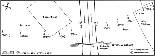
Selection of an appropriate sampling site is important in order to allow the results to be universally applicable and not dependent on features associated with local conditions. Lake Shore Drive is a limited-access roadway with eight lanes and north/southbound traffic directions. This site is ideal for this study for a number of reasons. The roadway is level with no grade, restricted to LDVs only, and without highway barriers and separation to restrict airflow. The site has varying traffic flow conditions. The surrounding terrain is level in both the east and west directions, and there are no other major highways or emission sources and no obstacles present for at least 350 m. A pedestrian walkway is located above the center of the roadway at the site where video recording of traffic from all lanes is possible.

Method for determination of traffic emission factors

Traffic emission factors were determined using ensemble means of air quality measurements. The ensemble mean is the arithmetic average of a variable obtained from repeating an experiment many times under the same general conditions. The calculation of a dilution factor (DL) is required that describes the dilution due to roadway mixing and atmospheric dispersion of tail pipe emissions. The DL is determined from CALINE4 (California Line Source Dispersion Model, version 4) based on measured meteorological and traffic flow conditions. DLs are also calculated with CO emission factors determined from MOVES 2014 (Motor Vehicle Emissions Simulator; EPA, 2014) and measured CO concentrations using eq 1 based on the assumption that DL are the same for CO and UFPs. The results indicate that the ensemble mean dilutions were similar, with an average of 2.2 × 10¹² cm³ for congestion or free flow for both models.

When simultaneous measurements of meteorological conditions, traffic flow, and atmospheric concentrations of UFPs are available, it is possible to determine emission factors from vehicles as follows:

(1)

where EF is the vehicle emission factor, C is measured ambient concentration, DL is a model (CALINE4)-calculated dilution factor that describes the dilution due to roadway mixing and atmospheric dispersion of tail pipe emissions, N is number of vehicles, and C_b is background concentration. The equation can be applied to a particular 5-min sample and also to ensemble means. Categorizing the data by traffic flow rate (N) allows the determination of the vehicle emission factor as a function of traffic speed, traffic volume, and level of service on the roadway (congestion and free flow).

Determination of free flow and congestion EFs

Since we have measurements of the free flow and congestion traffic volumes (traffic mix), we are able to evaluate the EFs for free flow and congestion using eq 2:

(2)

EF_fleet, EF_FF, and EF_C are the emission rates for the fleet, free flow, and congestion vehicles and N_fleet, N_FF, and N_C are the total traffic flow for each condition (vehicle/km). Zhang and Wexler (2004) used similar approach to evaluate the EFs for a mix of trucks and nontrucks (Zhang et al., 2005). When there is no congestion, the (EF_FF × N_FF) are equal to the measured (EF_fleet × N_fleet). When there is a mix of free flow and congestion traffic conditions, we can subtract the free flow conditions from the fleet conditions to determine the congestion EFs.

Results

Characterization of near-roadway measurements

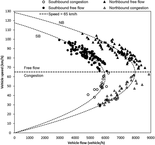
Figure 2 provides information on the speed-flow relationship during the sampling program. The speed-flow relationship is typical of traffic conditions on roadways (Mannering et al., 2013). The figure shows that vehicle flow is at maximum capacity with the corresponding speed near 65 km/hr and decreases for higher and lower speeds. The traffic speed of 65 km/hr separates traffic into free flow and congestion conditions. The traffic is considered free flow on the upper part of the speed-flow curve with speed above 65 km/hr; when the speed is below 65 km/hr, traffic is hindered and in a highly congested and unstable condition (Mannering et al., 2013). Free flow represents conditions when the traffic flow is unhindered by other vehicles. The traffic patterns were different for the north- and southbound lanes due to different traffic conditions. There were no time periods when both directions were congested. The figure indicates that there was significant variation in traffic conditions that can be related to vehicle EFs.

Figure 2. Relationship between measured traffic vehicle flow and speed for north- and southbound lanes separated into free flow (speed >65 km/hr) and congestion (speed <65 km/hr).

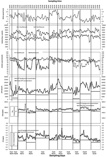
Figure 3 provides information on near-roadway measurements. There were a total of 225 measurements made during the afternoon and evening time on 11 different days. Temperatures varied between 50 and 90 °F. Wind speed ranged from 0.14 to 0.83 km/hr and was from the east during nine of the sampling days so that sampling was conducted on the west side of the roadway at site A. Sampling days 4 and 11 were conducted on the east side of the road at site B where the wind was from the west.

Figure 3. Time-series plot over 11 sampling days of 5-min-average measurements near roadways (sites A and B), including wind speed, vehicle flow and speed, and ultrafine particle (UFP), carbon monoxide (CO), and carbon dioxide (CO₂) concentrations with background concentrations.

Determination of vehicle ultrafine particle emission factor

Motor vehicles are a major source of ultrafine particles (UFPs) in urban air. UFPs are defined as particles with diameters between 0.01 and 0.1 μm (Iijima, 1985; Palmgren et al., 1999). Health studies indicate that fine particles may be responsible for some of the adverse health effects attributed to ambient particle matter, including asthma, and increased illness, hospitalizations, and mortality rates. Collection and evaluation of UFP concentrations near highways are needed to aid in determination of harmful effects of exposure and response of populations near highways.

Figure 3 provides information on near-roadway measurements. The total UFP concentration varied between 7,000/cm³ and 37,000/cm³. A large variation between days was due to differences in background concentration, which varied from 1,700/cm³ to 20,000/cm³. There were three traffic conditions during the sampling days: (1) northbound congestion and southbound free flow on days 3, 4, and 5; (2) southbound congestion and northbound free flow on days 9 and 10; and (3) both directions free flow. For about 50% of the time, the northbound direction was congested, with speeds of less than 65 km/hr. For the southbound lanes, congestion was present only 10% of the time; thus, it was not included in the analysis.

Determination of UFP dilution

There are two methods available for estimation of emission factors from vehicles, a direct procedure that employs an emission model (MOVES2014; EPA, 2014) that is based on measurement of pollutant emissions from dynamometer tests using a certain driving cycle, and an indirect procedure employing ambient pollutant measurements and applying dilution determined from air quality modeling (EPA, 2014). The advantage of the direct procedure is that it eliminates the need to use air quality model to simulate dilution. The EFs for UFPs are not available from the MOVES database. However, CO EFs have been the subject of many investigations and are well known and therefore can be used to evaluate the EFs for other concurrently measured pollutants (Zhang et al., 2005) for which there are no known EFs, such as UFPs.

DLs are calculated using eq 1 with CO EFs determined from MOVES 2014 and measured CO concentrations. Then the UFP EFs are estimated using eq 1 with calculated DLs for CO and concurrent measurements of UFP concentrations and traffic flow, based on the assumption that DL are the same for CO and UFP.

In the other method, EFs for UFPs are determined by the indirect procedure using air quality dispersion modeling (Palmgren et al., 1999). First, the DL due to roadway mixing and atmospheric dispersion of tail pipe emissions are determined from CALINE4 based on measured meteorological and traffic flow conditions and then combined with measured UFP concentrations. The advantage of the indirect method is that it provides EFs for the total vehicle fleet under varying real-world conditions.

Analysis of the ensemble mean and fluctuation component

Measuring pollutants in the atmosphere in short time intervals such as 5 minutes introduces special problems of data evaluation because airflow in the atmosphere is turbulent and chaotic. The concentration of pollutants in the atmosphere near a roadway is influenced by interaction between the source of the pollutant (traffic flow and individual vehicle emission varying with traffic conditions) and atmospheric dispersion of the pollutants due to turbulent mixing. It is important to note that because atmospheric turbulence is chaotic, pollutant concentrations measured over short time periods near sources are not constant even when the source and meteorological conditions are constant. In turbulent flow, variables vary irregularly in time and space around their mean values. Therefore, it is common practice to consider variables as the sum of their ensemble mean and fluctuation component. The deviations of short-term values from the ensemble mean are defined as turbulent fluctuations. The ensemble mean has been used to evaluate the short-term (5-min) measurements made in this study.

The ensemble average dilution was calculated based on the use of the vehicle emission model (MOVES) and the dispersion model (CALINE4). These models were developed specifically to categorize emissions from vehicles and roadways. The ensemble mean dilution was 2.3 × 10¹² cm³ using CALINE4; and 2 × 10¹² cm³ using MOVES 2014, which was slightly lower than for CALINE4. There was very little difference with vehicle flow between the two models for congestion (8%) or free flow (1%).

Determination of UFP vehicle EFs

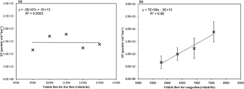
Ensemble mean dilution were determined for 1,000 vehicles/hr intervals and 5 km/hr intervals, and these average values were used to calculate EFs using CALINE4. Figure 4 provides the estimated UFP vehicle emission factor for LDVs as a function of mode of operation (free flow and congestion) using eq 2. Figure 4a presents the EFs for free flow conditions, and Figure 4b presents the EFs for congestion conditions. In Figure 4a, the vehicle emission factor for free flow conditions did not change with vehicle flow and was 1.5 × 10¹³ particles km⁻¹ vehicle⁻¹ for vehicle flow from 9,500 to 13,500 vehicles/hr. In Figure 4b, the vehicle EFs for congestion condition increased from 0.5 × 10¹³ to 2 × 10¹³ particles km⁻¹ vehicle⁻¹ when the flow increased from 5,500 to 7,500 vehicles/hr. Zhang et al. (2005) determined that the average emission factors from different studies were in the range of 10¹³ to 10¹⁴ particles km⁻¹ vehicle⁻¹.

Figure 4. Variation in emission factors (EF) with vehicle flow for (a) free flow and (b) congestion. The regression lines calculated from eq 2 using ensemble averages.

Determination of carbon dioxide concentrations

This section provides carbon dioxide (CO₂) measurements that are a function of traffic speed and mode of operation (congestion and free flow) for light-duty vehicles (LDVs) under real-world conditions. These measured concentrations can be compared with predicted concentrations derived from near-roadway meteorological and traffic measurements (5-min averages) and application of air quality dispersion models.

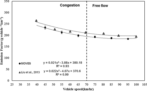
Emission factors of CO₂ from vehicles are determined using a motor vehicle emission model (MOVES2014) developed by the EPA that is based on pollutant emissions from dynamometer tests using a certain driving cycle and measurements of traffic volume and speed and mode of operation. Figure 5 shows CO₂ emission factor as a function of vehicle speed. The black spots are ensemble means of emission factors generated by using traffic data and the triangles are CO₂ emission factors reported in another study (Liu et al., 2013). Error bars in the figure represent the concentration variance around each ensemble mean value.

Figure 5. Emission factors of CO₂ generated from MOVES 2014 and Liu et al. (2013) as function of vehicle speed.

Figure 3 provides information on near-roadway measurements. The total CO₂ concentration varied between 440 and 625 ppm, with up to 170 ppm emitted from traffic (background subtracted). The background CO₂ concentration varied between 420 and 490 ppm. The large background concentrations of CO₂ and the large variation with time indicate the importance of measuring background concentrations and accounting for the impact that background concentrations have on the near-roadway environment.

When simultaneous measurements of meteorological conditions and emission factors from MOVES 2014 are available, it is possible to predict atmospheric concentrations of CO₂ for comparison with measured concentrations using eq 1. Dilution factor (DL) is calculated using a dispersion model, CALINE4, that describes the dilution due to roadway mixing and atmospheric dispersion of tail pipe emissions. Figure 6 provides a comparison of the modeled and measured CO₂ concentrations. The data are divided into congestion and free flow data sets. The vehicle CO₂ concentration increased for both modeled and measured CO₂ concentrations with vehicle speed when there was roadway congestion and decreased with vehicle speed when it was free flow.

Figure 6. Variation in individual measured and modeled vehicle carbon dioxide (CO₂) concentrations with vehicle speed for congestion and free flow. The regression line is for the ensemble means with 1 standard deviation.

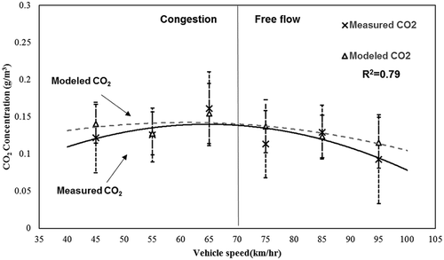
Figure 6 provides the best-fit line obtained by least square regression and the correlation coefficients for the averaged data. For congestion conditions, the CO₂ concentrations increased 20% when the average vehicle speed increased from 35 to 70 km/hr. There was a decrease of 30% in concentration when the average vehicle speed increased from 70 to 100 km/hr. These results are consistent because traffic flow decreases with increases in speed for free flow conditions. The overall results indicate that there is an increase in CO₂ with increases in speed for congestion conditions and a decrease in CO₂ with increases in speed for free flow conditions.

Comparison of measured and predicted ultrafine particulate concentrations using CALINE4 and AERMOD models

This section uses two air quality models—CALINE4 (California Line Source Dispersion Model, version 4) and AERMOD (American Meteorological Society/U.S. Environmental Protection Agency Regulatory Model)—to predict the ultrafine particulate concentrations near roadways for comparison with measured concentrations. CALINE4 is a specialized line source Gaussian dispersion model that predicts air pollutant concentrations near roadways using basic meteorology, surface roughness, traffic information, vehicle emission factors, and geometrical configuration of roadway links and receptors. Two different models are compared in this study because they are both used to predict concentrations near roadways and very little information is currently available in the literature comparing the performance of the models using the same input measurements. The comparison is needed because the models utilize different meteorological and roadway configuration information to predict near-roadway pollutant concentrations. Unlike other air dispersion models, CALINE4 includes a mixing cell that is defined as the region over the roadway and extends 3 m from the roadway edge. AERMOD is an atmospheric dispersion modeling system developed for the EPA for application to all types of pollutant sources. It is also a Gaussian dispersion model. The inputs to AERMOD include basic information used in CALINE4 and include additional meteorology data such as sensible heat flux, friction velocity, convective velocity, Monin-Obukhov length, Bowen ratio, and albedo. A line source in AERMOD can be simulated by the combination of finite area sources and volume sources. However, there is no mixing cell designation in AERMOD when it is used to analyze line sources.

The objective of this section is to compare measured air pollution concentrations near roadways with concentrations predicted from the models. Additionally, since AERMOD predictions have been determined to be very sensitive to surface roughness, a sensitivity analysis is conducted to determine the effect of changes in surface roughness on predicted concentrations. Seven receptor sites were used. Receptor A was only 2 m away from the road edge, which was regarded as in the mixing cell of the roadway. Receptors 1–5 were placed at a distance of 30, 60, 90, 150, and 200 m away from the downwind road edge in alignment perpendicular to the road. Background measurements were taken 100 m away from the road in the upwind direction.

Even though there is no mixing cell in AERMOD, the source was configured by an elevation of 0 m, a release height of 1.3 m, and an initial vertical dispersion coefficient of 1.2 m. Meteorology data in AERMOD were computed by AERMOD Model Formulations. Stability class was characterized by Monin-Obukhov lengths, selected as −42.6, −200.5, and −8888 m for Classes B, C, and D, respectively (Claggett, 2014). The surface roughness was selected as 0.05 m in both models based on local terrain conditions (Royal Aeronautical Society,1972). The east side of the roadway is located near Lake Michigan (300 m), with level terrain and short grass between the lake and the roadway. The west side of the roadway is a level sports field with short grass.

Figure 7 shows the downwind relative concentration gradients for the measured and predicted concentrations. The relative concentration is defined as the ratio of downwind to roadside concentration. The fitted trend lines in the figure indicate that the concentration exponentially decreases as the downwind distance increases. The correlation coefficients between the measured and predicted concentrations are all greater than 0.90. However, both AERMOD models have larger variances than CALINE4 and both of them are further away from the measured concentrations than CALINE4. Figure 8a compares the different model-predicted concentrations with measured concentrations when surface roughness is fixed at 0.05 m. The results show that the differences between model predictions and real measurements are a factor of 1.02, 1.15, and 1.16 for CALINE4, AERMOD volume source, and AERMOD area source. The Pearson correlations of individual data between models and measurements are 85.2%, 67.9%, and 64.7% for CALINE4, AERMOD volume source, and AERMOD area source, respectively. The Pearson correlations of average data are 97.6%, 88.8%, and 87.6% for each model.

Figure 7. Variation in relative concentrations with downwind distance for measurements; CALINE4 and AERMOD (Z₀ = 0.05 m).

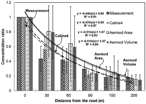
Figure 8. Comparison between model predictions and measurements when (a) Z₀ = 0.05 m and (b) Z₀ = 0.5 m for downwind relative concentration.

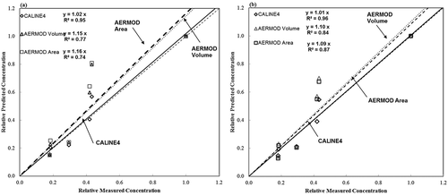
Figure 8 provides a comparison of measured and predicted differences when surface roughness values in the models are varied between 0.05 and 0.5 m. The model predictions vary from the perfect relationship (45° diagonal line) by 1%, 4%, and 6% for CALINE4, AERMOD volume, and AERMOD area, and there is very little change when surface roughness changes from 0.05 to 0.5 m (P value = 0.94, 0.98, and 0.92 for each model). This indicates that surface roughness does not play an important role in determining the relative downwind concentrations.

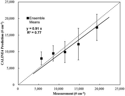
Figure 9 presents the impacts of surface roughness and atmospheric stability class on CALINE4 model from the near-roadway mixing cell concentration analysis. The difference between CALINE4 predictions and measurements is a factor of 0.91 and the correlation is 76%. Error bars in the figure represent the concentration variance around each ensemble mean value. The figure also shows that when the surface roughness values are changed from 0.01 to 0.5 m and stability class changed from Class B to Class D, there is no effect on the predicted mixing cell concentrations from the CALINE4 model.

Figure 9. CALINE4 predicted and near roadway measured mixing cell concentrations for different surface roughness and stability class condition.

Figure 10a and b show that AERMOD predicts significantly different concentrations of pollutant in the near-roadway mixing cell with changes in surface roughness. The model predicts a significant increase in concentration when the surface roughness decreases. Unlike CALINE4 model, the results indicate that AERMOD is much more sensitive to changes in surface roughness. When surface roughness is changed from 0.5 to 0.01 m, the predicted UFP concentrations increase by 250% and 210% for AERMOD volume source and AERMOD area source, whereas the similarity factor between prediction and measurement changes from 0.37 to 1.29 for AERMOD volume and from 0.46 to 1.41 for AERMOD area. A surface roughness value between 0.05 and 0.1 m seems to provide the best correlation between measured and modeled concentrations in this study, which reflects the local terrain conditions.

Figure 10. Comparison between AERMOD-predicted and near-roadway measured mixing cell concentrations for different surface roughness: (a) AERMOD volume; (b) AERMOD area.

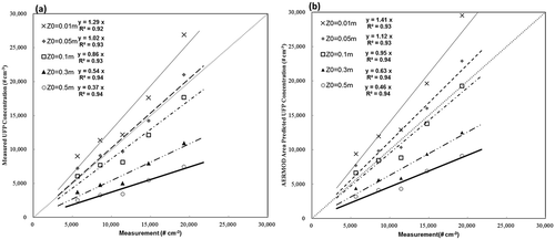
Analysis of the difference in predicted and measured near-roadway mixing cell concentrations for different stability classes in AERMOD demonstrates that there is an increase of about 15% for AERMOD volume source and AERMOD area source when stability class changes from Class B to Class D, which indicates that stability class does not dominate the UFP concentration change in AERMOD.

Discussion

Considering the dynamic nature of vehicle emissions and air quality near roadways, it is significant that similar EFs were obtained using measured and modeled data. The good agreement indicates that high-resolution, simultaneous measurements of air quality and meteorological and traffic conditions can be used to determine real-world, fleet-wide vehicle EFs as a function of vehicle mode of operation under actual driving conditions.

Comparison of measured and predicted concentrations using CALINE4 and AERMOD demonstrates that surface roughness does not play a dominant role in determining the relative concentration decrease with downwind distance for both CALINE4 and AERMOD models. When using CALINE4 to predict air quality levels in the mixing cell, changes in surface roughness and stability class have no effect on the predicted concentrations. However, when using AERMOD to predict air quality in the mixing cell, changes in surface roughness have a significant effect on the predicted concentrations.

Summary

This paper demonstrates that near-roadway monitoring can provide significant information on the dynamic process related to the emission and mixing of pollutants near roadways due to turbulence introduced by moving vehicles. The key finds are as follows.

Real-world fleet emission factors as a function of vehicle mode of operation can be determined from near-roadway monitoring of pollutant concentrations, traffic flow rate, vehicle speed, and estimates of pollutant dilution due to turbulent mixing induced by the moving vehicles. Air pollution concentrations near roadways can be predicted using dispersion models when emission factors are available from MOVES 2014 and meteorological and traffic conditions are measured near roadways. The turbulent mixing induced by moving vehicles can be determined from application of either CALINE4 or AERMOD dispersion model. However, AERMOD requires significantly more input information on the meteorological and near-roadway conditions and is sensitive to surface roughness. Future near-roadway monitoring efforts need to be directed at determining the effect that turbulent-induced mixing due to trucks has on pollutant concentrations near roadways. This is important because trucks generate significant addition turbulence near roadways even though they typically represent only 5–10% of the total vehicle flow.

Acknowledgment

We are immensely grateful to Air Quality Measurement Methods and Technology Conference (2016, Chapel Hill, North Carolina) committee for their comments on an earlier version of the manuscript.

Funding

This research was supported by the Air and Waste Management Association (A&WMA).

Additional information

Funding

This research was supported by the Air and Waste Management Association (A&WMA).

Notes on contributors

Dongqi Wen

Dongqi Wen, PhD in Environmental Engineering, is an Air Quality Specialist, Douglas County Health Department, Omaha, Nebraska, USA.

Wenjuan Zhai

Wenjuan Zhai, PhD in Environmental Engineering, is a Staff Engineer, RK & Associates, Inc., Warrenville, Illinois, USA.

Sheng Xiang

Sheng Xiang and Zhice Hu are PhD candidates in Environmental Engineering. Illinois Institute of Technology, Chicago, Illinois, USA.

Tongchuan Wei

Tongchuan Wei, is a PhD Candidate in Environmental Engineering, North Carolina State University, Raleigh, North Carolina, USA.

Kenneth E. Noll

Kenneth E. Noll, PE, PhD, Professor, Illinois Institute of Technology, Chicago, Illinois, USA.

References

- Claggett, M. 2014. Comparing predictions from the CAL3QHCR and AERMOD models for highway applications. Transport. Res. Rec. 2428:18–26. doi: 10.3141/2428-03.
- E Instruments. 2015. Products AQ Pro Web site, 2015. http://www.e-inst.com/environmental-iaq/products-AQ-Pro (accessed December 6, 2015).
- Fruin, S., D. Westerdahl, T. Sax, and C. Sioutas. 2008. Fine PM. Measurements and predictors of on-road ultrafine particle concentrations and associated pollutants in Los Angeles. Atmos. Environ. 42:207–19. doi: 10.1016/j.atmosenv.2007.09.057.
- Iijima, S.J. 1985. Electron microscopy of small particles. J. Electron Microsc. 34:249–65. doi:10.1093/oxfordjournals.jmicro.a050518
- Kirchstetter, T., R. Harley, N. Kreisberg, M. Stolzenburg, and S. Hering. 1999. On-road measurement of fine particle and nitrogen oxide emissions from light- and heavy-duty motor vehicles. Atmos. Environ. 33:2955–68. doi:10.1016/S1352-2310(99)00089-8
- Kumar, P., A. Robins, S. Vardoulakis, and R. Britter. 2010. A review of the characteristics of nanoparticles in the urban atmosphere and the prospects for developing regulatory controls. Atmos. Environ. 44:5035–52. doi:10.1016/j.atmosenv.2010.08.016
- Liu, H., X. Chen, Y. Wang, and S. Han. 2013. Vehicle emission and near-road air quality modeling for Shanghai, China. Transport. Res. Rec. 2340:38–48. doi: 10.3141/2340-05.
- Mannering, F.L., and S.S.Washburn. 2013. Principles of Highway Engineering and Traffic Analysis, 5th ed. Hoboken, NJ: John Wiley.
- Morawska, L., Z. Ristovski, E. Jayaratne, D. Keogh, and X. Ling. 2008. Ambient nano and ultrafine particles from motor vehicle emissions: Characteristics, ambient processing and implications on human exposure. Atmos. Environ. 42:8113–38. doi:10.1016/j.atmosenv.2008.07.050
- National Ambient Air Quality Standards (NAAQS). 2015. U.S. Environmental Protection Agency Web site. http://www3.epa.gov/ttn/naaqs/criteria.html ( accessed December 6, 2015).
- Palmgren, F., R. Berkowicz, A. Ziv, and O. Hertel. 1999. Actual car fleet emissions estimated from urban air quality measurements and street pollution models. Sci. Total Environ. 235:101–9. doi:10.1016/S0048-9697(99)00196-5
- Royal Aeronautical Society. 1972. Characteristics of Wind Speed in the Lower Layers of the Atmosphere near the Ground: Strong Winds (Neutral Atmosphere). Engineering Science Data. Unit No.: 72026. London, UK: Royal Aeronautical Society.
- Technical Support, Inc. 2002. Model 3007 Condensation Particle Counter: Operation and Service Manual, TSI Incorporated, Shoreview, MN USA. http://www-cirrus.ucsd.edu/pages/instruments/Manual-3007.pdf (accessed August 1, 2014).
- TSI. 2013. P-TRAK Ultrafine Particle Counter Model 8525 Operation Service Manual. TSI Products web site. http://www.tsi.com/uploadedFiles/_Site_Root/Products/Literature/Manuals/Model-8525-P-Trak-1980380.pdf (accessed December 6, 2015).
- U.S. Environmental Protection Agency. 2014. Motor Vehicle Emission Simulator (MOVES): User Guide for MOVES. EPA-420-B-14-055. Washington, DC: U.S. Environmental Protection Agency, Assessment and Standards Division, Office of Transportation and Air Quality. www.epa.gov/oms/models/moves/documents/420b14055.pdf (accessed October 6, 2015).
- Venkatram, A., V. Isakov, E. Thoma, and R.W. Baldauf. 2007. Analysis of air quality data near roadways using a dispersion model. Atmos Environ. 41:9481–97. doi: 10.1016/j.atmosenv.2007.08.045.
- Westerdahl, D., S. Fruin, T. Sax, P.M. Fine, and C. Sioutas. 2005. Mobile platform measurements of ultrafine particles and associated pollutant concentrations on freeways and residential streets in Los Angeles. Atmos. Environ. 39:3597–610. doi:10.1016/j.atmosenv.2005.02.034
- Zhang, K.M., and A.S. Wexler. 2004. Evolution of particle number distribution near roadways—Part I: Analysis of aerosol dynamics and its implications for engine emission measurement. Atmos. Environ. 38:6643–53. doi:10.1016/j.atmosenv.2004.06.043
- Zhang, K. M., A.S. Wexler, D.A. Niemeier, Y. Zhu, W.C. Hinds, and C. Sioutas. 2005. Evolution of particle number distribution near roadways. Part III: Traffic analysis and on-road size resolved particulate emission factors. Atmos. Environ. 39:4155–66. doi:10.1016/j.atmosenv.2005.04.003
- Zhu, Y., W.C. Hinds, S. Kim, and C. Sioutas. 2002a. Concentration and size distribution of ultrafine particles near a major highway. J. Air Waste Manage. Assoc. 52:1032–42. doi:10.1080/10473289.2002.10470842
- Zhu, Y.; W.C. Hinds, S. Kim, S. Shen, and C. Sioutas. 2002b. Study of ultrafine particles near a major highway with heavy-duty diesel traffic. Atmos. Environ. 36:4323–35. doi: 10.1016/S1352-2310(02)00354-0
- Zhu, Y., W.C. Hinds, M. Krudysz, T. Kuhn, J. Froines, and C. Sioutas. 2005. Penetration of freeway ultrafine particles into indoor environments. J. Aerosol Sci. 36:303–22. doi:10.1016/j.jaerosci.2004.09.007