Alternate approaches for assessing impacts of oil sands development on air quality: A case study using the First Nation Community of Fort McKay

ABSTRACT

Previous analyses of continuously measured compounds in Fort McKay, an indigenous community in the Athabasca Oil Sands, have detected increasing concentrations of nitrogen dioxide (NO₂) and total hydrocarbons (THC), but not of sulfur dioxide (SO₂), ozone (O₃), total reduced sulfur compounds (TRS), or particulate matter (aerodynamic diameter <2.5 μm; PM_2.5). Yet the community frequently experiences odors, dust, and reduced air quality. The authors used Fort McKay’s continuously monitored air quality data (1998–2014) as a case study to assess techniques for air quality analysis that make no assumptions regarding type of change. Linear trend analysis detected increasing concentrations of higher percentiles of NO₂, nitric oxide (NO), and nitrogen oxides (NO_x), and THC. However, comparisons of all compounds between an early industrial expansion period (1998–2001) and current day (2011–2014) show that concentrations of NO₂, SO₂, THC, TRS, and PM_2.5 have significantly increased, whereas concentrations of O₃ are significantly lower. An assessment of the frequency and duration of periods when concentrations of each compound were above a variety of thresholds indicated that the frequency of air quality events is increasing for NO₂ and THC. Assessment of change over time with odds ratios of the 25th, 50th, 75th, and 90th percentile concentrations for each compound compared with an estimate of natural background variability showed that concentrations of TRS, SO₂, and THC are dynamic, higher than background, and changes are nonlinear and nonmonotonic. An assessment of concentrations as a function of wind direction showed a clear and generally increasing influence of industry on air quality. This work shows that evaluating air quality without assumptions of linearity reveals dynamic changes in air quality in Fort McKay, and that it is increasingly being affected by oil sands operations.

Implications: Understanding the nature and types of air quality changes occurring in a community or region is essential for the development of appropriate air quality management policies. Time-series trending of air quality data is a common tool for assessing air quality changes and is often used to assess the effectiveness of current emission management programs. The use of this tool, in the context of oil sands development, has significant limitations, and alternate air quality change analysis approaches need to be applied to ensure that the impact of this development on air quality is fully understood so that appropriate emission management actions can be taken.

Introduction

Fort McKay is an indigenous community (First Nation and Métis) located in the northeast corner of the Province of Alberta, Canada (see Figure 1) with an in-community population of approximately 565 (Statistics Canada, 2015). Its location places it in the center of one of the world’s largest oil deposits (Alberta Energy, 2016).

Table 1. Bitumen and synthetic crude production (million m³) by facility and year for oil sands developments north of Fort McMurray with the direction from the facility to Fort McKay, and total bitumen and synthetic crude production for the Athabasca Oil Sands.

Year	Suncor base plant	Suncor base plant	Syncrude Mildred Lake	Syncrude Mildred Lake	Syncrude Aurora North	Shell Muskeg River	Suncor MacKay River	Suncor Firebag	CNRL Horizon	CNRL Horizon	Shell JP	Imperial Kearl	Total	Total
Product	SC	MB	SC	MB	MB	MB	BIT	BIT	SC	MB	MB	MB	BIT	SC
1998	4.06	6.56	12.32	14.64									21.20	16.38
1999	3.71	7.58	13.06	15.83									23.40	16.77
2000	4.42	8.29	11.95	13.34									21.63	16.36
2001	3.76	8.89	11.11	12.30	2.16								23.35	14.86
2002	8.05	15.66	13.54	11.40	4.27	0.03	0.07						31.42	21.59
2003	8.14	15.71	12.51	10.08	4.73	4.99	0.62						36.14	20.65
2004	12.82	15.74	14.08	8.47	8.20	8.46	0.96	0.64					42.48	26.90
2005	9.37	11.36	12.86	7.27	7.95	9.77	1.24	1.10					38.68	22.23
2006	14.95	17.63	15.07	7.33	10.71	8.44	1.27	1.95					47.33	30.03
2007	13.63	15.49	17.98	9.37	11.96	8.73	1.20	2.14					48.89	31.61
2008	13.46	14.43	17.04	9.55	10.11	7.83	1.46	2.19	0.04	0.06			45.62	30.54
2009	16.53	16.80	16.55	8.39	11.00	8.10	1.70	2.83	3.03	3.59			52.41	36.11
2010	15.00	15.44	17.32	8.91	11.37	6.22	1.83	3.11	5.34	6.34	1.49		54.70	37.66
2011	16.71	16.70	16.93	8.64	11.48	7.39	1.74	3.45	2.35	2.79	4.79		56.99	36.00
2012	16.41	15.49	16.90	8.83	10.70	7.46	1.57	6.04	5.05	5.99	5.64		61.71	38.36
2013	16.74	15.65	15.92	8.58	10.38	7.93	1.65	8.34	5.84	6.80	5.85	1.45	66.63	38.51
2014	17.18	15.92	15.16	7.60	10.42	7.67	1.55	10.03	6.47	7.53	6.46	4.62	71.79	38.82
WD to Fort McKay	S-SSE	S-SSE	S-SW	S-SW	NE	ENE-E	WSW	E	N-NNE	N-NNE	E	ENE

Note. CNRL = Canadian Natural Resources Ltd; JP = Jack Pine; SC = synthetic crude; MB = mined bitumen; Bit = bitumen.

Table 2. Thresholds for determining poor air quality events.

Compound	One-hour threshold	Source	Reason
NO2	159 ppb	AAAQO	Odor perception
NO2	92 ppb	LARP AMF—Level 4 trigger	Calculation based on relationship between 99th percentile and maximum values at all WBEA continuous monitoring stations
	62 ppb	LARP AMF—Level 3 trigger
	30 ppb	LARP AMF—Level 2 trigger
SO2	172 ppb	AAAQO	Pulmonary function
SO2	36 ppb	LARP AMF—Level 4 trigger	Calculation based on relationship between 99th percentile and maximum values at all WBEA community monitoring stations
	24 ppb	LARP AMF—Level 3 trigger
	12 ppb	LARP AMF—Level 2 trigger
THC	2 ppm		Odor perception
	5.9 ppm	n-Hexane AAAQO	Derived from 24-hr California objective
TRS	2 ppb		Odor perception
	10 ppb	H2S AAAQO	Odor perception
O3	82 ppb	AAAQO	Pulmonary function
	50 ppb	CAAQM Yellow Management Level	Derived from Canada-wide standard based on daily maximum 8-hr values
PM2.5	80 µg/m^3	AAAQG	Derived from Canada-wide standard

Note. AAAQO = Alberta Ambient Air Quality Objectives; LARP AMF = Lower Athabasca Regional Plan Air Management Framework; AAAQG = Alberta Ambient Air Quality Guidelines.

*___.

Table 3. Results of Theil-Sen trend analysis of compound concentration percentiles from 1998 to 2014.

Compound	Percentile	Trend	P
NO	50		0.23
	75	Increasing	0.052
	90	Increasing	0.012
	98	Increasing	0.00034
NOx	50	Increasing	0.019
	75	Increasing	0.0020
	90	Increasing	0.00046
	98	Increasing	3.2 × 10^−5
NO2	50	Increasing	0.011
	75	Increasing	8.9 × 10^−5
	90	Increasing	0.00011
	98	Increasing	2.2 × 10^−5
SO2	50		0.36
	75		0.43
	90		0.25
	98		0.65
TRS	50		0.34
	75		0.51
	90		0.54
	98		0.27
THC	50	Increasing	0.020
	75	Increasing	0.047
	90		0.38
	98		0.56
O3	50	Decreasing	0.070
	75		1
	90		0.97
	98		0.41
PM2.5	50		0.71
	75		0.93
	90		0.91
	98		0.30

Note. Theil-Sen slopes and significance were calculated using the function sens.slope in the “trend” package (Pohlert, 2017) in R (R Core Team, 2014). Those results that are significant (P < 0.05) are shown in bold, for those significant at a Bonferroni-corrected α (P < 0.00156) are shaded; strongly nonsignificant results are blank.

Table 4. Summary of the Mann-Whitney U tests of air quality changes between the early industrial (1998–2001) and late industrial (2011–2014) periods.

		Wind directions and assessment periods
Com pound	Change and trend parameters	N-ENE (25°–80°)	E (80°–100°)	S-SSE (150°–180°)	S-SW (180°–225°)	WSW (230°–250°)	N-NNW (330°–360°)*	All others combined (0°–25°, 100°–150°, 225°–230°, and 250°–330°)	All wind directions
SO2	Mean conc. early (ppb)	1.43	1.80	3.33	1.20	0.48	0.53	0.81	1.28
	Δ in mean conc. (ppb)	−0.55	−0.63	0.49	0.18	0.18	0.09	0.13	0.12
	% Δ in mean conc. (ppb)	−39%	−35%	15%	15%	38%	17%	16%	10%
	P	↓ 0.037	↓ <0.0001	↑ <0.0001	↑ <0.0001	↑ <0.0001	↑ <0.0001	↑ <0.0001	↑ <0.0001
	Δ in ave. emissions (t/yr)	299	492	6452	−28,319	160	3234	0	−17,682
	Δ in ave. production (m^3/yr)	19,873,000	14,120,000	20,539,000	−1,492,000	1,629,000	12,560,000	0	67,229,000
TRS	Mean conc. early (ppb)	0.28	0.34	0.68	0.64	0.30	0.31	0.32	0.44
	Δ in mean conc. (ppb)	0.11	0.07	0.06	0.04	0.11	0.06	0.09	0.07
	% Δ in mean conc. (ppb)	41%	21%	8%	7%	37%	18%	29%	16%
	p	↑ <0.0001	↑ <0.0001	↑ <0.0001	↑ <0.0001	↑ <0.0001	↑ <0.0001	↑ <0.0001	↑ <0.0001
	Δ in ave. emissions (t/yr)	2	9	123	47	0	20	0	201
	Δ in ave. production (m^3/yr)	19,873,000	14,120,000	20,539,000	−1,492,000	1,629,000	12,560,000	0	67,229,000
NO2	Mean conc. early (ppb)	1.91	3.57	7.48	7.71	2.00	2.79	2.71	4.45
	Δ in mean conc. (ppb)	5.19	3.15	2.84	3.63	2.99	3.20	2.46	2.82
	% Δ in mean conc. (ppb)	37%	113%	263%	212%	67%	87%	110%	158%
	P	↑ <0.0001	↑ <0.0001	↑ <0.0001	↑ <0.0001	↑ <0.0001	↑ <0.0001	↑ <0.0001	↑ <0.0001
	Δ in ave. NOx emissions (t/yr)	14,982	7889	10,784	−3769	492	6324	0	36,702
	Δ in ave. production (m^3/yr)	19,873,000	14,120,000	20,539,000	−1,492,000	1,629,000	12,560,000	0	67,229,000
THC	Mean conc. early (ppm)	1.835	1.839	2.007	2.015	1.801	1.844	1.837	1.896
	Δ in mean conc. (ppm)	0.15	0.16	0.10	0.12	0.23	0.11	0.16	0.14
	% Δ in mean conc. (ppm)	8%	8%	5%	6%	13%	6%	9%	8%
	P	↑ <0.0001	↑ <0.0001	↑ <0.0001	↑ <0.0001	↑ <0.0001	↑ <0.0001	↑ <0.0001	↑ <0.0001
	Δ in ave. VOC emissions (t/yr)	13,832	1997	2288	−3685	48	28,845	0	43,323
	Δ in ave. production (m^3/yr)	19,873,000	14,120,000	20,539,000	−1,492,000	1,629,000	12,560,000	0	67,229,000
O3	Mean conc. early (ppb)	26.59	27.22	21.30	16.73	23.97	19.83	21.99	21.05
	Δ in mean conc. (ppb)	0.11	0.46	−0.37	−2.34	−4.95	−1.31	−0.67	−0.88
	% Δ in mean conc. (ppb)	0.4%	1.7%	−1.8%	−14.0%	−20.7%	−6.6%	−3.1%	−4.2%
	P	↔ (P = 0.784)	↔ (P = 0.729)	↓ <0.001	↓ <0.0001	↓ <0.0001	↓ <0.0001	↓ <0.0001	↓ <0.0001
	Δ in ave. precursor (NOxand THC) emissions (t/yr)	28,814	9886	13,072	−7454	540	35,169	0	80,025
	Δ in ave. production (m^3/yr)	19,873,000	14,120,000	20,539,000	−1,492,000	1,629,000	12,560,000	0	67,229,000
PM2.5	Mean conc. early (µg/m^3)	6.69	7.82	9.32	7.35	5.04	5.50	5.92	6.71
	Δ in MEAN COnc. (µg/m^3)	2.64	0.62	−0.39	1.40	1.98	1.43	1.88	1.62
	% Δ in mean conc. (µg/m^3)	39%	8%	−4%	19%	39%	26%	32%	24%
	P	↑ <0.0001	↑ <0.0001	↑ <0.0001	↑ 0.009	↑ 0.008	↑ 0.049	↑ <0.0001	↑ <0.0001
	Δ in ave. emissions (t/yr)	2489	402	1170	545	24	444	0	5074
	Δ in ave. production (m^3/yr)	19,873,000	14,120,000	20,539,000	−1,492,000	1,629,000	12,560,000	0	67,229,000

Note. Tests that are significant (P < 0.05) are in bold. Also shown are the absolute changes and percent changes of mean compound concentrations and the change in production and emissions between time periods.

Table 5. Results of Spearman rank correlation analysis of compound concentration percentiles and production of bitumen or synthetic crude from 1998 to 2014.

Compound	Explanatory variable	Percentile	r coefficient	P
NO2	Bitumen	50	0.502	0.0403
	Synthetic crude	50	0.532	0.0279
	Bitumen	98	0.839	2.54 × 10^−5
	Synthetic crude	98	0.802	1.08 × 10^−4
SO2	Bitumen	50	0.364	0.151
	Synthetic crude	50	0.355	0.162
	Bitumen	98	−0.0143	0.957
	Synthetic crude	98	−0.526	0.841
TRS	Bitumen	50	0.242	0.349
	Synthetic crude	50	0.213	0.413
	Bitumen	98	0.142	0.586
	Synthetic crude	98	0.296	0.248
THC	Bitumen	50	0.662	0.00381
	Synthetic crude	50	0.632	0.00647
	Bitumen	98	0.110	0.674
	Synthetic crude	98	0.206	0.429
O3	Bitumen	50	−0.430	0.0846
	Synthetic crude	50	−0.499	0.0414
	Bitumen	98	0.274	0.288
	Synthetic crude	98	0.306	0.232
PM2.5	Bitumen	50	−0.0405	0.877
	Synthetic crude	50	0.0380	0.885
	Bitumen	98	0.303	0.237
	Synthetic crude	98	0.298	0.245

Note. Significance is calculated using the function cor.test in R (R Core Team, 2014). Those results that are significant (P < 0.05) are bolded; those significant at a Bonferroni-corrected α (P < 0.00208) are shaded.

Table 6. Results of Spearman correlation analysis to assess whether estimated emissions correlate with percentiles of ambient concentrations in Fort McKay.

Compound	Percentile	Correlation coefficient	P
NOx	50	0.431	0.0854
	98	0.825	4.50 × 10^−5
SO2	50	−0.550	0.0221
	98	0.374	0.172
VOC/THC	50	0.354	0.164
	98	−0.0524	0.842
PM2.5	50	−0.081	0.757
	98	0.213	0.412

Note. Significance is calculated using the function cor.test in R (R Core Team, 2014). Those results that are significant (P < 0.05) are in bold, whereas those significant at a Bonferroni-corrected α (P < 0.00625) are shaded.

Table 7. Summary statistics of poor air quality events, from 1998 to 2014.

Compound	Threshold	Number of events	Median duration (hr)	Maximum duration (hr)	Total hours in exceedance
NO2	LARP Level 2: 30 ppb	588	2	18	1604
	LARP Level 3: 62 ppb	0	0	0	0
	LARP Level 4: 92 ppb	0	0	0	0
	AAAQO: 159 ppb	0	0	0	0
SO2	LARP Level 2: 12 ppb	1175	2	14	2755
	LARP Level 3: 24 ppb	462	1	10	815
	LARP Level 4: 36 ppb	205	1	6	323
	AAAQO: 172 ppb	1	1	1	1
TRS	H2S AAQO: 10 ppb	46	2	9	96
	Odor detection: 2 ppb	1412	2	60	4823
THC	AAAQO n-Hexane: 5.96 ppm	14	1	10	36
	Odor detection: 2 ppm	4849	4	1429	51473
O3	AAAQO: 82 ppb	9	1	2	13
	CAAQM Yellow: 50 ppb	503	3	17	2182
PM2.5	AAAQG: 80 µg/m^3	92	2.5	20	349

Table 8. Results of Theil-Sen trend analysis of number of exceedances from 1998 to 2014.

Compound	Threshold	Trend	P
NO2	Level 2—30 ppb	Increasing	3.1 × 10^−5
SO2	Level 2—12 ppb		0.43
	Level 3—24 ppb		0.90
	Level 4—36 ppb		0.34
TRS	10 ppb		0.43
	2 ppb		0.43
THC	2 ppm	Increasing	0.0074
O3	80 ppb		Insufficient data
	50 ppb		0.25
PM2.5	80 µg/m^3	Increasing	0.091

Note. Theil-Sen slope and significance calculated using procedure sens.slope in package “trends” (Pohlert, 2017) in R (R Core Team, 2014). Significant results (P < 0.05) are in bold. Those results significant at a Bonferroni-corrected α (P < 0.005) are shaded. Strongly nonsignificant results are blank.

Table 9. Average emissions and percent change in emissions of the noted parameters for the noted periods (tonnes/yr).

Period	SO2	NOx	PM2.5	VOC	RSC (H2S, CS₂ and COS as H₂S)
1998–2001	97,276	36,573	1158	26,495	141
2011–2014	78,262	70,562	5291	54,961	340
% Change	−20	93	357	107	140

Figure 1. Oil sands regions in northeastern Alberta. Map showing the Peace, Cold Lake, and Athabasca oil sands regions, and the location of Fort McKay and the closest major urban center, Fort McMurray. Fort McKay is located at latitude 57.163, longitude −111.618.

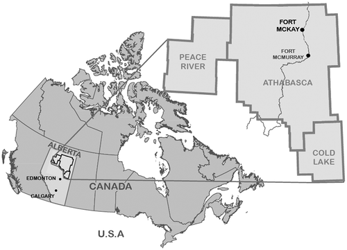
Figure 2. The locations, names, and types of oil sands developments near Fort McKay, as of 2015.

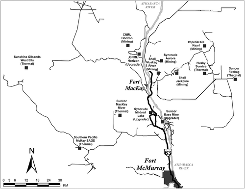
Figure 3. Analysis of exceedances of poor air quality thresholds in Fort McKay. Shown are box plots of exceedance duration. The black line (Hours past threshold) indicates the total number of hours in exceedance, and the gray line (Number of events) indicates the total number of exceedance events. SO₂ and NO₂ exceedance levels are based on Lower Athabasca Regional Plan Air Quality Management Framework, and particulate matter exceedance level is based on an Alberta Ambient Air Quality Objective (AAAQO). The threshold of 2 ppb for TRS is based on the level of odor detection (Nagata, 2003). The thresholds for THC are based on an assumed odor threshold of 2 ppm, which translates to a nonmethane hydrocarbon level of 200 ppb. The threshold for O₃ of 50 ppm is based on the Canadian Ambient Air Quality Standards (CAAQS) Management Level Yellow of 50 ppm.

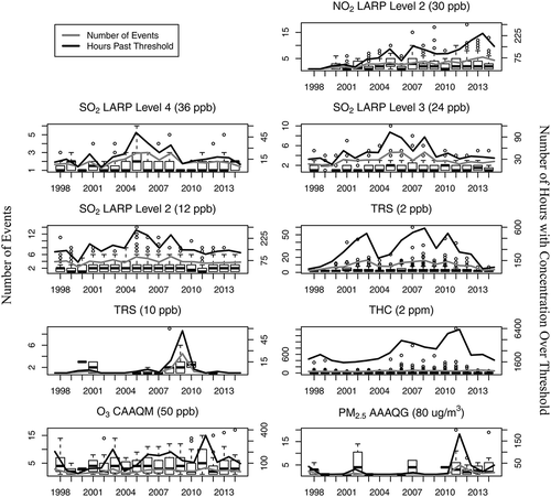
Figure 4. Odds ratios of percentiles of ambient concentrations of different compounds. Shown are 99.95% confidence intervals. The odds ratios are calculated by comparing the observed with expected fractions of air quality measurements above each percentile. The dotted line represents an odds ratio of 1, indicating no increase in observations above that percentile. Note differing scales of y-axes.

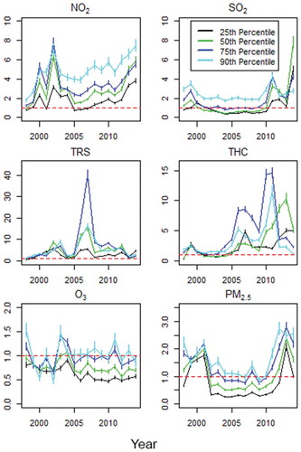
Figure 5. Henry plots of mean hourly ambient concentrations of air contaminants as a function of wind direction at Fort McKay. Shown are plots for the early industrial period (1998–2001) and late industrial period (2011–2014), with 99.99% confidence intervals. Henry plots were calculated using a modified Gaussian kernel with a 5° sliding window.

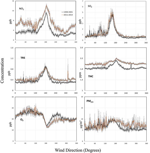
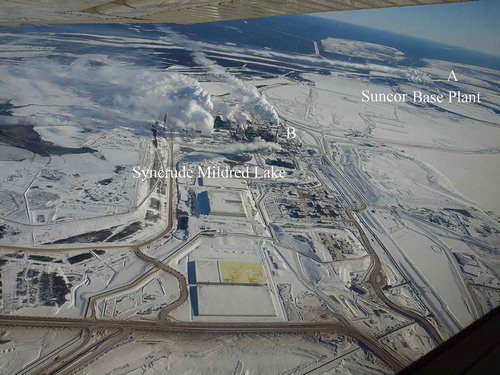
Figure 6. Aerial photo showing dispersion of plumes from Suncor base plant and Syncrude Mildred Lake. In winter, the condensing of the water vapor in emission allows a visual observation of the dispersion patterns of different emission sources. Suncor Base Plant’s flue gas desulfurization stack is 137 m high and has a base level of 255 m, whereas Syncrude’s main stack is 183 m high and has a base level of 304 m. Thus, emissions from Suncor’s stack are often trapped in the Athabasca Valley and subject to the predominant north-south valley winds, whereas Syncrude’s emissions (B) may escape this ground-level wind pattern. Photo: Ryan Abel.

Oil sands developments are a source of nitrogen oxide (NO_x), sulfur dioxide (SO₂), fine particulate (aerodynamic diameter <2.5 μm; PM_2.5), volatile organic compound (VOC), carbon monoxide (CO), reduced sulfur compound (RSC), and polycyclic aromatic compound (PAC) emissions (Davies et al., 2012; Galarneau et al., 2014; Kelly et al., 2009; Marson, 2015; Small et al., 2015; Trace Metals Air Contaminant Working Group [TMAC], 2001, 2003; Wang et al., 2015a, 2015b ; Zhang et al., 2016). Adverse short- and/or long-term health effects are associated with exposure to these types of air contaminants, often studied in isolation, and for NO₂ and PM_2.5 it is uncertain whether there is an exposure level that does not contribute to adverse health effects (Agency for Toxic Substances and Disease Registry, 1995; World Health Organization, 2000; 2006, 2013; U.S. Environmental Protection Agency [EPA], 2008, 2009, 2010, 2013; Bernstein et al., 2004; Pope and Dockery, 2006; Craig et al., 2008; International Agency for Research on Cancer, 2016).

Fort McKay’s proximity to the mining and upgrading center of oil sands development (see Figure 2) leaves it vulnerable to a variety of environmental impacts (Spink and Abel, 2015), including air quality impacts (Gossel et al., 2010).

The issues of air quality deterioration, quality-of-life impacts, and possible adverse direct and indirect health effects are major concerns to the residents of Fort McKay (Dennis et al., 2015; Fort McKay Industy Relations Corporation, 2010; Gossel et al., 2010). Whether air quality data support these concerns has been, and continues to be, a matter of debate. For example, in 2010, one report on air quality in the oil sands region reported that air pollution “exceedances” had increased from 47 in 2004 to 1556 in 2009 (Environmental Defence Canada, 2010), with almost all these exceedances related to hourly and daily total reduced sulfur compounds/hydrogen sulfide (TRS/H₂S) levels (Wood Buffalo Environmental Association, 2009), whereas a paper the same year concluded that increasing oil sands development was having minimal to no impact on air quality trends of SO₂, CO, PM_2.5, O₃, and TRS in the communities of Fort McMurray, Fort McKay, and Fort Chipewyan (Kindzierski, 2010). Subsequent simple parametric linear trend analysis (Bari and Kindzierski, 2015; Kindzierski and Bari, 2011) indicated that changes to air quality in communities in the Athabasca Oil Sands Region (AOSR) are limited to small changes in median nitric oxide (NO), higher percentiles of NO₂, and median and higher percentiles of THC, whereas a comparison of four communities using annual median and geometric means showed an increase in THC and a decrease in NO₂ (Bari and Kindzierski, 2016). Thus, trend analyses using different measures of central tendency can give different conclusions, which suggests that these complex data are not conducive to these types of analyses. The consideration of percentiles can clarify some of these issues, by identifying trends in extreme measures as well as measures of central tendency (Cooper et al., 2012). However, the assumption remains that only monotonic, linear trends are meaningful. Although there continues to be uncertainty regarding the magnitude and significance of air quality impacts associated with oil sands development, and the methodologies for assessing changes in air quality are evolving, there is a general recognition that oil sands development–related odor impacts are an air quality issue in the region and for Fort McKay (MacEachern, 2010; O’Brien et al., 2012; Percy et al., 2012; Wood Bufffalo Environmental Association, 2013). Different approaches to examining air quality data in Fort McKay might reveal patterns that have previously been undescribed.

In the assessment of the possible impacts of oil sands emissions on air quality in the Athabasca Oil Sands Region (AOSR), and in communities located in the AOSR such as Fort McKay, the principal statistical tools used to date have been time-series air quality trend analysis using parametric (simple linear regression) or nonparametric (Theil-Sen’s) tests (Bari and Kindzierski, 2015; Bari et al., 2016; Faisel et al., 2006; Kindzierski, 2010; Kindzierski and Bari, 2011; Kindzierski et al., 2009; Xu et al., 2006). The most recent and detailed multi-air-contaminant time-series trending of air quality in Fort McKay (Bari and Kindzierski, 2015) used ordinary parametric linear regression to assess air quality changes over time (1998–2012) at air quality monitoring stations throughout the AOSR. These authors (Bari and Kindzierski, 2015) found that in Fort McKay, only NO₂ and THC levels showed consistent but small increasing levels over this 15-yr period. Recent trend analysis of NO₂ and SO₂ using satellite-based spectrometry over the AOSR found a significant and much higher increasing trend in NO₂ and relatively constant levels in SO₂ over the period 2005–2014, consistent with ground-level monitoring (McLinden et al., 2016); however, none of these analyses considered other types of air quality change.

Although air quality trend analyses to date, using either measures of central tendency or percentiles, report little to no change in air quality in Fort McKay, the residents of this community report frequent occurrences of poor air quality, odors, and dust in the community (Alberta Energy Regulator and Alberta Health, 2016; Teck Resources Limited, 2015a). Because emission types, emission spatial and temporal variability, regional topography, land use, meteorology, climate, seasonality, and atmospheric processes can all impact local air quality (Chan and Yao, 2008; Fann et al., 2009; Jerrett et al., 2007; Mayer, 1999), detecting trends and changes and attributing cause is exceedingly complex. Variability in industrial processes, wildfires, and wind patterns result in both short- and longer-term nonlinear changes in air quality. Oil sands emission sources are varied: tall and short stacks, mine fleets operating at or below ground level in changing locations, and fugitive emissions from plant sites, mines, and tailings ponds (Davies, 2012) each have their own emission and dispersion characteristics. Wind speed and direction variability significantly influence air quality at a location (Henry, 2008), and these can vary by elevation and year. Examining whether air quality data exhibit linear trends over time is a blunt tool that simply looks for one type of change (Hirsh et al., 1991; Helsel and Hirsh, 2002); its popularity might, in fact, obscure nonlinear changes in air quality, such as nonmonotonic changes in concentrations (Wu et al., 2007), or the frequency and intensity of short episodes of poor air quality.

In this work, we focus on air quality issues at the air monitoring station in Fort McKay because this is the community most impacted by oil sands development air emissions (Gossel et al., 2010), and it allows us to assess different techniques for evaluating air quality data. We assessed long-term air quality changes and trends using traditional statistical approaches, including linear nonparametric analysis, comparison of median ambient concentrations in early development period versus the late development period, and correlations between oil sands production and ambient air quality, to provide a backdrop of results commonly found by traditional approaches. To gain a better understanding of events where there are odors in the community, we then assessed the frequency, magnitude, and duration of times where ambient concentrations of certain substances were above a variety of thresholds. As an alternative to linear trending, we examined air quality changes over time using methods that did not assume an underlying distribution or form of change by calculating odds ratios for each percentile against an assumed background. Finally, to assess whether industry could be identified as a source, and the possible magnitude and change associated with this source, we applied nonparametric regression approaches to wind direction to determine whether ambient concentrations were related to oil sands emissions.

Methods

Measures of air quality and meteorological parameters

Air quality is measured continuously by the Wood Buffalo Environmental Association (WBEA) at air quality stations throughout the AOSR. The community air quality station in Fort McKay, Bertha Ganter (AMS1; latitude: 57.163, longitude: −111.618), measures numerous chemical parameters as well as wind speed, wind direction, relative humidity, and solar radiation (10 m elevation) and temperature (at 2 m and 10 m elevations) at 5-min intervals. Hourly data for NO₂, NO, NO_x, SO₂, O₃, THC, TRS, and PM_2.5, relative humidity and temperature at 2 m, and wind speed and direction at 10 m for the years 1998–2014 were downloaded from the WBEA Web site (www.wbea.org). To be included in the analyses, data had to show 75% completeness, by year, with 90% completeness for the entire data set.

Oil sands developments, production data, and emission data

Table 1 provides production data, start-up date, and wind direction to Fort McKay for all the oil sands developments included in this analysis. Supplementary Table S1 provides additional details on facility location, start-up date, and bitumen processing. Supplementary Table S2 shows production and emission data for early and late industrial periods from different facilities, and Supplementary Tables S3–S8 and Figure S7 show emission summaries for each class of compounds.

Air emission data for all the facilities listed in Table S3–S8 and Figure S7 were collated from the National Pollution Release Inventory (NPRI; Environment and Climate Change Canada, 2016), facility annual reports (Alberta Energy Regulator, 2015; Alberta Environmental Monitoring, Evaluating and Reporting Agency, 2015), and emission factors from 2010 mine fleet data (Cumulative Environmental Management Association, 2012). Mine fleets emission estimates were based on facility annual reports if available, and if not, we used production-based emission factors from 2010 mine fleet emission data in conjunction with annual bitumen production figures to estimate mine fleet emissions.

Statistical approaches to detect changes and trends in air quality over time

Most analyses of concentrations of criteria contaminants in ambient air rely upon some sort of linear trend analysis. To compare this type of analysis with novel approaches, we calculated linear regressions of yearly percentiles (50th, 75th, 90th, and 98th) for the following compounds: SO₂, NO₂, NO_x, NO, TRS, THC, O₃, and PM_2.5. Using the percentiles calculated for each year allows for a reasonably powerful assessment of trends (n = 17), while avoiding issues of temporal autocorrelation. Air quality data are strongly non-normal; therefore, we used the nonparametric Theil-Sen estimator for estimating the slope of trends, and the Kendall-Tau test for significance. Trend analyses were completed in R (R Core Team, 2014) using the function sens.slope in the package “trend” (Pohlert 2017).

To answer the simple question of whether air quality is better now than it was 10 years ago, we examined ambient air concentrations during a predevelopment/preexpansion quasi-steady-state oil sands production period (1998–2001) and a postdevelopment/postexpansion quasi-steady-state production period (2011–2014). We tested the null hypothesis that ambient concentrations in specific wind directions are not significantly different between the early and late periods using the Mann-Whitney U test. Although the sampling of air quality between two periods could be considered a form of repeat sampling at different times, and therefore more appropriately tested with the Wilcox signed-rank test, there is no straightforward way to pair individual measurements over the two periods. In determining if there is a step trend change in an environmental parameter at a location, the Mann-Whitney U test is a commonly used statistical technique for detecting step trends (Hirsh et al., 1991; Yue and Wang, 2002). For a mathematical explanation of the technique, see Nachar (2008). We divided the region into wind direction bins to capture one or more oil sands developments and compared ambient air concentrations of each compound between the two periods for each wind direction bin, and all wind directions totaled together, using XLSTAT-Premium Statistical Software (Addin Soft, 2015). For some wind directions, only a portion of the period(s) was considered because of significant production changes at the end or beginning of the period (see Supplementary Table S2 for an example). The influence of wind direction is examined in more detail below.

Relating ambient air concentration to bitumen production, and reported emissions

Explicitly testing the relationship between production and air quality is complicated by the difficulty in accurately describing the changes in oil sands production. At the Suncor Base Plant and Syncrude Mildred Lake, crude bitumen from other facilities (see Supplementary Table S1) is added to on-site mined bitumen for upgrading; therefore, considering synthetic crude production alone is not an accurate indicator of facility production. Thus, we tested the correlation of air quality with increases in production of synthetic crude or bitumen (production shown in Supplementary Figure S1). The relationship between production of synthetic crude and bitumen and the yearly 50th and 98th percentile concentrations of the measured compounds was examined using the Spearman’s rank correlation coefficient, using the program R (R Core Team, 2014).

Frequency, duration, and magnitude of poor air quality events

To better understand the dynamics of poor air quality events, we analyzed the frequency, and median and maximum durations of these air quality events each year. What constitutes an “air quality event” is difficult to define and has an element of subjectivity. For the purposes of these analyses, we defined an air quality event using several established air quality guidelines and thresholds. The Alberta Ambient Air Quality Objectives (AAAQOs; Government of Alberta, 2013) establish objectives for hourly maximum concentrations for NO₂, SO₂, and O₃. In addition, the Air Quality Management Framework of the Lower Athabasca Regional Plan stipulates management triggers for NO₂ and SO₂ (Government of Alberta, 2012), and for O₃, the Canadian Ambient Air Quality Standards include a four-tiered, color-coded management action level approach, and the Level Yellow threshold is 50 ppb (Canadian Council of Ministers of the Environment [CCME], 2012), averaged over 8 hr (Table 2); however, because THC and TRS are complex mixtures of various compounds, there are no common objectives for these classes of compounds.

A constituent of TRS is often H₂S, which does have an AAAQO, but other constituents, such as mercaptans, dimethyl disulfide, thiophenes, and dimethyl sulfide, all have different odor thresholds than H₂S and have no AAAQOs. We used 10 ppb, the AAAQO for H₂S, and 2 ppb, as general odor perception levels based on the range of odor perception thresholds for TRS constituents (range from 210 ppb for carbon disulfide, to 0.41 for hydrogen sulfide, to 0.07 ppb for methyl mercaptan; Nagata, 2003). Using a 2 ppb threshold likely significantly underestimates odor events, as odors in the community are reported to frequently occur when TRS levels get above 0.6–0.7 ppb (Dennis et al., 2015). Similar issues arise when determining limits for THC. In Fort McKay, some common nonmethane components of THC include pentane, 2-methylpentane, methylcyclohexane, octane, benzene, toluene, ethylene, xylene, acrolein, and n-hexane (Bari et al., 2016; Teck Resources Limited, 2016b). Benzene, toluene, ethylene, xylene, acrolein, and n-hexane have AAAQOs that vary by orders of magnitude (Government of Alberta, 2016), but some of these are below the detection limit for nonmethane hydrocarbon compounds at this station (0.1 ppm; WBEA, personal communication). Some of the THC compounds associated with oil sands development are strong odorants (Teck Resources Limited, 2015b), with odor thresholds that range from 2.7 ppm for benzene, to 0.17 ppm for ethyl benzene, to 0.33 ppm for toluene, to 0.0036 ppm for acrolein, and to 0.0015 ppm for acetaldehyde (Nagata, 2003). Further complicating the issue, THC includes methane, which has a global background of approximately 1.8 ppm (Dlugokencky et al., 2011). We therefore used a THC threshold of 2 ppm, which translates to a nonmethane THC level of approximately 0.2 ppm. In each case, we were more interested in the distribution, magnitude, and dynamics of times when ambient air concentration exceeded these thresholds, rather than their management interpretation or the possible health effects.

For each year, we calculated the number and maximum and median durations of time when the ambient concentration of each compound exceeded the thresholds. We tested whether there were trends in event frequency using the Theil-Sen estimator and Kendall’s tau test for significance. Trend analyses were completed in R (R Core Team, 2014) using the function sens.slope in the package “trend” (Pohlert, 2017).

Assessing air quality changes over time without assumptions of linearity

To assess air quality changes without relying on assumptions of linearity requires detecting change from natural variability (Arciszewski and Munkittrick, 2015), which is difficult for these data, as we have no measurements from before industrial development; our data set begins in 1998 but development commenced in 1967. Also, the data used in this analysis show rapid changes in concentration of several compounds within the first three years of monitoring (1998–2000, Figure S3a, S3b). Although regional data from an unaffected area could be used, the most appropriate air monitoring station for background air quality measurements is Fort Chipewyan (WBEA station AMS8, approximately 160 km north of Fort McKay), but this station does not measure all the compounds that are measured at Fort McKay. Although oil sands development began in 1967, the area to the west of Fort McKay has only recently started to be developed and is viewed as being relatively pristine and free of emissions (Fioletov et al., 2016). Therefore, data obtained when winds were westerly (226° < wind direction < 315°) during these years were used as a proxy for background air quality.

We then tested the hypothesis that measured ambient concentrations are no different than this assumed natural background using odds ratios comparing the observed fraction of measurements above each background percentile by the expected fraction of measurements. Odds ratios are commonly used in medicine and provide an easily interpretable estimate of the association between an exposure and an outcome (McHugh, 2009; Szumilas, 2010; Bland and Altman, 2000). In this case, the ratio is a measure of the odds of an air quality measurement being greater than expected based on the assumed natural background variation. An odds ratio greater than 1 indicates that for that particular compound and year, the number of measurements above that level is greater than expected.

• Let X_m = assumed natural background concentrations for compound m (hourly data from westerly direction in years 1998–2001).

• Let x_m25, x_m50, x_m75, and x_m90 be the 25th, 50th, 75th, and 90th percentiles of these data, respectively.

• C_mp = number of observations of X greater than x_mp, where p is the percentile of interest.

• D_mp = number of observations of X less than x_mp, where p is the percentile of interest.

• Let Y_mj = observed ambient concentrations for compound m for each year in j years (1998–2014).

• A_mpj = number of observations of Y_mj greater than x_mp, where p is the percentile of interest.

• B_mpj = number of observations of Y_mj less than x_mp, where p is the percentile of interest

The odds ratio is calculated as

(1)

There are some differences between medical data and air quality data that complicate the application of this technique to these data, due to autocorrelation in air quality data. Confidence intervals are dependent on sample size, and their calculation assumes that all observations are independent (Szumilas, 2010). The relative impact of autocorrelation on air quality data is a matter of debate (Milionis and Davies, 1994, Supplementary Materials Table S9). By using measurements that have at least some degree of nonindependence, it is possible that the confidence of these analyses is overstated. However, to deal with the issue is nontrivial; it is unclear whether a random sampling of data, detrending, or choosing daily medians or maxima would be the most appropriate. Furthermore, odds ratios are most representative when the likelihood of a negative outcome is small, but when these outcomes become more common, the magnitude of the odds ratio becomes exaggerated, making interpretation difficult (Altman et al., 1998; Sackett et al., 1996). If the sample size were to be reduced by subsampling the data, this problem would become more prominent. We note these issues and use a strongly conservative α of 0.0005 (a Bonferroni-corrected α is 0.05/64 = 0.00078125) to calculate confidence intervals.

The standard error (SE) is calculated as

(2)

The 99.95% confidence interval (CI) can be calculated from the SE_mpj:

(3)

Odds ratios, with 99.95% confidence limits, were calculated and plotted for each compound and year using R (R Core Team, 2014).

Influence of wind direction

We examined the influence of wind direction on air quality based on nonparametric regression using a modified Gaussian kernel (also known as a Gaussian kernel smoother) following the method outlined by Henry et al. (2002) (hereafter referred to as the “Henry method”). This allows one to examine ambient concentrations as a function of wind direction, using local smoothing to reduce noise and confidence intervals to identify peaks of ambient compound concentrations that differ from neighbors. Briefly, this requires grouping the data into wind direction bins of size θ, selecting the size of the sliding (smoothing) window, then selecting the smoothing function. We used a modified Gaussian kernel:

(4)

where is the nonparametrically regressed (smoothed) mean concentration at wind direction bin is the central bin location and and describe the two adjacent wind direction bins; and are the mean concentrations within each bin; and and are the kernel weighting factors. For our analysis, we chose θ = 1°, sliding window = 5°, K_θi = 0.4, K_θ(i±1) = 0.25, and K_θ(i±2) = 0.05. These kernel weighting factors are a reasonable simplified representation of the true Gaussian kernel smoother, which is K_θi = 0.399, K_θ(i±1) = 0.242, K_θ(i±2) = 0.054, K_θ(i±3) = 0.0044, and K_θ(i±5) = 0.00013.

To control for the possibility of false positives arising from multiple tests, we calculated extremely conservative 99.99% confidence intervals for each using the method outlined in Henry et al. (2002). Supplementary Figure S8 provides an illustration of the steps involved in the method. Calculations were completed in both Excel and R using the function ksmooth (R Core Team, 2014). As most (greater than 88%) of the observations were taken when wind speeds were above 2 km/hr, we did not exclude data of low wind speeds. The use of a Gaussian kernel is consistent with dispersion models based on a normal probability distribution of the wind vector and pollutant concentration (Colls, 2002), and the 5° sliding window covers an arc of 1300–1750 m at 15–20 km, which is the distance between Fort McKay and the three major emission sources in the region. For a Gaussian dispersion model, the range of the horizontal standard deviations at 15 km based on the empirical equations in Colls (2002) are 380 m for very stable mixing conditions to 2100 m for very unstable mixing conditions. We therefore consider the 5° sliding window a good compromise between over or under inclusion of relevant wind directions. We compared analyses of data from the early industrial development period (1998–2001) and late industrial development period (2011–2014); 99.99% confidence intervals allowed us to determine whether local changes in concentration, or differences between time periods, were statistically significant.

Results

Statistical approaches to detect changes and trends in air quality over time

Results of nonparametric trend analysis are shown in Table 3, and graphs of the 50th and 98th percentiles, with the times of major industrial changes, are shown in Supplementary Figure S3.

We found increases in the ambient concentrations of NO₂, NO, and NO_x at higher percentiles (75th, 90th, 98th), and increases in the 50th and 75th percentile concentrations of total hydrocarbons (THC). Controlling for multiple tests of significance using the Bonferroni correction shows increases in the 98th percentile of NO, the 90th and 98th percentiles of NO_x, and the 75th, 90th, and 98th percentiles of NO₂.

Mann-Whitney U tests of compound concentrations for the early (1998–2001) and the late (2011–2014) industrial periods (Table 4) show that for almost all wind directions and compounds, mean concentrations are significantly higher in the late industrial period (2011–2014). SO₂ is significantly higher from all wind directions except N-ENE and E, TRS, NO₂, and THC are all significantly higher from all wind directions individually and from all wind directions pooled, whereas O₃ shows a significant decrease in the late industrial period from all wind directions except N-ENE and E.

Relating ambient air concentration to bitumen production, and reported emissions

Interpretations of trend analyses often involve the tacit assumption that changes of air quality are due to increases in industrial development. Oil sands facilities that are in the geographic vicinity of Fort McKay (within 65 km) are shown in Figure 2.

Supplementary Table S1 provides details on facility type, size, location, distance, and wind direction from Fort McKay’s air monitoring station, start-up dates, and production capacity, and Supplementary Figure S1 shows total synthetic crude and bitumen production for all facilities over the period 1998–2014. Like the analysis of trends over time, we found significant positive correlation to both bitumen and synthetic crude production in NO₂ at the 50th and 98th percentiles, and positive correlations between production (bitumen and synthetic crude) and the 50th percentile THC, and a negative correlation between 50th percentile O₃ concentrations and synthetic crude production (Table 5).

Details on the yearly emissions of PM_2.5, NO_x, SO₂, VOCs, CO, and reduced sulfur compounds (RSCs) from all oil sands and oil sands–related facilities north of Fort McMurray are summarized in Supplementary Tables S3 through S8 and plotted in Supplementary Figure S7. The only compounds for which we found significant positive correlations to emissions was between NO_x emissions and ambient 98th percentile concentrations, and a negative correlation between SO₂ emissions and ambient 50th percentile concentrations. We detected no correlations between any other compound and its corresponding emission estimates (Table 6).

Frequency, duration, and magnitude of poor air quality events

Air events tended to be short (median between 1 and 3 hr), with a few events extending for many hours. The highest level of exceedances was for THC at the notional odor threshold of 2 ppm (Table 7). For this compound, exceedances could be hundreds of hours long. Thiel-Sen trend analyses showed that there were significant increases over time in the number of exceedances for NO₂ (Lower Athabasca Regional Plan [LARP] Level 2, 30 ppb; Government of Alberta, 2012) and THC (2 ppm; Table 8); however, closer examination of the data showed that there were peaks of higher numbers of exceedances of SO₂ in the years 2006–2010, of TRS in 2001–2003 and 2008–2010, of PM_2.5 in 2011, and of THC from 2006 to 2011 (Figure 3).

Assessing air quality changes over time without assumptions of linearity

When odds ratios of the percentiles (Figure 4) relative to the assumed background were calculated, we obtained a clearer picture of air quality changes over time. NO₂, SO₂, TRS, and THC all showed odds ratios whose 99.95% confidence intervals did not overlap 1 for multiple years, and for all percentiles, and SO₂, TRS, THC, and PM_2.5 all showed significant, nonlinear, nonmonotonic changes in concentrations at all percentiles, but particularly the 75th and 90th. Although there are years for which O₃ and PM_2.5 are significantly different than 1, the relatively low magnitude of these differences and the fact that there are years above and below 1 suggests that for these two compounds, there has been little evidence of sustained or dramatic change. Many of the changes in odds ratios, such as TRS in 2006–2007 or THC in 2010–2011, show large peaks of activity over a few years. Interestingly, SO₂ odds ratios for the 99.95th percentile were relatively stable other than peaks in 1999 and 2011, yet the 25th, 50th, and 75th percentiles of SO₂ increased after 2011. This indicates that although the frequency or severity of extreme events might be steady, the background loading of SO₂ might be increasing.

Influence of wind direction

The Henry method analysis of the mean hourly concentrations for the 1998–2001 and 2011–2014 periods as a function of wind direction with 99.99% confidence intervals are shown in Figure 5. The lack of overlap between confidence intervals indicates a significant change in measured average mean hourly concentrations of NO₂, TRS, and THC between the periods 1998–2001 and 2011–2014 for almost all wind azimuths. For SO₂, there is little evidence for a change in concentrations between the two periods. Measured concentrations have generally increased for wind azimuths >120°, but for many wind azimuths <120°, measured SO₂ concentrations significantly decreased. In general, O₃ levels are similar for both time periods except for the 180°–270° wind azimuth interval, which shows a significant decrease that might be associated with NO_x scavenging of ozone from increased NO_x emissions in this wind direction. PM_2.5 generally shows an increase except in the 130°–180° wind azimuth interval; however, a major forest fire in 2011 resulted in large peaks and error bars for the PM_2.5 in the 30°–90° interval. The Henry plots, similar to pollutographs that have been used in previous analysis to identify the source of elevated air contaminant levels (Spink, 2009), also show the relationship between wind direction and the general level of air contaminants with highest concentrations of SO₂, NO₂, TRS, and THC associated with southerly winds, consistent with the location of the two major operations relative to Fort McKay. The Mann-Whitney U test analysis results (Table 4) are consistent with these Henry method findings. The air quality changes between the 1998–2001 and 2011–2014 periods detected by both these analysis methods are also consistent with emission data between the two periods, which are summarized in Table 9.

Discussion

Detecting trends in ambient air quality is challenging because of exogenous factors such as meteorology, atmospheric processes, topography, and emissions variability that obscure trends (Helsel and Hirsh, 2002). Examples include upgrader fires resulting in extended unit (8 months; Suncor Energy, 2005) or facility (7 months; Canadian Natural Resources Ltd., 2011) shutdowns; problems with key pollution-control technologies such as flue gas desulfurization and sulfur recovery unit upsets that resulted in significant increases in SO₂ emissions over several years (Suncor Energy, 2009, 2015); a significant forest fire in 2011 that increased ambient levels of PM_2.5 and O₃ (Percy et al., 2012); and tailings processing changes that released reduced sulfur compounds over several years, causing regional increases in ambient TRS (total reduced sulfur) levels (Bari and Kindzierski, 2015; O’Brien et al., 2012). Care must also be taken to consider the influence of instrumentation on assessing air quality changes over time. In the period 1998–2014, WBEA made calibration, analyzer, and operational changes that have improved data quality and lowered detection limits (Wood Buffalo Environmental Association, 2016). These improvements resulted in fewer nondetect readings in the latter part of the data set and thus could contribute to overprediction of the rank-sum rankings and time-series changes at the 50^th percentile. A further complication is the change in global background levels of methane, which are increasing (National Oceanic and Atmospheric Administration [NOAA], 2017); thus, at least some of the 0.125 ppb change in the THC 10th percentile values is due to this natural increase in background levels. THC does have a significant linear trend at the 50th percentile; however, the analysis also showed increasing trends at the 75th percentile (Table 3), and there was a significant increase in the frequency of exceedances over this time (Table 8). This suggests that although changes in global background levels may have contributed to findings of a general increase, it cannot explain all the findings of increased ambient THC concentrations.

What is required to understand these influences is a more nuanced technique for detecting complex trends and attributing cause with more sophisticated modeling. However, the initial task of environmental monitoring is to detect change without knowing the underlying cause. Too often, simple linear trend analysis—whether of averages, medians, or even higher percentiles—has been used for this, resulting in the tacit assumption that only linear, monotonic changes are meaningful. Nonlinear, nonmonotonic changes, rapid or step changes in measures, or changes in distributions are likely for air quality measurements, which are strongly non-normal and characterized by infrequent high values, particularly in an environment subject to increasing and variable emission sources. Thus, even detecting air quality trends with nonparametric statistical approaches with sufficient power (Blanchard, 1999; Fleming, 2010; Helsel and Hirsh, 2002; Hirsh et al., 1991; Weatherhead et al., 1998) might fail to find meaningful change. Further, these analyses test a tacit underlying assumption that changes in air quality are a simple function of growth of the industry. We found little evidence to support such a simple relationship, and in fact, we found a negative relationship between SO₂ emissions and median ambient concentrations (P = 0.022; Table 6, Supplementary Figure S7, Figure 4). Because SO₂ emissions are mostly from stacks, we expected reporting to be the most accurate for this compound. The possibility of a negative correlation between releases and ambient concentrations, and the lack of correlation between either industry growth or reported emissions, suggests that an examination of meteorology, stack height, and emission data is warranted.

We did find that there have been numerous exceedances of various thresholds for several compounds, and their frequency is increasing for NO₂ and THC (Table 8), consistent with our trend analyses and earlier findings that the higher percentiles for NO₂ and THC are also increasing (Bari and Kindzierski, 2015). The graphs of air-event magnitude and duration show that the frequency and duration of these events vary greatly between years (Figure 3), and the dynamics of these events are a previously underexamined aspect of air quality that requires further investigation to design appropriate management tools.

That the Mann-Whitney U tests found increases in all compounds, and the analysis of air events shows changes in the frequency of these events from year to year, suggests that there are nonlinear dynamics in these time-series data. Some caution must be taken in interpreting these results, as instrument changes between the two periods have increased sensitivity; thus, some of this change could be driven by the ability to detect small concentrations that previously would have been registered as nondetects. Further, at least some of the increase in THC is likely due to global increases in atmospheric methane over this time (NOAA, 2017). However, this finding of general increases in most compounds warrants a closer look at the data to see how ambient concentrations have changed over time.

Our assessment of air quality changes over time using odds ratios shows changes of sufficient magnitude to provide confidence in some general conclusions, especially with the use of extremely conservative, Bonferroni-corrected confidence limits of 99.95%. For all parameters, most percentiles showed odds ratios significantly different than 1 for multiple years (Figure 4), suggesting enrichment of these compounds because of exposure to industrial development. The nonlinearity of several compounds, particularly SO₂ and TRS, likely contributes to the inability to find statistically significant trends, rather than stability in their concentrations over time. This contrasts with discussion in the LARP Air Management Framework (AMF) that “[a]nnual average SO₂ concentrations have remained quite consistent in the Lower Athabasca Region” (Government of Alberta, 2012) and findings by Kindzierski (2010), Kindzierski and Bari (2011), and Bari and Kindzierski (2015). New facilities have been established north and east of Fort McKay in the years 2001–2014, yet at the same time, reductions in higher percentiles of SO₂, THC, and TRS also show that management can mitigate some of the impacts of increased development. Although most dramatic changes over the time course of these data are seen in the 75th and 90th percentiles, likely driven by changes in the magnitude or frequency of air quality events, there is also evidence for significant changes in the lower percentiles for several parameters. These results, combined with evidence that all compounds show a higher ambient median concentration in the late industrial period compared with the early industrial period (Table 4), indicate that although there have been decreases in higher percentile concentrations in recent years, the background loading of these compounds might have increased or be increasing.

We assessed the impact of wind direction, a major driver of air quality changes in Fort McKay, and compared this in the early and late industrial periods. The major mines and upgraders are south of Fort McKay; thus, there are strong peaks of concentrations of NO₂, SO₂, and TRS when winds are southerly. Because there is a dominant north-south wind pattern along the Athabasca River Valley (Supplementary Figure S5), these facilities can have a large influence on ambient air quality in the community, although Figure 4 also shows increases in some compounds in the late industrial period from Shell Jackpine (east), Shell Muskeg River (northeast), Syncrude Aurora (north-northeast), and Canadian Natural Resources Limited Horizon (north). Recognizing that the assessment of the time series of compound concentrations (Figure 4) showed increased ambient concentrations of THC and TRS during the years 2005–2011, we generated Henry plots for these years (Supplementary Figure S9.) These analyses show a second peak of concentrations of NO₂, SO₂, PM_2.5, THC, and TRS in azimuths 200°–250°. This increased loading in Fort McKay explains the increased concentrations in these years; however, it’s unclear what contributed to this peak. Operations in the years 2006–2009 had issues with emissions control, which can be seen in the higher peaks of concentrations during these years (Figure 4); however, without a better understanding of wind speed at height and inversion dynamics, it’s difficult to pinpoint the source of this peak.

Local wind patterns in Fort McKay are strongly influenced by the two major river valleys, thus, ground-level wind patterns sometimes differ significantly from elevated-level wind patterns (Davies, 2012), and compounds trapped in the valley are quickly transported to Fort McKay. Figure 6 shows the influence of local wind patterns on plume dispersion from the Syncrude Mildred Lake Facility and Suncor Base Plant. Suncor base plant’s flue gas desulfurization stack is 137 m high and has a base level of 255 m, whereas Syncrude’s main stack is 183 m high and has a base level of 304 m. Emissions from Suncor’s stack can be trapped in the Athabasca Valley’s northerly winds and remain close to the ground, whereas Syncrude’s emissions are more subject to upper-level wind patterns. The relatively greater influence of Suncor’s shorter stack may be the reason for the shift of the peak of SO₂ concentration to the east, seen in Figure 5. Fort McKay is also frequently subject to inversion breakup fumigation, where midday warm air rises, increasing the boundary layer mixing height, resulting in elevated contaminants being brought to the ground (Alberta Energy Regulator and Alberta Health, 2016). An analysis of windRASS (http://www.scintec.com/english/web/Scintec/) vertical temperature and wind profiler data for the period August 2013 to June 2015 (www.ec.gc.ca -/data_donnees/SSB-OSM_Air/AmbientGasesAndParticles/FortMcKayFinalData/) showed that when elevated winds are southerly, 10%–12% of ground-level winds are from other directions, with a median difference in direction of 65°–80° (data not shown). Therefore, although our data support the conclusion that a significant source of air emissions are the two major operators south of Fort McKay, further analyses would clarify how differences in ground-level and upper-level wind patterns and changes in boundary layer mixing height affect air quality and assessment of source apportionment.

Conclusion

We have used a variety of air quality change analysis methods to determine how emissions in the oil sands region may have impacted air quality in Fort McKay. The findings from Mann-Whitney U test, Henry method wind direction analysis, odds ratio change from background analysis, poor air quality event analysis, and nonparametric time-series trend analysis collectively provide a much different picture of air quality changes, and influencing factors, in Fort McKay than previous studies. Taken in total, they suggest that rather than being stable and relatively unaffected by industry, Fort McKay’s air quality is dynamic, subject to air quality events, and showing evidence of decreasing quality in several important measures.

Our results present a challenge for management in this region, which relies heavily on detecting linear change. The comparison of ambient concentrations of compounds with the assumed background may be a conceptually simple method of detecting and tracking changes, if a representative background can be established. Evaluating air quality relative to meaningful thresholds, based on possible short- or long-term impacts, provides information that can be used to determine exposure trends and parameters that should be the focus for additional management; however, this requires developing meaningful air event thresholds that consider both the frequency and magnitude of exposure. In this regard, aggregate measurement of classes of compounds such as THC and TRS measurements are of limited value, as the individual constituents of these general air quality measurements have a broad range of health and odor thresholds. Further work identifying the main constituents of these classes of compounds in this area is needed.

The strong association between wind direction and ambient air quality indicates that oil sands sources contribute to air quality issues at Fort McKay, and the Henry method may be a good tool to assess the sources of air quality changes; however, this requires more work examining the influence of wind speeds, sliding wind direction window size, atmospheric stability, and evaluating the difference between ground-level and elevated wind directions influences separately. Improved understanding of air quality in this area would also benefit from more reliable emission estimates, having both ground-level and elevated wind data and considering mixing layer heights when conducting different types of trend analysis. The WBEA air monitoring network provides high-quality data for several locations throughout the AOSR. With an improved understanding of air quality change, future research that integrates signals from different stations would help improve our understanding of the dynamic relationships between industrial development and air quality.

Acknowledgment

The authors gratefully acknowledge the support of the Fort McKay First Nation Sustainability Department and the community of Fort McKay. They also acknowledge their deep gratitude to R. Abel for aerial photography and comments on the draft, the assistance of S. Hausch for R programming, B. Murphy for GIS support, and comments from R. Person, S. Cho, R. K. Wieder, S. Prasad, Y.-M. Hsu, K. Flanagan, and J. Osmond, and helpful discussions with K. Munkittrick and T. Arcizewski. Both authors contributed equally to this work.

Funding

This work was supported by the Fort McKay Sustainability Department.

Supplemental data

Supplemental data for this paper can be accessed here.

Additional information

Funding

This work was supported by the Fort McKay Sustainability Department.

Notes on contributors

Carla Davidson

Carla Davidson, B.Sc., Ph.D., is the principal at Endeavour Scientific Inc., Calgary, Alberta, Canada.

David Spink

David Spink, B.Sc (Eng.), M.Sc., is the principal at Pravid Environmental, Inc., St. Albert, Alberta, Canada.

References

- Addin Soft. 2015. XLSTAT. https://www.xlstat.com/ (accessed March 13, 2017).
- Agency for Toxic Substances and Disease Registry. 1995. Toxicological Profile for Polycyclic Aromatic Hydrocarbons. Atlanta, GA: US Department of Health and Human Services, Agency for Toxic Substances and Disease Registr. http://www.atsdr.cdc.gov/toxprofiles/tp69.pdf ( accessed March 13, 2016).
- Alberta Energy. 2016. About oil sands: Facts and statistics. http://www.energy.alberta.ca/oilsands/791.asp ( accessed February 25, 2016).
- Alberta Energy Regulator. 2015. 2014 Annual Air Reports: Oil Sands Mining Facilities. Calgary, Alberta: Alberta Energy Regulator.
- Alberta Energy Regulator and Alberta Health. 2016. Recurrent Human Health Complaints Technical Information Synthesis: Fort McKay Area. Calgary, Alberta: Alberta Energy Regulator. http://aer.ca/documents/reports/FortMcKay_FINAL.pdf ( accessed November 6, 2016).
- Alberta Environmental Monitoring, Evaluation and Reporting Agency. 2015. Data. http://aemeris.aemera.org (accessed January 23, 2016).
- Altman, D.G., J.T. Deeks, and D.L. Sackett. 1998. Odds ratios should be avoided when events are common. BMJ 317:1318. doi: 10.1136/bmj.317.7168.1318.
- Arciszewski, T., and K. Munkittrick. 2015. Developing an adaptive monitoring framework for long-term programs: An example using indicators of fish health. Integr. Environ. Assess. Manage. 11:701–18. doi: 10.1002/ieam.1636.
- Bari, M.D.A., and W.B. Kindzierski. 2015. Fifteen-year trends in criteria air contaminants in oil sands communities of Alberta. Environ. Int. 74:200–8. doi: 10.1016/j.envint.2014.10.009.
- Bari, M.D.A., and W.B. Kindzierski. 2016. Evaluation of air quality indicators in Alberta, Canada—An international perspective. Environ. Int. 92:119–29. doi: 10.1016/j.envint.2016.03.021.
- Bari, M.D.A., W.B. Kindzierski, and D.R. Spink. 2016. Twelve-year trends in ambient concentrations of volatile organic compounds in a community of the Alberta Oil Sands Region, Canada. Environ. Int. 91:40–50. doi: 10.1016/j.envint.2016.02.015.
- Bernstein, J.A., N. Alexis, C. Barnes, I.L. Bernstein, N. Andre, D. Peden, D. Diaz-Sanchez, S.M. Tarlo, and P.B. Williams. 2004. Health effects of air pollution. J. Allergy Clin. Immunol. 114:116–23. doi: 10.1016/j.jaci.2004.08.030.
- Blanchard, C.L. 1999. Methods for attributing ambient air pollutants to emission sources. Annu. Rev. Energy Environ. 24:329–365. doi: 10.1146/annurev.energy.24.1.329.
- Bland, J.M., and D.G. Altman. 2000. Statistics Notes: The odds ratio. BMJ 320:1468. doi: 10.1136/bmj.320.7247.1468.
- Canadian Council of Ministers of the Environment. 2012. Guidance Document on Air Zone Management. http://www.ccme.ca/files/Resources/air/aqms/pn_1481_gdazm_e.pdf. (accessed March 16, 2017).
- Canadian Natural Resources Ltd. 2011. Annual reports. http://www.cnrl.com/upload/media_element/496/01/w_cnq-2011-ar.pdf.
- Chan, C.K., and X. Yao. 2008. Air pollution in mega cities in China. Atmos. Environ. 42:1–42. doi: 10.1016/j.atmosenv.2007.09.003.
- Colls, J. 2002. Air Pollution. New York, NY: Spon Press.
- Cooper, O.R., R.-S. Gao, D. Tarasick, T. Leblanc, and C. Sweeney. 2012. Long-term ozone trends at rural ozone monitoring sites across the United States, 1990–2010. J. Geophys. Res. 117:D22307. doi: 10.1029/2012JD018261.
- Craig, L., J.R. Brook, Q. Chiotti, B. Croes, S. Gower, A. Hedley, D. Krewski, et al., 2008. Air pollution and public health: A guidance document for risk managers. J. Toxicol. Environ. Health Part A 71:588–698. doi: 10.1080/15287390801997732.
- Cumulative Environmental Management Association. 2012. Development of a modeling emissions inventory database for the implementation of emissions management frameworks. http://library.cemaonline.ca/ckan/dataset/2011-0038 (accessed February 16, 2016).
- Davies, M., R. Person, U. Nopmongcol, T. Shah, K. Vijayaraghavan, R. Morris, and D. Picard. 2012. Lower Athabasca Region Source and Emission Inventory. Fort McMurray, Alberta: Stantec Consulting Ltd., ENVIRON International Corporation and Clearstone Engineering Ltd. Prepared for CEMA, Cumulative Environmental Management Association (CEMA).
- Davies, M.J. 2012. Air quality modeling in the Athabasca Oil Sands Region. In Alberta Oil Sands Energy, Industry and the Environment, ed. K. E. Percy, 267–309. Oxford, UK: Elsevier.
- Dennis, J., D. Spink, R. Abel, and D. Stuckless. 2015. Alberta oil sands development and odour issues: The First Nation of Fort McKay’s experience, perspectives and initiatives. Presented at Odour Management Conference and Technology Showcase, Toronto, September 14-15, 2015.
- Dlugokencky, E.J., E.G. Nisbet, R. Fisher, and D. Lowry. 2011. Global methane: Budget, changes and dangers. Philos. Trans. R. Soc. A 369:2058–72. doi: 10.1098/rsta.2010.0341.
- Environment and Climate Change Canada. 2016 January 4. National Pollutant Release Inventory. https://www.ec.gc.ca/inrp-npri/. (accessed January 20, 2016).
- Environmental Defence Canada. 2010. Dirty oil dirty air: Ottawa’s broken pollution promise. http://environmentaldefence.ca/reports/dirty-oil-dirty-air-ottawas-broken-pollution-promise (accessed February 25, 2016).
- Faisel, K., M. Gamel El-Din, and W.B. Kindzierski. 2006. Establishment of ambient air quality trends using historical monitoring data from Edmonton and Fort McKay, Alberta. Presented at the Annual General Conference of the Canadian Society for Civil Engineering, Calgary, May 23-26, 2006.
- Fann, N., C.M. Fulcher, and B.J. Hubbell. 2009. The influences of location, source, and emission type in estimates of human health benefits of reducing a ton of air pollution. Air Qual. Atmos. Health 2:169–76. doi: 10.1007/s11869-009-0044-0.
- Fioletov, V.E., C.A. McLinden, S. Netcheva, S.-M. Li, J.O. Brien, A. Cede, J. Davies, and C. Mihele. 2016. Sulfur dioxide (SO2) vertical column density measurements by Pandora spectrometer over the Canadian oil sands. Atmos. Measure. Tech. 9:2961–76. doi: 10.5194/amt-9-2961-2016.
- Fleming, S. W. 2010. Signal-to-noise ratios in geophysical and environmental time series. Environ. Eng. Geosci. 16:389–399. doi: 10.2113/gseegeosci.16.4.389.
- Fort McKay Industry Relations Corporation. 2010 March. Canadian Environmental Assessment Agency. http://www.ceaa-acee.gc.ca/050/documents_staticpost/59540/83721/Fort_McKay_Specific_Assessment.pdf. (accessed October 4, 2015).
- Galarneau, E., B.P. Hollebone, Z. Yang, and J. Schuster. 2014. Preliminary measurement-based estimates of PAH emissions from oil sands ponds. Atmos. Environ. 97:332–5. doi: 10.1016/j.atmosenv.2014.08.038.
- Gossel, P., S.E. Hrudey, M.A. Naeth, A. Plourde, R. Therrien, G. Van Der Kraak, and Z. Xu. 2010. Royal Society of Canada Expert Panel, 2010. Environmental and Health Impacts of Canada’s Oil Sands Industry. Ottawa, Ontario: Royal Society of Canada.
- Government of Alberta. 2012. Lower Athabasca Regional Plan; Air quality management framework. www.landuse.ab.ca/LARP. (accessed November 16, 2017).
- Government of Alberta. 2016. Ambient air quality objectives and guidelines summary. http://aep.alberta.ca/air/legislation/ambient-air-quality-objectives/documents/AAQO-Summary-Jun2016.pdf. (accessed June 9, 2016).
- Helsel, D.R., and R.M. Hirsh. 2002. Statistical methods in water resources: Book 4. In Hydrologic Analysis and Interpretation, by United States Geological Survey, [Chapter A3]. Bolder, CO: US Geological Survey. http://water.usgs.gov/pubs/twri/twri4a3/.
- Henry, R.C. 2008. Locating and quantifying the impact of local sources of air pollution. Atmos. Environ. 42:358–363. doi: 10.1016/j.atmosenv.2007.09.039.
- Henry, R.C., Y.S. Chang, and C.H. Spiegelman. 2002. Locating nearby sources of air pollution by nonparametric regression of atmospheric concentrations on wind direction. Atmos. Environ. 36:2237–44. doi: 10.1016/S1352-2310(02)00164-4.
- Hirsh, R.M., R.B. Alexander, and R.A. Smith. 1991. Selection of methods for the detection and estimation of trends in water quality. Water Resour. Res. 27:803–13. doi: 10.1029/91WR00259.
- International Agency for Research on Cancer. 2016. IARC Monograph Outdoor Air Pollution, Vol. 109. Lyon, France: World Health Organization, International Agency for Research on Cancer. http://monographs.iarc.fr/ENG/Monographs/vol109/index.php. (accessed November 6, 2016).
- Jerrett, M., M.A. Arain, P. Kanaroglou, B. Beckerman, D. Crouse, N.L. Gilbert, J.R. Brook, N. Finkelstein, and M.M. Finkelstein. 2007. Modeling the intraurban variability of ambient traffic pollution in Toronto, Canada. J. Toxicol. Environ. Health Part A 70:200–12. doi: 10.1080/15287390600883018.
- Kelly, E.N., J.W. Short, D.W. Shindler, P.V. Hodson, M. Mingsheng, A.K. Kwan, and B. Fortin. 2009. Oil sands development contributes polycyclic aromatic carbons to the Athabasca River and its tributaries. Proc. Natl. Aced. Sci. U. S. A. 106:22346–51. doi: 10.1073/pnas.0912050106.
- Kindzierski, W.B. 2010. Ten-year trends in regional air quality for criteria pollutants in the Athabasca Oil Sands Region. Presented at the 103rd Air and Waste Management Association Annual Conference and Exhibition, Calgary, Alberta, Canada, June 22–25, 2010, Paper 2010-A-1079-AWMA.
- Kindzierski, W.B., and M.A. Bari. 2011. Long-term temporal trends and influence of criteria pollutants on regional air quality in Fort McKay, Alberta. In Proceedings of the IASTED International Conference on Environmental Management and Engineering: Unconventional Oil, Calgary, AB, July 4–6, 2011, ed. ACTS press. doi: 10.2316/P.2011.731-015
- Kindzierski, W.B., P. Chelma-Ayala, and M. Gamel El-Din. 2009. Wood Buffalo Environmental Association Ambient Air Quality Data Summary and Trend Analysis. Edmonton, Alberta: University of Alberta, School of Public Health.
- MacEachern, C. 2010. The Wood Buffalo Environmental Association: Monitoring in the Athabasca Oil Sands Region, Alberta Canada. In Air and Waste Management Association Annual Conference and Exhibition, Vol. 2, 1416–20. Extended Abstract 2010-A-1194-AWMA. Annual Conference and Exhibition. Calgary. June 22-25, 2010.
- Marson, G. 2015. Better estimates of geography-based emissions from the oil sands. Presented at AEMERA Oil Sands Monitoring Symposium, Edmonton, February 24-25, 2015.
- Mayer, H. 1999. Air pollution in cities. Atmos. Environ. 33:4029–4037. doi: 10.1016/S1352-2310(99)00144-2.
- McHugh, M.L. 2009. The odds ratio: Calculation, usage and interpretation. Biochem. Med. 19:120–126. doi: 10.11613/BM.2009.011.
- McLinden, C. A., V. Fioletov, N. A. Krotkov, C. Li, K. F. Boersma, and C. Adams. 2016. A decade of change in NO2 and SO2 over the Canadian Oil Sands as seen from space. Environ. Sci. Technol. 50:331–337. doi: 10.1021/acs.est.5b04985.
- Milionis, A.E., and T.D. Davies. 1994. Regression and stochastic models for air pollution—I. Review, comments and suggestions. Atmos. Environ. 28:2801–10. doi: 10.1016/1352-2310(94)90083-3.
- Nachar, N. 2008. The Mann-Whitney U: A Test for Assessing Whether Two Independent Samples Come from the Same Distribution. Tutorials in Quantitative Methods for Psych. 4(1):13–20. doi: 10.20982/tqmp.04.1.p013.
- Nagata, Y. 2003. Measurement of Odor Threshold by Triangle Odor Bag Method. Tokyo, Japan: Japan Ministry of the Environment. http://cschi.cz/odour/files/world/Measurement%20of%20odor%20threshold%20by%20Triangle%20Odor%20Bag%20Method.pdf.(accessed February 12, 2017).
- National Oceanic and Atmospheric Administration Earth Systems Research Laboratory Monitoring Division. 2017 February 5. Trends in Atmospheric Methane. https://www.esrl.noaa.gov/gmd/ccgg/trends_ch4/ ( accessed February 21, 2017).
- O’Brien, R.J., K.E. Percy, and A.H. Legge. 2012. Co-measurement of volatile organic and sulphur compounds in the Athabasca Oil Sands Region by duel detector pneumatic focusing gas chromatography. In Alberta Oil Sands Energy, Industry and the Environment, ed. K.E. Percy, 113–44. Oxford, UK: Elsevier.
- Percy, K.E., M.C. Hansen, and T. Dann. 2012. Air quality in the Athabasca Oil Sands Region 2011. In Alberta Oil Sands Energy, Industry and the Environment, ed. K. E. Percy, 47–91. Oxford, UK: Elsevier.
- Pohlert, T. 2017. Trend: Non-parametric trend tests and change-point detection. R package version 1.0.0. https://CRAN.R-project.org/package=trend. (accessed August 27, 2017).
- Pope III, C.A., and D.W. Dockery. 2006. Health effects of fine particulate air: Lines that connect. J. Air Waste Manage. Assoc. 56:709–42. doi: 10.1080/10473289.2006.10464485.
- R Core Team. 2014. R: A language and environment for statistical computing. Vienna, Austria: R Foundation for Statistical Computing.
- Sackett, D.L., J.J. Deeks, and D.G. Altman. 1996. Down with odds ratios!. Evid. Based Med. 1:164–6.
- Small, C.C., S. Cho, Z. Hashisho, and A.C. Ulrich. 2015. Emissions from oil sands tailings ponds: Review of tailings pond parameters and emission estimates. J. Petrol. Sci. Eng. 127:490–501. doi: 10.1016/j.petrol.2014.11.020.
- Spink, D. 2009. An Assessment of Air Quality in Fort McKay in 2008: Based on Health Canada’s Air Quality Health Index (AQHI) and Fort McKay’s related Community AQHI Criteria. Appendix 2.2 Air Quality Fort McKay Specific Assessment (June 2010). https://landuse.alberta.ca/Forms%20and%20Applications/FMFN%20-%20Application%20App%2014%20O%202%20App%202-2%20Air%20Qual%20FtMcKay_2014-03-05_PUBLIC.pdf. (accessed June 2017).
- Spink, D.R., and R.C. Abel. 2015. Development of Alberta’s oil sands: The Fort McKay First Nation’s perspective on environmental management. In Innovating Environmental Compliance Assurance, ed. M. De Bree and H. Ruessink, 227–53. Rotterdam, The Netherlands: International Network for Environmental Compliance and Enforcement. https://www.rsm.nl/about-rsm/news/detail/5254/. (accessed March 6, 2017)
- Statistics Canada. 2015 November 27. NHS Profile. https://www12.statcan.gc.ca/nhs-enm/2011/dp-pd/prof/details/page.cfm?Lang=E&Geo1=CSD&Code1=4816859&Data=Count&SearchText=Fort%20Mackay&SearchType=Begins&SearchPR=01&A1=All&B1=All&GeoLevel=PR&GeoCode=4816859&TABID=1. (accessed February 4, 2017).
- Suncor Energy. 2005. Suncor archived annual reports. http://www.suncor.com/pdf/ic-annualreport2005-e.pdf (accessed November 6, 2016).
- Suncor Energy. 2009. 2009 Report on Sustainability. http://sustainability.suncor.com/2009/default.aspx. (accessed November 6, 2016).
- Suncor Energy. 2015 September. Meadow Creek East application and supporting files. http://www.suncor.com/en/about/5559.aspx. (accessed November 6, 2016).
- Szumilas, M. 2010. Explaining odds ratios. J. Can. Acad. Child Adolesc. Psychiatry 19:227–9.
- Teck Resources Limited. 2015a June. Project update (Volume 2 Section 11). Frontier Oil Sands Mine Project. http://www.ceaa.gc.ca/050/document-eng.cfm?document=101878 ( accessed February 18, 2017).
- Teck Resources Limited. 2015a June. Frontier Mine Project, Vol. 3, Appendix 12A. Canadian Environmental Assessment Agency. http://www.ceaa-acee.gc.ca/050/documents/p65505/101933E.pdf ( accessed February 18, 2017).
- Teck Resources Limited. 2016 June 5. CEAA project update. http://www.ceaa.gc.ca/050/documents/p65505/101942E.pdf ( accessed April 2, 2017).
- Trace Metal Air Contaminants Working Group. 2001. Review and Assessment of the Deposition and Potential Bioaccumulation of Trace Metal. Prepared by Dillon Consulting Limited for the Trace Metal Air Contaminants Working Group, Cumualtive Environmental Management Association, Fort McMurray, Alberta, Canada.
- Trace Metals Air Contaminant Working Group. 2003. A Priority Ranking of Air Emissions in the Oil Sands Region. Prepared by Clearstone Engineering Ltd. and Golder and Associates Ltd. for the Trace Metals Air Contaminant Working Group, Cumulative Environmental Management Association, Fort McMurray, Alberta, Canada.
- U.S. Environmental Protection Agency. 2008. Integrated Science Assessment for Sulfur Dioxide—Health Criteria. EPA/600/R-08/047f. Research Triangle Park, NC: U.S. Environmental Protection Agency. https://www.epa.gov/isa/integrated-science-assessment-isa-sulfur-dioxide-health-criteria (accessed March 13, 2016).
- U.S. Environmental Protection Agency. 2009. 2009 Final Report: Integrated Science Assessment for Particulate Matter. EPA/600/R-08/139F. Washington, DC: U.S. Environmental Protection Agency. https://www.epa.gov/isa/integrated-science-assessment-isa-particulate-matter (accessed March 13, 2016).
- US Environmental Protection Agency. 2010. Integrated Science Assessment Carbon Monoxide. EPA/600/R-09/019F. Research Triangle Park, NC: U.S. Environmental Protection Agency. https://www.epa.gov/isa/integrated-science-assessment-isa-carbon-monoxide ( accessed March 13, 2016).
- U.S. Environmental Protection Agency. 2013. 2013 Final Report: Integrated Science Assessment for Ozone and Related Photochemical Oxidants. Research Triangle Park, NC: U.S. Environmental Protection Agency. https://www.epa.gov/isa/integrated-science-assessment-isa-ozone ( accessed March 13, 2016).
- Wang, X., J.C. Chow, S.D. Kohl, L. Narasimha, R. Yatavelli, K.E. Percy, A.H. Legge, and J.G. Watson. 2015b. Wind erosion potential for fugitive dust sources in the Athabasca Oil Sands Region. Aeolian Res. 18:121–34. doi: 10.1016/j.aeolia.2015.07.004.
- Wang, X., J.C. Chow, S.D. Kohl, K.E. Percy, A.H. Legge, and J.G. Watson. 2015a. Characterization of PM2.5 and PM10 fugitive dust source profiles in the Athabasca Oil Sands Region. J. Air Waste Manage. Assoc. 65:1421–33. doi: 10.1080/10962247.2015.1100693.
- Weatherhead, E.C., G.C. Reinsal, G.C. Tiao, Z.L. Meng, D. Choi, W.K. Cheang, T. Keller, et al., 1998. Factors affecting the detection of trends: Statistical considerations and applications to environmental data. J. Geophys. Res. 103(D14):17149–61. doi: 10.1029/98JD00995.
- Wood Buffalo Environmental Association. 2009. Annual Report. Wood Buffalo Environmental Association. http://wbea.org/download/wbea_2009_annual_report.pdf. (accessed October 10, 2016).
- Wood Bufffalo Environmental Association. 2013. Annual Report. Wood Bufffalo Environmental Association. http://wbea.org/download/wbea_2013_annual_report.pdf. (accessed October 10, 2016).
- Wood Buffalo Environmental Association. http://wbea.org/download/wbea_2009_annual_report.pdf. (accessed October 10, 2016)2016 August 19. E-mail communication—Sanjay Prasad. Wood Buffalo Environmental Association (WBEA), Fort McMurray, Alberta.
- World Health Organization. 2000. Air Quality Guidelines for Europe, 2nd ed. WHO Regional Publications. European Series; No. 91. Copenhagen, Denmark: World Health Organization. http://www.euro.who.int/__data/assets/pdf_file/0005/74732/E71922.pdf ( accessed March 13, 2016).
- World Health Organization. 2006. Air Quality Guidelines Global Update 2005. Copenhagen, Denmark: WHO Regional Office for Europe. http://www.who.int/phe/health_topics/outdoorair/outdoorair_aqg/en/ (accessed March 13, 2016).
- World Health Organization. 2013. Review of Evidence on Health Aspects of Air Pollution—REVIHAAP Project: Technical Report. Bonn, Germany: WHO Regional Office for Europe. http://www.euro.who.int/en/health-topics/environment-and-health/air-quality/publications/2013/review-of-evidence-on-health-aspects-of-air-pollution-revihaap-project-final-technical-report (accessed June 23, 2017).
- Wu, Z., N.E. Huang, S.R. Long, and C.K. Peng. 2007. On the trend, detrending, and variability of nonlinear and nonstationary time series. Proc. Natl. Acad. Sci. U. S. A. 104:14889–94. doi: 10.1073/pnas.0701020104.
- Xu, W., M. Gamel El-Din, and W.B. Kindzierski. 2006. Trend analysis of historical ambient air monitoring data in Edmonton and Fort McKay, Alberta. Presented at Air & Waste Management Association’s (A&WMA) 99th Conference & Exhibition, New Orleans, June 20-23, 2006.
- Yue, S., and C.Y. Wang. 2002. The influence of serial correlation on the Mann–Whitney to detect a shift in median. Adv. Water Resourc. 25:325–33. doi: 10.1016/S0309-1708(01)00049-5.
- Zhang, Y., W. Shotyk, C. Zaccone, T. Noernberg, R. Pelletier, B. Bicalho, D.G. Froese, L. Davies, and J.W. Martin. 2016. Airborne petcoke dust is a major source of polycyclic aromatic carbons in the Athabasca Oil sands region. Environ. Sci. Technol. 50:1711–20. doi: 10.1021/acs.est.5b05092.