Variability in the primary emissions and secondary gas and particle formation from vehicles using bioethanol mixtures

ABSTRACT

Bioethanol for use in vehicles is becoming a substantial part of global energy infrastructure because it is renewable and some emissions are reduced. Carbon monoxide (CO) emissions and total hydrocarbons (THC) are reduced, but there is still controversy regarding emissions of nitrogen oxides (NO_x), aldehydes, and ethanol; this may be a concern because all these compounds are precursors of ozone and secondary organic aerosol (SOA). The amount of emissions depends on the ethanol content, but it also may depend on the engine quality and ethanol origin. Thus, a photochemical chamber was used to study secondary gas and aerosol formation from two flex-fueled vehicles using different ethanol blends in gasoline. One vehicle and the fuel used were made in the United States, and the others were made in Brazil. Primary emissions of THC, CO, carbon dioxide (CO₂), and nonmethane hydrocarbons (NMHC) from both vehicles decreased as the amount of ethanol in gasoline increased. NO_x emissions in the U.S. and Brazilian cars decreased with ethanol content. However, emissions of THC, CO, and NO_x from the Brazilian car were markedly higher than those from the U.S. car, showing high variability between vehicle technologies. In the Brazilian car, formation of secondary nitrogen dioxide (NO₂) and ozone (O₃) was lower for higher ethanol content in the fuel. In the U.S. car, NO₂ and O₃ had a small increase. Secondary particle (particulate matter [PM]) formation in the chamber decreased for both vehicles as the fraction of ethanol in fuel increased, consistent with previous studies. Secondary to primary PM ratios for pure gasoline is 11, also consistent with previous studies. In addition, the time required to form secondary PM is longer for higher ethanol blends. These results indicate that using higher ethanol blends may have a positive impact on air quality.

Implications: The use of bioethanol can significantly reduce petroleum use and greenhouse gas emissions worldwide. Given the extent of its use, it is important to understand its effect on urban pollution. There is a controversy on whether there is a reduction or increase in PM emission when using ethanol blends. Primary emissions of THC, CO, CO₂, NO_x, and NMHC for both cars decreased as the fraction of ethanol in gasoline increased. Using a photochemical chamber, the authors have found a decrease in the formation of secondary particles and the time required to form secondary PM is longer when using higher ethanol blends.

Introduction

The exposure of the inhabitants of a city to pollutants from biogenic or anthropogenic sources is not only determined by the sources and their direct emissions, but also by the photochemical reactions that occur in the atmosphere and generate additional secondary PM_2.5 (particulate matter with an aerodynamic diameter <2.5 μm). It is well known that exposure to these secondary components is harmful to health (Dockery and Pope, 1994; Dockery et al., 1993; Ilabaca et al., 1999). Many studies indicate that the largest portion of PM_2.5 in a city is composed of primary (POA) or secondary (SOA) organic aerosol (Budisulistiorini et al., 2013; Ng et al., 2011; Sun et al., 2012). Primary organic carbon (OC) and black carbon (BC) are directly emitted by vehicles, whereas secondary organic aerosol is formed in the atmosphere through the reaction of volatile organic compounds (VOCs) with nitric oxide (NO), ozone (O₃), isoprene, 1,3-butadiene, bencene, 2,3-dimethyl-1,3-butadiene, and other radicals under the influence of solar light (Lambe et al., 2015; Sato et al., 2012; Volkamer et al., 2006). Since 2005, OC has been the only fraction of PM_2.5 that has shown a significant increase in Santiago (Gramsch et al., 2016). This increase is consistent with the growth in the number of vehicles in Santiago (Moreno et al., 2010) and the increase in population.

In most large cities of the world (Borbon et al., 2013; Bahreini et al., 2012; de Gouw et al., 2008; Zhang et al., 2007), a large fraction of the SOA comes from vehicular exhaust. In recent years, the United States (Kent Hoekman, 2009) and the European Union (Ryan and Convery, 2006) have encouraged the use of biofuels in the transportation sector. Biofuels offer the promise of several benefits, such as being one of the lowest cost liquid transportation fuels and being renewable (Renewable Fuels Association [RFA], 2015). Currently, bioethanol is by far the most widely used biofuel for transportation worldwide, and bioethanol-blended gasoline fuel for automobiles can significantly reduce petroleum use and greenhouse gas emission (DeServes, 2005). Ethanol is produced from fermentation of sugars/starches/cellulose derived from plants such as corn (USA) or sugar cane (Brazil). However, ethanol fuels have a solvent effect that can degrade certain types of rubber and may also increase corrosion of metals. Most of the gasoline fuels in the United States contain some ethanol at concentrations of up to 10% by volume. As a result, the U.S. transportation sector now consumes about 13 billion gallons of ethanol annually (RFA, 2015). All gasoline vehicles can use blends with up to 10% ethanol without changes in the engine, but only flex-fueled vehicles can use gasoline with ethanol content greater than 15%. There are more than 60 countries with active programs promoting the use of ethanol in fuel, but the main users are the United States and Brazil, with approximately 87% of the world consumption (U.S. Energy Information Administration [U.S. EIA], 2015).

Several new studies indicate that although ethanol may be carbon dioxide (CO₂) neutral (European Commission, 2009) and have less direct emissions of some regulated gases (carbon monoxide [CO], total hydrocarbons [THC]), there are higher emissions of ethanol and carbonyl compounds (Clairotte et al., 2013; De Andrade et al., 1998; Durbin et al., 2007; Graham et al., 2008). Photochemical reactions of ethanol in the atmosphere lead to the generation of acetaldehyde and peroxyacetyl nitrate (PAN). These compounds can further react to generate ozone and SOA, especially at low temperatures (Suarez-Bertoa et al., 2015), which have a negative impact on air quality (Cook et al., 2011). In many cities, the predominant carbonyl compound emitted by vehicles is formaldehyde; however, in places where ethanol is used extensively, such as in Brazilian cities, a higher proportion of acetaldehyde is seen in the atmosphere (Corrêa et al., 2003, `2010, ; Nguyen et al., 2001).

The exposure studies examining the health effects of exhaust emissions have focused on primary and secondary emissions from gasoline-fueled vehicles (Papapostolou et al., 2011). Little information is available about the potential health effects of exposure to exhaust from vehicles fueled with ethanol and gasoline-ethanol blends. Early studies indicate that both the acute (Bohm et al., 1988) and chronic (Massad et al., 1985) toxic effects of inhalation are significantly greater with gasoline exhaust than ethanol. However, vehicle exhaust is environmentally reactive, and it has long been understood that the ambient interactions of hydrocarbons and nitrogen oxides (NO_x) result in the formation of ozone and other potentially toxic secondary pollutants. It has been shown that atmospheric photochemical reactions of vehicular emissions can result in the formation of secondary organic aerosols (Kleindienst et al., 2002; Lim and Turpin, 2002), as well as the alteration of the toxicity and mutagenicity of polycyclic aromatic hydrocarbons (PAHs) (Nikolau et al., 1984; Feilberg et al., 2002), possibly via the formation of nitro- or oxy-PAH derivatives.

The amount of emissions depends on the ethanol content but also on the engine condition and operation. For this reason, a photochemical chamber was designed and built to study secondary gas and aerosol formation from the exhaust of vehicles using ethanol blends in gasoline. The study was performed on two flex-fueled vehicles, one of them for use in Brazil and the other for use in the United States.

Methods

Test area

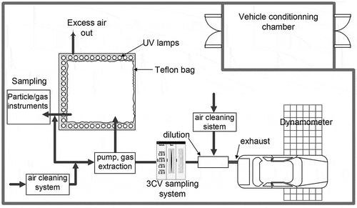
All experiments were performed at the Center for Vehicle Control and Certification (3CV) of Chile’s Ministry of Transport and Telecommunications in Maipú, Chile. The center is responsible for ensuring that all vehicles entering Chile comply with current Chilean law (Chilean Vehicular Emission Standards, 2012) and meets the specifications of the European Economic Community for measuring emissions of light-duty vehicles (EUR-Lex, 2007). Figure 1 shows a diagram of the 3CV emissions certification room, with the location of the dynamometer, vehicle, and the chamber. The test area is equipped with a AVL-Zöllner chassis dynamometer (Graz, Austria) and a Horiba constant-volume sampling system (model CVS 7200 T; Kyoto, Japan) that features three venturi pumps (30, 40, and 50 m³/min) that can operate singly or in combination, resulting in a flow range of 30–120 m³/min. A heat exchanger regulates the temperature of the exhaust gases within a controlled range (±11 °C). Other equipments include a Pierburg model FVT 458 stainless steel dilution tunnel (xx, xx), with gravimetric sampling system for particulate matter; an AVL Pierburg gas analyzing system for total hydrocarbons (THC) and nonmethane hydrocarbons (NMHC); a nondispersive infrared analyzer for carbon monoxide (CO) and carbon dioxide (CO₂); a chemiluminescence detector for nitrogen oxides (NO_x) and nitrogen dioxide (NO₂); and an AVL-Pierburg particle mass measurement instrument.

Figure 1. Diagram of the photochemical chamber and the 3CV measuring system.

Chamber system particle and gas continuous/semicontinuous monitoring

The chamber system was designed and developed at the Harvard T.H. Chan School of Public Health (HSPH) in Boston, Massachusetts, USA. A wooden enclosure was built adjacent to the light-duty vehicle test area’s shed. Over the wood surface, 90 light fixtures were mounted on the three inner sides of the walls of the enclosure (left, right, and rear) in two rows of 15 fixtures per row per enclosure side. A total of 180 ultraviolet lamps (UV-A, Q-LAB, Westlake, OH, USA) lamps were installed in the enclosure, with a total power 4.2 mW/cm² in the center of the chamber. This power is about 12% lower than the solar UV-A power at noon in a summer day in Santiago (4.8 mW/cm²). The total UV-A energy irradiated by the sun in a clear summer day is about 140 J/cm². The energy irradiated by the chamber in 8 hr is 120 J/cm²; thus, it is about 14% lower than the energy in a clear day in Santiago. The power distribution panel and the pumps system were installed on the outside of one of the corners of the enclosure. The walls of the chamber were constructed from 127-μm-thick fluorinated ethylene propylene (FEP) Teflon film (Welch Fluorocarbon Inc., Dover, NH, USA) to minimize wall reactions and adsorption of gas-phase compounds and to allow light transmission (Cocker et al., 2001). The Teflon film formed a cube shape of 2.4-m sides (13.82 m³) and was supported by a rigid structural framework mounted on the ceiling of the enclosure. The chamber filling and draining systems were subsequently installed and connected to the chamber. Clean air was used to flush the chamber for at least 14 hr before the start of all experiments. The clean air system, custom-built by HSPH, consisted of four stages in series: a particle prefilter, an IAQ GridBLOK (Doraville, GA, USA) to remove volatile organic compounds (VOCs), a Puracarb GridBLOK (Doraville, GA, USA) to remove acid gases and sulfur dioxide (SO₂), and an ultralow particulate air (ULPA) filter. The air sampling system, installed on the outer side of the rear wall of the wooden enclosure, was designed to operate at flow rates between 300 and 600 L/min. For example, during fill/drain cycle with vehicle primary emissions, the chamber was being filled with emissions for 46 min at a flow rate of 600 L/min, corresponding to two residence times or two complete chamber volume exchanges. At the same time, the chamber was being drained in dynamic mode with negligible variations in static pressure.

During the irradiation period, the instruments drained approximately 4.4 L/min of air to perform the different measurements. Consequently, a small pump was installed to fill the chamber at the same rate with clean air. This air was cleaned with a carbon activated filter and an ULPA filter. A pressure sensor was installed inside the chamber and one outside it in order to visually control variations in static pressure. The longest experiment lasted 540 min; thus, the maximum volume drained by the instruments was 2376 L, which corresponds to 17% of the chamber capacity. The measurements were not corrected for the dilution effect or loss to the walls of the chamber (Gordon et al., 2014b).

An array of monitors was employed to measure particles and gases upstream and downstream of the chamber during testing. To monitor the size distribution of particles between 15 and 700 nm, a scanning mobility particle sizer (SMPS) with an electrostatic classifier (model 3934; TSI, Shoreview, MN, USA) was used. Calibration of the SMPS was performed at Harvard University before being sent to the 3CV facility. A differential mobility analyzer (DMA; model 3081; TSI) based on Electrostatic Classifier 3080, running with Aerosol Instrument Manager software (version 9, TSI) and coupled with a water-based condensation particle counter (CPC; model 3785; TSI), was used to obtain continuous particle number information. Ozone formation inside the chamber during irradiation was measured by means of an ozone monitor (model 202; 2BTEC, Boulder, CO, USA). A portable CPC (model 3007; TSI) was used to measure particle count concentration. An NO/NO_y (with NO_y = NO+ NO₂ + other nitrogen oxides) monitor (model 42i; Thermo, xx, xx) was used to monitor continuous concentrations of NO/NO₂/NO_x before and during irradiation. Ozone and NO/NO_y monitors were provided by the Ministry of the Environment, and the monitors were calibrated using the same procedure used in the National Air Quality Network (SINCA), standard procedure. Chamber temperature and relative humidity (RH) were monitored by means of a temperature/relative humidity sensor (model HMD70Y; Vaisala, Helsinki, Finland).

Test vehicles, fuel blends, and driving cycle

Two vehicles were used for the tests. A 2012 model year flex-fueled Ford Focus 2.0 GDI and direct injection system. The vehicle was equipped with a three-way catalyst (TWC), and met the Tier 2, Bin 4 U.S. emission standard. The other vehicle was a Chevrolet Prisma 1.4 flex-fueled, engine type: Econoflex, indirect injection system. The vehicle was equipped with a three-way catalyst, and met the PROCONVE L-6 Brazil emission standard. The vehicles and the ethanol blends were manufactured in the United States and Brazil, respectively, in order to simulate the emission conditions in each place.

The U.S. car was tested with pure gasoline (E0) and three standard ethanol blends: 10% (E10), 85% (E85 summer; E85S), and 75% (E75 winter; E75W). The Brazilian car was tested with 22% ethanol (E22) and 100% ethanol (E100). The main physical and chemical properties of the fuel are given in Table 1.

Table 1. Gasoline fuel specifications.

Property	Method	E0	E10	E75	E85	E22	E100
RON	ASTM D2699	97.3	95.5	102.2	107.6	93.8
MON	ASTM D2700	88.2	85.7	88	89.2	82.3
Density (g/L)	ASTM D4052	742	745.5	773.3	787.6	735	809
Sulfur (wt.%)	ASTM D4294	0.0030	0.0029	0.0006	0.0006	0.06	0.0003
Reid VP (kPa)	ASTM D5191	62	68.6	82	45	51
Ethanol (vol.%)	ASTM D4815	0	10.3	74	82	22.2	93.3
Carbon (wt.%)	ASTM E191	86.29	82.74	59.66	57.60	76.68	48.7
Hydrogen(wt.%)	ASTM E191	13.43	13.46	13.54	13.14	13.69	12.3
Oxygen (wt.%)	ASTM D4815	<0.01	3.80	26.8	29.26	8.31	32.4
Lead (g/L)	ASTM D3237	n/d	n/d	n/d	n/d	n/d	n/d

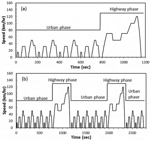
The tests had to be performed with a driving cycle that enabled at least two chamber volume exchanges, which corresponds to 46 min. The U.S. Federal Test Procedure (FTP) cycle lasts for 31.2 min, and in order to fill the chamber two times, the cycle had to be run two times, which corresponds to 62.4 min. The New European Driving Cycle (NEDC) lasts for 20 min, and to fill the chamber, the cycle had to be run two times and 6 more minutes, so the shortest cycle was selected. The tests were performed at room temperature (25 °C) using the NEDC (Bermúdez et al., 2015, and references therein). This test is divided in two parts: the urban driving cycle (UDC), which simulates the driving conditions in an urban area; and the extra urban driving cycle (EUDC), which simulates the driving conditions in a highway. Figure 2a shows the standard NEDC cycle. The complete cycle used with this study is shown in Figure 2b.

Figure 2. (a) New European Driving Cycle (NEDC). (b) The modified NEDC driving cycle with the additional time to complete 46 min as applied to all pilot tests and experiments.

Preconditioning of the vehicle and fuel was performed before each test. It consisted of a dynamometer run (one NEDC cycle) the previous day; subsequently the vehicle was left overnight in the laboratory in order to stabilize the temperature and humidity for at least 12 hr. One driver performed all the tests, which were executed over a period of 3 months.

Primary emission measurement

For each vehicle and fuel blend, primary emissions were measured using the 3CV standard dilute-bag approach described in Regulation No. 83 of the Economic Commission for Europe of the United Nations (EUR-Lex 2015). This procedure is used for regulated gaseous primary emissions of total hydrocarbons (THC), nonmethane hydrocarbons (NMHC), carbon monoxide (CO), nitrogen oxides (NO_x), and carbon dioxide (CO₂). In addition, a second set of measurements were performed in the chamber as described in the sections below. Both measurements are independent, and for each vehicle they were performed on different days.

An extraction probe was installed between the 3CV’s Constant Volume Sample–Critical Flow Venturi (CVS-CFV) blower and the laboratory ventilation particle filter. A 150 ft long, 2 in wide static dissipative duct hose was used to connect the extraction probe system with a vacuum pump. A vacuum pump (model R2303A; Oilless Regenerative Gast Blower, xx, xx) was connected to the air sampling system and was used to introduce the diluted vehicle exhaust into the photochemical chamber. This pump was used because of its clean operation and low noise and to reduce particle losses in the surfaces. The ambient temperature was 24 ± 2 °C, the relative humidity was 35 ± 6%, and the pressure was 962 ± 4 hPa.

The vehicle exhaust primary gases were monitored by the 3CV monitoring system for all the regulated gaseous emissions. The average concentrations of THC, CO, NO_x (NO), CO₂, methane (CH₄), and NMHC were reported. Emission factors were calculated from the mass of each of the gases and the mass of the fuel consumed with a procedure described in United Nations Economic Commission for Europe Regulation No. 83 (UN, 2011). Due to 3CV technical issues, the 3CV primary measurements were performed on different days from the chamber measurements. Only one fuel for each vehicle was performed on a given day. Ford Focus emissions for E10, E75W, E85S, and E0 were carried out on 28 July, 5 August, 12 August, and 20 October 2014, respectively. Chevrolet Prisma primary emissions for E22 and E100 were performed on 20 and 25 August 2014, respectively.

Pilot and duplicate experiments

For each ethanol blend in gasoline and each vehicle, a pilot test was performed to optimize the duration of irradiation needed to achieve the highest mass concentration of secondary aerosol formed. Subsequently, three more experiments were performed for each vehicle and blend type. The objective of the additional experiments was to collect particle samples for future toxicity studies (to be reported in a subsequent publication). The pilot test was used to determine the time needed to generate the maximum amount of secondary particulate material; thus, in the following experiments, collection of particles started after this maximum was reached. The pilot test and the subsequent experiments were also used to determine the variability of the emissions and formation of secondary gases or aerosol for each fuel blend. The variability in the secondary mass formation is described further below.

For each experiment, the vehicle was started on the dynamometer and primary emissions were introduced into the chamber. Approximately 46 min later, at t_i = 0 min, the vehicle engine was turned off, the flows through the chamber were stopped, the chamber was capped, the lamps were turned on, and the irradiation of primary emissions inside the photochemical reaction chamber began. Primary particles were being aged, and secondary organic aerosol was formed through the photochemical reactions of VOCs with the radicals formed in the chamber under the influence of the UV light. Particle and gas concentrations were monitored throughout the duration of a test, from the start of the vehicle on the dynamometer, through the chamber irradiation and to the secondary organic aerosol sampling. Subsequent experiments with a specific fuel blend were performed using the irradiation times established during pilot tests.

Results and discussion

Regulated primary emissions

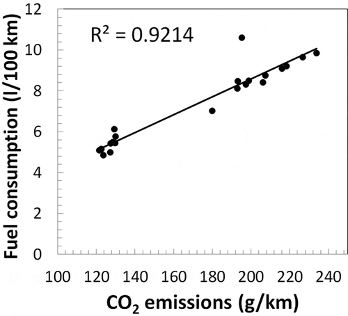
Regulated primary emissions were obtained using the 3CV standard monitoring technique as described before. Because the air flux and the distance traveled are known, it is possible to obtain the emission factors (in g/km). For each ethanol blend, only one test was performed, as detailed in Figure 2b. Because of variability in the test conditions, not all data are consistent. For example, for E0 during cold start, emissions of CO in the UDC phase (when the engine is cold) were lower than the EUDC phase (when the engine is hot). Emissions of NO_x for the Ford Focus during the UDC phase (hot or cold start) were always higher than the EUDC phase, but for the Chevrolet Prisma, it was the opposite. Data not consistent with previous work are shaded in Table 2. CO₂ emission is a good indicator for fuel consumption and can also be used to determine data that are not consistent. Figure 3 shows the consumption versus CO₂ emission from both vehicles, for all phases (UDC, EUDC) and start conditions (cold or hot). The correlation between these variables is very high (R² = 0.92). The points located far from the line are probably not consistent. CO data did not show good correlation with fuel consumption, most likely because the higher errors in the measurements.

Table 2. Exhaust EFs for both vehicles and all driving conditions as measured by 3CV sampling system.

		Driving condition								Fuel consumption
Vehicle	Fuel blend	Start	Phase	THC (g/km)	CO (g/km)	NOx (g/km)	CO2 (g/km)	CH4 (g/km)	NMHC (g/km)	L/100 km	km/L
U.S. car, Ford Focus 2.0 GDI	E0	Cold	UDC	0.203	0.275	0.027	226.6	0.057	0.150	9.667	10.3
			EUDC	0.066	0.515	0.009	128.4	0.015	0.052	5.494	18.2
		Hot	UDC	0.177	0.713	0.052	198.6	0.043	0.137	8.505	11.8
			EUDC	0.049	0.509	0.012	127.2	0.013	0.037	5.443	18.4
	E10	Cold	UDC	0.095	0.920	0.012	233.8	0.053	0.045	9.867	10.1
			EUDC	0.021	0.446	0.007	129.6	0.015	0.007	5.462	18.3
		Hot	UDC	0.110	0.817	0.037	207.4	0.046	0.068	8.756	11.4
			EUDC	0.023	0.449	0.020	129.5	0.016	0.008	5.460	18.3
	E75W	Cold	UDC	0.158	0.857	0.013	218.1	0.105	0.060	9.222	10.8
			EUDC	0.026	0.261	0.007	122.5	0.021	0.007	5.159	19.4
		Hot	UDC	0.098	0.542	0.022	197.2	0.066	0.036	8.318	12.0
			EUDC	0.026	0.296	0.010	122.5	0.022	0.005	5.160	19.4
	E85S	Cold	UDC	0.125	0.646	0.011	216.0	0.091	0.041	9.109	10.9
			EUDC	0.021	0.229	0.006	122.3	0.018	0.004	5.140	19.4
		Hot	UDC	0.083	0.486	0.027	192.9	0.059	0.028	8.130	12.3
			EUDC	0.020	0.215	0.009	121.5	0.017	0.004	5.110	19.6
Brazilian car Chevrolet Prisma 1.4 Flex	E22 Brazil	Cold	UDC	1.332	30.59	0.054	195.2	0.155	1.187	10.608	9.42
			EUDC	0.194	8.354	0.092	129.2	0.029	0.167	6.128	16.3
		Hot	UDC	0.247	5.509	0.055	193.0	0.040	0.210	8.488	11.8
			EUDC	0.113	4.851	0.108	129.8	0.020	0.094	5.777	17.3
	E100 Brazil	Cold	UDC	0.567	5.501	0.012	205.9	0.107	0.468	8.428	11.9
			EUDC	0.017	0.879	0.035	127.2	0.008	0.010	5.009	19.9
		Hot	UDC	0.048	0.297	0.029	179.8	0.023	0.026	7.024	14.2
			EUDC	0.014	0.796	0.037	123.5	0.007	0.007	4.859	20.6
U.S. emission standards^a					1.3	0.025
U.S. emission standards^b					0.63	0.019*
Brazil emission standards^c				0.30	2.0	0.12			0.05
Brazil emission standards^d				0.30	1.3	0.08			0.05

Note. Shaded numbers indicate measurements not consistent with previous work.

^aTier 2, Bin 4 tested with FTP-75 applied to the Ford Focus in this work.

^bThe most recent standard is Tier 3, Bin 30 tested with FTP-75.

^cPROCONVE L-5, tested with FTP-75 applied to the Chevrolet Prisma in this work.

^dThe most recent standard is PROCONVE L-6, tested with FTP-75.

*Refers to the sum of NMOG and NO_x.

Figure 3. Fuel consumption versus CO₂ emission from both vehicles, for all phases (UDC, EUDC) and start conditions (cold or hot).

The average emission factors (EFs) of the gases during cold and hot start are shown in Figure 4. The average and the standard deviation are calculated from the cold and hot start and the UDC and EUDC cycles. There are statistically significant decreases in THC for both vehicles, CO for the Chevrolet Prisma, NO_x for both vehicles, and NMHC for both vehicles. Table 2 shows emissions for the cold and hot start, for both cars according to the UDC or EUDC driving conditions. For comparison, the U.S. and Brazilian emission standards are also shown in Table 2. Both standards are tested with the FTP-75 driving cycle. The U.S. emission standard that applies to the Ford Focus used in this work is Bin 4, Tier 2 of the U.S. Environmental Protection Agency (EPA) regulations. The most recent standard is Bin 30, Tier 3, which is the most stringent level that the EPA believes it can be reasonable achieved (EPA, 2014). Bin 30, Tier 3 is a set of standards that have to be complied as a group, in which the sum of nonmethane organic gases (NMOG) and NO_x must be less than 30 mg/mile, CO must be less than 1.0 g/mile, HCHO less than 4 mg/mile, and PM less than 3 mg/mile. The limit in Table 2 and Figure 4 refers to NMOG + NO_x. The Brasilian emission standard refers to PROCONVE L-5, which applies to the Chevrolet Prisma used in this work. The most recent standard is PROCONVE L-6.

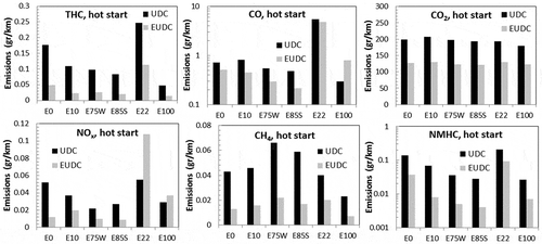
Figure 4. Average gaseous emissions for both cars and all gasoline blends as measured with the 3CV system. (a) Total hydrocarbons (THC). The standard deviation for the E22 bar is 0.58 g/km (b) carbon monoxide (CO), (c) carbon dioxide (CO₂), and (d) nitrogen oxides (NO_x). The standard deviation for the E22 bar is 0.027 g/km (e) methane (CH4) and (f) nonmethane hydrocarbons (NMHC). The standard deviation for the E22 bar is 0.52 g/km. The solid and dotted lines are the U.S. (Bin 4, Tier 2) and the Brazilian (PROCONVE L-6) emission standards, respectively.

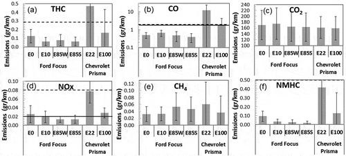
Table 2 shows that for all pollutants, the cold start has higher emissions than the hot start cycle, which is to be expected because the engine and catalyst are heating up. The emissions associated with the engine and the catalyst warm-up decline exponentially with time (Giannelli et al., 2014). CO emissions decrease 3% for the Ford Focus and 75% for the Chevrolet Prisma between cold and hot start. CO₂ emissions decrease 7% for the Ford Focus and 5% for the Chevrolet Prisma. The UDC also has higher emissions than the EUDC (except for NO_x for the Chevrolet Prisma). This behavior is common in all gasoline and diesel spark-ignition vehicles (Dardiotis et al., 2013; Hubbard et al., 2014; Karavalakis et al., 2014a, 2014b), because during acceleration, the air/fuel ratio is low (rich combustion) and there is less oxygen available for a complete combustion. This effect is seen in THC, where the UDC is 3–5 times larger than the EUDC for all blends for the Ford Focus (see Table 2). The EFs for the Ford Focus with an E85 blend are consistent with Suarez-Bertoa et al. (2015), which, in the UDC, obtained 0.273 g/km, versus 0.125 g/km in the present work. Dardiotis et al. (2015) tested two vehicles and obtained around 0.15 g/km for the UDC and about 0.01 g/km for EUDC, which is also consistent with this work. Hubbard et al. (2014) also saw a decrease with E30 and E40, but then an increase in THC emissions with E55 and E80. Karavalakis et al. (2014a) did not see a clear decrease in THC emissions with increasing ethanol content. It is clear that emissions have a strong dependence with vehicle characteristics (Karavalakis et al., 2014a).

The EFs for other regulated emissions (CO, NO_x, CO₂, and NMHC) are also consistent with previous studies (Clairotte et al., 2013; Dardiotis et al., 2015; Suarez-Bertoa et al., 2015). Emissions of CH₄ in this study are slightly larger than previous work: Clairotte et al. (2013) found 0.02 g/km for E85, versus 0.055 g/km in this work. CH₄ is the only regulated gas that increases its EFs with increasing ethanol content (see Figure 4). This increase may be a concern, considering that CH₄ has a large global warming potential of 25 eq g of CO₂ over 100 years. The mean emission factors (EFs) of the gases are presented in Figure 4 for both vehicles and all fuel blends. There is a tendency to decreased emissions with increasing ethanol content for all regulated emissions but CH₄. Figure 4 shows that the highest emissions are found with E0 (pure gasoline). This tendency has been realized before (Wallner and Frazee, 2010; Clairotte et al., 2013; Dardiotis et al., 2015; Timonen et al., 2017; Hubbard et al., 2014), but there is no comparison with E0 in some of these studies. The most probably reason for the decreased EFs is the higher amount of oxygen available in the fuel with higher ethanol content (Al-Hasan, 2003; Coordinating Research Council [CRC], 2009; Dardiotis et al., 2015). This oxygen improves the combustion process because the air/fuel ratio is modified, reducing incomplete combustion. Therefore, CO and THC are reduced. In this work, there is a small decrease in the CO emission from the Ford Focus, but a large decrease in the Chevolet Prisma. Hubbard et al. (2014b) found no trend in CO emissions, but Karavalakis et al. (2014) found a statistically significant reduction with higher ethanol blends. Figure 4 shows a decrease in NO_x emissions with higher ethanol blends for both vehicles. Turner et al. (2011) and Hubbard et al. (2014) also found a decreasing tendency in NO_x emissions when ethanol content in the fuel was increased; they argue that the lower flame temperature is responsible for this decrease. Emissions of NO_x, formaldehyde, and acetaldehyde are increased for E10 (Durbin et al., 2007), and there are larger increases with higher ethanol blends (Kousoulidou et al., 2008) compared with gasoline. However, in our work, NO_x emissions decrease with higher ethanol blends (see Figure 4). Similar decrease in NO_x was found by Timonen et al. (2017).

The tendency to decreasing EFs of CO, NO_x, THC, and NMHC with increasing ethanol content in the fuel is also observed when the driving phases are separated. The UDC hot start is plotted in Figure 5 for both vehicles (black bars). For THC, NO_x, and NHMH, during the UDC phase there is a decrease in emissions with increasing ethanol blends. During the EUDC phase (gray bars in Figure 5), there is a decrease in THC and NMHC. A similar trend between the UDC and EUDC is seen for cold start (not shown). There is also large difference in the EFs between the UDC and EUDC because of the engine and driving conditions, as has been found before (Wallner and Frazee, 2010; Clairotte et al., 2013; Dardiotis et al., 2015; Gordon et al., 2014a; Hubbard et al., 2014; Karavalakis et al., 2014a; Suarez-Bertoa et al., 2015). The average THC emissions decrease 75% from UDC to EUDC for the Ford Focus and decrease 55% for the Chevrolet Prisma. The average CO emissions decrease 43% from UDC to EUDC for the Ford Focus and decrease 3% for the Chevrolet Prisma. The tendency to decreasing EFs with higher ethanol content in the fuel can be seen for THC, CO, NO_x, and NMHC for the UDC and EUDC cycles (see Figure 5). CH₄ seems to be the only measured gas that increases EFs with ethanol content. Clairotte et al. (2013) found a change from 20 to 20.3 mg/km in the UDC between E5 and E85 for CH₄. In this work, CH₄ increased from about 45 to 60 mg/km between E10 and E85 (Figure 5) in the UDC phase.

Figure 5. Emissions during hot start for UDC and EUDC phases for the Ford Focus (E0, E10, E75W, and E85S) and Chevrolet Prisma (E22 and E100).

There are large differences in the EFs from the Chevrolet Prisma and the Ford Focus. This contrast is most likely due to the different technology of the cars and the formulation of the gasoline and ethanol. Table 1 shows the fuel properties. The Ford Focus was made in the United States, and the Chevrolet Prima was made in Brazil. The ethanol/gasoline mixtures for the two vehicles were imported from the United States and Brazil, respectively. For the Chevrolet Prisma, all gases decrease (see Figure 4) when the fuel is changed from E22 to E100. But the emissions for the E22 blend are very high to start. THC emissions for E22 are 0.47 g/km versus 0.062 g/km for the Ford Focus, or 0.102 g/km for a Euro 5–compliant vehicle with E85 blend (Suarez-Bertoa et al., 2015). The EFs for CO, NO_x, CH₄, and NMHC also are larger for the Chevrolet Prisma than the Ford Focus. NO_x is a precursor for O₃ in the atmosphere, so emission from ethanol blends might be the main reason for the high levels of O₃ observed in Brazilian cities (Corrêa et al., 2010). Fuel efficiency is reduced compared with gasoline when using ethanol blends (Durbin et al., 2007; Kousoulidou et al., 2008). In contrast, in this work, fuel efficiency remained the same for the Ford Focus at 15 km/L and increased slightly in the Chevrolet Prisma from 13.7 km/L with the E22 blend to 16.6 km/L with the E100.

Secondary gas formation

These experiments were performed in the chamber, and measurements were done with a different set of instruments than what was used for emission measurements. Filling of the chamber lasted 46 min at a flow rate of 600 L/min. At this time (t = 0), the UV lamps were turned on, and the instruments began measurements. The temperature in the chamber at the beginning of the experiments was 22–25 °C, and relative humidity was 30–35%. After the lights were turned on, temperature began to increase and RH began to decrease, as shown in Figure 6 for the E10 and E22 experiments. Similar values were obtained for the other ethanol blends. The maximum NO concentration inside the chamber was observed just before the lamps were turned on (t = 0). For t > 0, NO began reacting rapidly into NO₂ and its concentration decreased (Figure 6). For the U.S. vehicle and fuel blends, the lowest NO concentrations were observed for the U.S. E0. For the Chevrolet Prisma, NO concentration at the beginning of the experiment was much higher than the Ford Focus, and this difference is most likely related to the difference in car technology. A comparison of NO concentration measured by the 3CV system and initial NO concentration inside the chamber is shown in Table 3. There is a large variability in the NO measurements while the chamber is being filled and when the lamps are turned on, and the results are not the same. However, they have the same order of magnitude.

Table 3. NO concentration measured by the 3CV system and the average of the NO measurements inside the chamber at t_i = 0. Standard deviation is shown in parentheses.

		NO concentration
Vehicle	Fuel blend	3CV (ppb)	Chamber (ppb)
U.S. car, Ford Focus 2.0 GDI	E0	702	315 (89)
	E10	697	387 (73)
	E75W	460	636 (202)
	E85S	452	773 (31)
Brazilian car Chevrolet Prisma 1.4 Flex	E22	4780	2330 (665)
	E100	1380	934 (108)

Figure 6. NO, [NO_y − NO], and O₃ concentrations, temperature, and relative humidity inside the chamber (a) for the Ford Focus using E10 and (b) for the Chevrolet Prisma using the E22 ethanol blends versus irradiation time.

A review of the literature as published by Kousoulidou et al. (2008) in the European Topic Centre on Air and Climate Change reported that studies have shown very small changes in NO_x emissions with the addition of 10% ethanol (E10). Some studies have shown increases (Hsieh et al., 2002; Karavalakis et al., 2014a; Reuter et al., 1992), and other studies have shown a decrease (Dardiotis et al., 2015 Hubbard et al. 2014; Timonen et al., 2017). Larger changes have been reported for E20 blends, but not consistently. In this work, E100 fuel caused lower emission of NO_x than the E22 fuel in the Chevrolet Prisma. However, both fuels had very high NO_x emissions in the Brazilian car. It is not certain what caused this, whether this is typical, or whether lean fuel-air mixtures, improper oxygen sensor function, or improper function of the three-way catalyst may be contributing (Kousoulidou et al., 2008). The NO_x levels in the exhaust of the Chevrolet Prisma are of concern, because NO_x is a precursor of O₃ formation in the atmosphere.

O₃ is created in the photochemical chamber, as in the atmosphere, through reactions of NO₂ and hydrocarbons. O₃ is also formed through the reaction of atomic and molecular oxygen (O + O₂ → O₃). Atomic oxygen is produced through the photolysis of NO₂ (NO₂ + hν → NO + O(³P)) or through photodissociation of O₃ (O₃ + hν → O₂ + O(¹D)). In the first case, the energy needed is hν ≥ 3.18 eV (λ ≤ 398 nm); in the second case, the energy is hν ≥ 3.87 eV (λ ≤ 320 nm). The lamps have more energy in the first range, so the NO₂ dissociation is the dominant reaction in the chamber. The NO reacts very quickly with O₃ to regenerate NO₂, so for O₃ to accumulate in the chamber, there must be additional reaction pathways for the conversion of NO to NO₂ without consuming O₃ (Seinfeld and Pandis, 2006).

The initiation of these reactions in the chamber will include photolysis of different species present in the diluted exhaust, such as aldehydes (see eq 1 below). This is particularly important because photolysis of aldehydes can result in conversion of NO to NO₂ and also, ultimately, the production of ∙OH radical (Finlayson-Pitts and Pitts, 2000; Seinfeld and Pandis, 2006), through the following series of reactions:

(1)

The formyl radical (HCO∙) and alkyl radical (R∙) both quickly react with O₂ to form peroxy radicals; peroxy radicals react with NO to produce NO₂ and ∙OH (or ∙OR) radicals. ∙OH can then react with NO₂, SO₂, and hydrocarbons. The alkoxy radical (∙OR) can either react with O₂ to form a carbonyl compound and a peroxy radical or decompose to a smaller aldehyde and an alkyl radical; larger alkoxy radicals may also isomerize (Kroll and Seinfeld, 2005). Once the mechanism is initiated and radicals begin forming, the concentration of NO₂ in the chamber increases and the concentration of NO decreases, followed by accumulation of O₃ and secondary particulate mass.

Photolysis of O₃ by ultraviolet light (280 < ν < 310) nm produces an oxygen atom in a highly excited state O(¹D), which reacts with water to produce ∙OH radicals. This will occur to some extent in the photochemical chamber, where the lamps have some energy in that spectral region. Over time, the concentration of NO_x continues to decrease as NO₂ reacts with ∙OH to form nitric acid (HNO₃). HNO₃ reacts with ammonia (NH₃) to form ammonium nitrate particles (NH₄NO₃) or is lost to the walls of the chamber. These reactions consume ∙OH radical and can be considered terminating reactions. When reacting with organic molecules, ∙OH will generally abstract a hydrogen atom from the molecule, creating a radical that quickly reacts with O₂ to form an alkyl or acylperoxy radical. These reactions regenerate radicals, so that photochemical oxidation continues.

The NO, [NO_y − NO], and O₃ concentrations inside the chamber are shown in Figure 5 for both cars. The instrument measures NO_y (with NO_y = NO + NO₂ + other nitrogen oxides) and NO and reports as NO₂ the difference of [NO_y − NO]. Most of this difference is likely to be NO₂, but in the chamber the concentrations of other NO_y species, such as HNO₃, may be high enough to contribute. In Figure 6, it can be clearly seen that there is conversion from NO to [NO_y − NO] because as the second increases, the first decreases. Also, significant O₃ accumulation occurs after [NO_y − NO] > NO. However, the concentration of [NO_y − NO] relative to O₃ is much higher in the Ford Focus than in the Chevrolet Prisma. For the Ford Focus with the E10 blend, the maximum O₃ concentration is about 40% higher than the [NO_y − NO] maximum concentration (for the E0 blend it is 17% lower, for E75W the maximums are similar, for E85S it is 40% lower). For the Chevrolet Prisma with the E22 blend, the maximum O₃ concentration is 75% lower (for the E100 blend, O₃ is 80% lower).

A possible explanation for the lower relative amount of O₃ in the Chevrolet Prisma is that this vehicle generates much higher amounts of NO; thus, when NO₂ starts forming O₃, there is still a lot of NO in the chamber that consumes O₃ (NO + O₃ → NO₂ + O₂). Figure 6 shows that when NO₂ concentration reaches the maximum, the amount of NO in the Chevrolet Prisma is about 150 ppb, whereas in the Ford Focus, the amount of NO is about 35 ppb. The decrease in O₃ after it reaches the maximum is partly due to conversion into particles and dilution because the instruments remove air continuously.

The maximum concentration of NO and [NO_y − NO] seems to be dependent on the amount of ethanol on the gasoline and the type of engine. Figure 7 shows the average maximum concentration of NO and [NO_y − NO] measured inside the chamber for all tests; the error bars show the standard deviation calculated from all tests. Although there is a large variability in some points, in the Ford Focus, there is a tendency to generate more NO with higher ethanol content. This is consistent with the work of Kousoulidou et al. (2008), which found higher NO with higher ethanol blends. For the Chevrolet Prisma, lower formation of NO and [NO_y − NO] is observed for E100. Another difference between blends and car types is the time that it takes to reach the maximum concentration for [NO_y − NO] and O₃ (see Table 4). The shortest time to reach the maximum formation of [NO_y − NO] occurs for the Ford Focus with the E0 blend (45 min). As the fraction of ethanol increases, the time increases, and reaching 110 min for the E85S blend. Similar trend occurs for O₃ in the Ford Focus. For the Chevrolet Prisma, the time to reach the [NO_y − NO] maximum is longer for E100 than for the E22 blend.

Table 4. Maximum concentrations inside the chamber for NO, secondary NO₂ (NO_x − NO), and O₃ and mass and time to reach the maximum for all blends.

		Maximum (SD)				Time to max. (minutes)
Vehicle	Ethanol content (%)	NO (ppb)	NO2 (ppb)	O3 (ppb)	Mass (μg/m^3)	NO2	O3	Mass
Ford Focus	0 (E0)	315 (89)	98 (15)	62 (6)	792 (56)	45	123	145
	10 (E10)	387 (73)	102 (31)	103 (6)	605 (86)	80	150	180
	75 (E75W)	636 (202)	150 (59)	96 (5)	428 (30)	90	164	190
	85 (E85S)	773 (31)	154 (16)	99 (2)	407 (32)	110	229	195
Chevrolet Prisma	22 (E22)	2330 (665)	1180 (359)	125 (61)	891 (253)	130	164	195
	100 (E100)	934 (108)	508 (79)	92 (6)	505 (69)	145	255	255

Note. Standard deviations are in parentheses.

Figure 7. Maximum concentrations measured in the chamber for all ethanol blends for (a) NO, Ford Focus; (b) NO₂, Ford Focus; (c) NO, Chevrolet Prisma; (d) NO₂, Chevrolet Prisma.

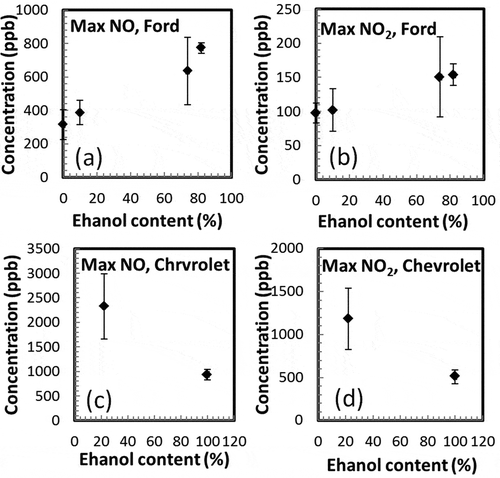
An increase in the NO, [NO_y − NO], and O₃ concentrations, but not the mass (Table 2), can be seen for the Ford Focus as the ethanol content increase. In contrast, for the Chevrolet Prisma, lower concentrations are found for all gases and mass for the blend with higher ethanol (E100).

Secondary particle formation

PM mass was not measure directly using a standard instrument; rather, an effective mass concentration was obtained from the SMPS assuming spherical particles with a density of 1.2 g/cm³. To obtain the ratio of secondary to primary PM concentration, the mass was estimated using the SMPS before the lights were turned on and when the mass concentration reached the maximum. The ratio was calculated after subtracting the primary mass concentration. The average of the four tests for each blend is shown in Figure 8. The error bars were calculated from the standard deviation of the data. There are several conditions that add uncertainty to these numbers. Secondary particle concentration is affected by the wall losses and the removal of air by the instruments monitoring the chamber (Gordon et al., 2014a); however, data have not been corrected for these effects because they could not be quantified. The SMPS efficiency is also very sensitive to particle shape, which can change as particles grow, condense into each other or onto existing particles. The SMPS used in this study measured particles larger than 14 nm and had low efficiency for particles lower than ~25 nm. RH can also affect SOA formation. Seinfeld et al. (2001) found an increase in SOA formation with high RH. In the chamber, RH decreased from 35% to about 15% after 50 min (see Figure 6), and similar values were obtained for other ethanol blends. Thus, SOA formation was not affected by RH.

Figure 8. PM concentrations measured with the SMPS in the chamber before (primary) and after (secondary) irradiation. The numbers above the columns show the ratio of secondary to primary PM concentration, but for blends larger than ~10 the ratio is overestimated.

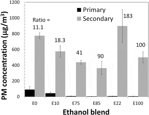
It can be seen in Figure 8 that for both cars there is a decrease in primary mass concentration when the ethanol content in fuel increases. Maricq et al. (2012) and Timonen (2017) also observed a similar decrease. The concentration of secondary PM in the chamber also decreases as the ethanol content increases. This is similar the results from Timonen et al. (2017), which saw a decrease in secondary particle formation. Secondary to primary PM ratios are also shown in Figure 8 and increased with increased ethanol content in fuel the American car, but decreased in the Brazilian car. For E0 and E10, the secondary to primary PM ratios are similar to those reported in previous studies (Gordon et al., 2014a; Suarez-Bertoa et al., 2015; Timonen et al., 2017). But for E75W, E85S, and for the Chevrolet Prisma, secondary to primary PM ratios are much higher than in previous studies, which could be due to an underestimation of the primary mass by the SMPS with these blends. Dutcher et al. (2011) using a nano-DMA found a decrease in the concentration of primary particles larger than 10 nm with higher ethanol blends. But for particles smaller than 10 nm, they found a sharp increase in the number, with higher ethanol blends exceeding the number of particles measured at E0. The instrument used in this study did not measure particles below 14 nm and had lower efficiency for particles below ~25 nm. Thus, the primary to secondary PM ratios for higher ethanol blends are overestimated because the SMPS could not measure the lower part of the size spectrum. Although secondary ratios for higher ethanol blends are overestimated, the measurement of secondary PM is not overestimated because most of the mass is in higher size range where the SMPS measures correctly.

For all blends, secondary PM formation occurs with the initial nucleation of ultrafine particles, which then coagulate and grow with condensation of material into particle phase. For all blends, the maximum of the mass concentration is reached after the maximum in O₃.

For exhausts from each vehicle, the irradiation time required to reach the maximum secondary mass concentration increased with the ethanol content of the fuel; the U.S. E0-diluted exhaust achieved its maximum secondary particle mass concentration after 145 min, whereas the U.S. E85S reached its maximum concentration at t_i = 195 min. The Brazilian E22 required 195 min whereas the BR E100 required 255 min of irradiation to reach the maximum. The time required to reach the maximum mass concentration does not seem to be related to the initial amount of NO, because in the Ford Focus NO increases with ethanol blends and in the Chevrolet Prisma it decreases.

The highest secondary mass concentration was observed for the E22 blend in the Chevrolet Prisma (see Figure 8). For the Ford Focus, the maximum mass concentration is not directly related to the amount of initial NO (which is a precursor for particle mass) because it increases with higher ethanol blends (see Figure 7). This is an indication that other precursors dominate secondary mass generation. For the Chevrolet Prisma, the maximum mass concentration may be directly related to the amount of initial NO because it decreases with higher ethanol blends. Decreasing primary mass concentration is consistent with several previous studies (Dutcher et al. 2011; Mulawa et al., 1997) that demonstrate that increasing ethanol fraction decreases particle mass as well as other species such as carbon monoxide and many hydrocarbon species, including benzene, toluene, and butadiene. However, some other species may increase, such as unburned ethanol, methane, total hydrocarbons, some aldehyde species, and ethylene (Clairotte et al., 2013; Durbin et al., 2007; Graham et al., 2008; Suarez-Bertoa et al., 2015; Timonen et al., 2017). Dutcher et al. (2011) saw an increase in Ca⁺ and Zn⁺. Timonen et al. (2017) found decreasing secondary PM concentration for 10%, 85%, and 100% ethanol blends.

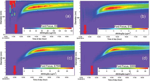
Figure 9 shows the evolution of the particle size distribution for the U.S. vehicle test (Ford Focus) with four different ethanol blends as monitored with the SMPS. After about 2 hr of irradiation, a maximum in the size distribution of ~300 nm is reached for E0. For E10, E75W, and E85S, the time needed to reach the maximum increases to about 3, 3.5, and 3.6 hr (see Table 4).

Figure 9. Secondary particle size distribution inside the chamber versus irradiation time as measured with the SMPS for the Ford Focus with (a) E0 blend, (b) E10 blend, (c) E75W blend, and (d) E85S blend. The arrow in each panel indicates when the lights are turned on.

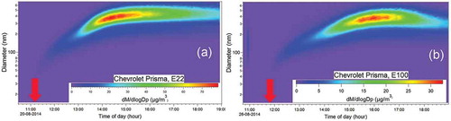
Figure 10 shows the evolution of the exhaust from the Chevrolet Prisma fueled with E22 and E100. As with the Ford Focus, as irradiation time increases, particles grow larger. For E22, the maximum in the particle size distribution is reached after approximately 3 hr of irradiation (Table 4), and for E100, the maximum is reached about 5 hr later. The decrease in PM after it reaches the maximum is partly due to losses into the wall and dilution because the instruments remove air continuously.

Figure 10. Secondary particle size distribution inside the chamber versus irradiation time as measured with the SMPS for the Chevrolet Prisma with (a) E22 blend and (b) E100 blend. The arrow in each panel indicates when the lights are turned on.

Figures 9 and 10 show that the time that it takes to reach the maximum size concentration increases with ethanol content, but also that the shape of the size distribution also changes with ethanol content. During the first hour, the particle size distribution has a maximum around 200 nm for E0 and 150 nm for E10, but only reaches 100 nm for E75W and E85S. For the Chevrolet Prisma, for both blends, the number of particles also reaches a maximum of about 100 nm during the first hour and 200 nm after ~2.5 hr. The following hours, the distribution moves to the right, i.e., the maximum of the size distribution increases and there are more large particles reaching 400 nm after 7 hr. It appears that with ethanol fractions greater than ~10%, particles have a slower growth. The lower growth speed may be related to the lower emission of aromatic compounds (benzene, toluene, ethylbenzene, xylenes), which are considered the most important PM precursors among anthropogenic hydrocarbons (Gordon et al., 2014a; Suarez-Bertoa et al., 2015; Timonen et al., 2017).

Conclusion

Two flex-fueled vehicles using different ethanol blends in gasoline were used to study primary and secondary gas and particle concentrations. One vehicle (Ford Focus) and its fuels were made in the United States, whereas the other vehicle (Chevrolet Prisma) and its fuels were made in Brazil. Primary emissions of THC, CO, CO₂, and NMHC for both cars decreased as the fraction of ethanol in gasoline increased, which is consistent with previous studies. NO_x was also seen to decrease with increasing ethanol content for the Ford Focus and the Chevrolet Prisma. However, emissions of HC, CO, and NO_x from the Brazilian car were substantially higher than the American car, showing that emissions are strongly dependent on car technology and formulation of the gasoline and ethanol. Fuel efficiency remained approximately the same for both vehicles.

In the Brazilian car, formation of secondary NO₂ and O₃ was lower for the E100 than the E22 blend. In the American car, a small increasing trend was seen with increasing ethanol for NO₂ and O₃. The maximum concentration of NO₂ relative to O₃ is much higher in the American car than in the Brazilian car, although no clear explanation was found for this difference. Secondary particle formation in the chamber was observed for both vehicles and the mass concentration decreased as the fraction of ethanol in fuel increased, consistent with previous studies. Secondary to primary PM ratio of 11 was found for E0 and 18 for E10, but for higher ethanol blends, the ratio is overestimated, as discussed previously. For both vehicles, the time required to form secondary PM is longer for higher ethanol blends, which may be related to lower emission of aromatic compounds. These results indicate that using higher ethanol blends may have a positive impact on air quality.

Acknowledgment

Technical support was provided by Mr. Raúl Albarrán and Marcelo Cornejo at the Center for Control and Certification of Vehicles.

Additional information

Funding

Financial support for this project was provided by the Inter-American Development Bank (Ms. Gloria Visconti) and Fondo Nacional de Desarrollo Científico y Tecnológico (Fondecyt) project no. 1151117.

Notes on contributors

E. Gramsch

Ernesto Gramsch is a research professor at the Physics Department of the University of Santiago de Chile, Santiago, Chile.

V. Papapostolou

Vasileios Papapostolou is an Air Quality Specialist for Science & Technology Advancement at the South Coast Air Quality Management District, Diamond Bar, CA, USA.

P. Oyola

Pedro Oyola and Gianni López are directors at Mario Molina Center for Strategic Studies of Energy and Environment, Santiago, Chile.

S. Ferguson

Felipe Reyes, Yeanice Vásquez and Marcela Castillo are research associates at Mario Molina Center for Strategic Studies of Energy and Environment, Santiago, Chile.

M. Wolfson

Alfonso Cádiz is the Director of the Center for Control and Certification of Vehicles, Santiago, Chile.

J. Lawrence

Alfonso Cádiz is the Director of the Center for Control and Certification of Vehicles, Santiago, Chile.

P. Koutrakis

Steve Ferguson, Mike Wolfson and Joy Lawrence are research professors at Harvard T. H. Chan School of Public Health, Harvard University, Boston, MA, USA.

Petros Koutrakis is the Head of the Exposure, Epidemiology and Risk Program and the Director of the EPA/Harvard University Center for Ambient Particle Health Effects.

References

- Al-Hasan, M. 2003. Effect of ethanol–unleaded gasoline blends on engine performance and exhaust emission. Energy Convers. Manage. 44:1547–61. doi: 10.1016/S0196-8904(02)00166-8.
- Bahreini, R., A.M. Middlebrook, J.A. De Gouw, C. Warneke, M. Trainer, C.A. Brock, H. Stark, S.S. Brown, W.P. Dube, J.B. Gilman, K. Hall, J.S. Holloway, W.C. Kuster, A.E. Perring, A.S.H. Prévôt, J.P. Schwarz, J.R. Spackman, S. Szidat, N.L. Wagner, R.J. Weber, P. Zotter, and D.D. Parrish. 2012. Gasoline emissions dominate over diesel in formation of secondary organic aerosol mass. Geophys. Res. Lett. 39:L06805. doi: 10.1029/2011GL050718.
- Bermúdez, V., J.M. Luján, S. Ruiz, D. Campos, and W.G. Linares. 2015. New European Driving Cycle assessment by means of particle size distributions in a light-duty diesel engine fuelled with different fuel formulations. Fuel 140:649–59. doi: 10.1016/j.fuel.2014.10.016.
- Borbon, A., J.B. Gilman, W.C. Kuster, N. Grand, S. Chevaillier, A. Colomb, C. Dolgorouky, V. Gros, M. Lopez, R. Sarda-Esteve, J. Holloway, J. Stutz, H. Petetin, S. McKeen, M. Beekmann, C. Warneke, D.D. Parrish, and J.A. de Gouw. 2013, “Emission ratios of anthropogenic volatile organic compounds in northern mid-latitude megacities: Observations versus emission inventories in Los Angeles and Paris”, J. GeoPhys. Res.: Atmospheres. 118:2041–57, doi:10.1002/jgrd.50059.
- Böhm, G.M., Saldiva, P.H.N., Massad, E., Pasqualucci, A.A.G. Muñoz, D.R., Gouveia, M.A., Cardoso, L.M.N., Caldeira, M.P.R. and Silva, R. 1988. Health effects of hydrate etanol used as automobile fuel. Proc. VIIIth Int. Symp. Alcohol Fules. 1201–5.
- Budisulistiorini, S.H., M.R. Canagaratna, P.L. Croteau, W.J. Marth, K. Baumann, E.S. Edgerton, S.L. Shaw, E.M. Knipping, D.R. Worsnop, J.T. Jayne, A. Gold, and J.D. Surratt. 2013. Real-time continuous characterization of secondary organic aerosol derived from isoprene epoxydiols in Downtown Atlanta, Georgia, using the aerodyne aerosol chemical speciation monitor. Environ. Sci. Technol. 47:5686–94. doi: 10.1021/es400023n.
- Chilean Vehicular Emissions Standards. 2012. Regulation on light duty vehicle emissions. Library of the Congress Web site. http://www.leychile.cl/Navegar?idNorma=11031 (accessed May 2016).
- Clairotte, M., T.W. Adam, A.A. Zardini, U. Manfredi, G. Martini, A. Krasenbrink, A. Vicet, E. Tournié, and C. Astorga. 2013. Effects of low temperature on the cold start gaseous emissions from light duty vehicles fuelled by ethanol-blended gasoline. Appl. Energy 102:44–54. doi: 10.1016/j.apenergy.2012.08.010.
- Cocker, D.R., III, R.C. Flagan, and J.H. Seinfeld. 2001. State-of-the-art chamber facility for studying atmospheric aerosol chemistry. Environ. Sci. Technol. 35:2594–2601. doi: 10.1021/es0019169.
- Cook, R., S. Phillips, M. Houyoux, P. Dolwick, R. Mason, C. Yanca, M. Zawacki, K. Davidson, H. Michaels, C. Harvey, J. Somers, and D. Luecken. 2011. Air quality impacts of increased use of ethanol under the United States’ Energy Independence and Security Act. Atmos. Environ. 45:7714–24. doi: 10.1016/j.atmosenv.2010.08.043.
- Corrêa, S.M., G. Arbilla, E.M. Martins, S.L. Quitério, C.D.S. Guimarães, and L.V. Gatti. 2010. Five years of formaldehyde and acetaldehyde monitoring in the Rio de Janeiro downtown area–Brazil. Atmos. Environ. 44:2302–8. doi: 10.1016/j.atmosenv.2010.03.043.
- Corrêa, S.M., E.M. Martins, and G. Arbilla. 2003. Formaldehyde and acetaldehyde in a high traffic street of Rio de Janeiro, Brazil. Atmos. Environ. 37:23–9. doi: 10.1016/S1352-2310(02)00805-1.
- Coordinating Research Council. 2009. Effects of Vapor Pressure, Oxygen Content, and Temperature on CO Exhaust Emissions. Report no. E-74b, 123, May. https://crcao.org/news/Mid%20Level%20Ethanol%20program/index.html (accessed December 2017)..
- Dardiotis, C., G. Fontaras, A. Marotta, G. Martini, and U. Manfredi. 2015. Emissions of modern light duty ethanol flex-fuel vehicles over different operating and environmental conditions. Fuel 140:531–40. doi: 10.1016/j.fuel.2014.09.085.
- Dardiotis, C., G. Martini, A. Marotta, and U. Manfredi. 2013. Low-temperature cold-start gaseous emissions of late technology passenger cars. Appl. Energy 111:468–78. doi: 10.1016/j.apenergy.2013.04.093.
- De Andrade, J.B., M.V. De Andrade, and H.L.C. Pinheiro. 1998. Atmospheric levels of formaldehyde and acetaldehyde and their relationship with the vehicular fleet composition in Salvador, Bahia, Brazil. J. Braz. Chem. Soc. 9:219–23. doi: 10.1590/S0103-50531998000300004.
- De Gouw, J.A., C.A. Brock, E.L. Atlas, T. S. Bates, F.C. Fehsenfeld, P.D. Goldan, J. S. Holloway, W.C. Kuster, B.M. Lerner, B.M. Matthew, A.M. Middlebrook, T.B. Onasch, R.E. Peltier, P. K. Quinn, C.J. Senff, A. Stohl, A.P. Sullivan, M. Trainer, C. Warneke, R.J. Weber, and E.J. Williams. 2008. Sources of particulate matter in the northeastern United States in summer: 1. Direct emissions and secondary formation of organic matter in urban Plumes. J. Geophys. Res. 113 doi: 10.1029/2007JD009243.
- DeServes, C. 2005. Emissions from flexible fuel vehicles with different etanol blends. Report no 5509; 2005. ISSN: 1103-0240. Haninge, Sweden: AVL MTC. http://korridor.se/aryan/acadiane/e85/Etanolrapport.pdf (accessed December 2017)).
- Dockery, D.W., and C.A. Pope. 1994. Acute respiratory effects of particulate air pollution. Annu. Rev. Public Health 15:107–32. doi: 10.1146/annurev.pu.15.050194.000543.
- Dockery, D.W., C.A. Pope, X.P. Xu, J.D. Spengler, J.H. Ware, M.E. Fay, B.G. Ferris, and F.E. Speizer. 1993. An association between air pollution and mortality in 6 United States cities. N. Engl. J. Med. 329:1753–59. doi: 10.1056/NEJM199312093292401.
- Durbin, T.D., J.W. Miller, T. Younglove, T. Huai, and K. Cocker. 2007. Effects of fuel ethanol content and volatility on regulated and unregulated exhaust emissions for the latest technology gasoline vehicles. Environ. Sci. Technol. 41:4059–64. doi: 10.1021/es061776o.
- Dutcher, D., M.R. Stolzenburg, S.L. Thompson, J.M. Medrano, D.S. Gross, D.B. Kittelson, and P.H. McMurry. 2011. Emissions from ethanol-gasoline blends: A single particle perspective. Atmosphere 2:182–200. doi: 10.3390/atmos2020182.
- EUR-Lex. 2007. Regulation (EC) No. 715/2007 of the European Parliament and of the Council of 20 June 2007 on type approval of motor vehicles with respect to emissions from light passenger and commercial vehicles (Euro 5 and Euro 6) and on access to vehicle repair and maintenance information. http://eur-lex.europa.eu/legal-content/EN/ALL/?uri=CELEX%3A32007R0715 (accessed February 2017).
- EUR-Lex. 2015. Regulation No 83 of the Economic Commission for Europe of the United Nations (UNECE) — Uniform provisions concerning the approval of vehicles with regard to the emission of pollutants according to engine fuel requirements [2015/1038]. http://data.europa.eu/eli/reg/2015/83/oj (accessed December 2017).
- European Commission. On the promotion of the use of energy from renewable sources and amending and subsequently repealing Directives 2001/77/EC and 2003/30/EC. Directive 2009/28/EC., Official Journal of the European Union L140/16 2009. Brussels, Belgium: European Union.
- Feilberg, A., T. Ohura, T. Nielsen, M.W.B. Poulsen, T. Amagai. 2002. Occurrence and photostability of 3-nitrobenzanthrone associated with atmospheric particles. Atmos. Env. 36:3591–600.
- Finlayson-Pitts, B., and J.N. Pitts. 2000. Chemistry of the Upper and Lower Atmosphere: Theory, Experiments, and Applications. San Diego, CA: Academic Press.
- Giannelli, R., R. Stubleski, and A. Saunders. 2014. Semi-empirical analysis of cold start emissions. SAE Int. J. Fuels Lubr. 7:591–9. doi: 10.4271/2014-01-1619.
- Gordon, T.D., A.A. Presto, A.A. May, N.T. Nguyen, E.M. Lipsky, N.M. Donahue, A. Gutierrez, M. Zhang, C. Maddox, P. Rieger, S. Chattopadhyay, H. Maldonado, M. M. Maricq, and A. L. Robinson. 2014a. Secondary organic aerosol formation exceeds primary particulate matter emissions for light-duty gasoline vehicles. Atmos. Chem. Phys. 14:4661–78. doi: 10.5194/acp-14-4661-2014.
- Gordon, T.D., A.A. Presto, N.T. Nguyen, W.H. Robertson, K. Na, K.N. Sahay, M. Zhang, C. Maddox, P. Rieger, S. Chattopadhyay, H. Maldonado, M.M. Maricq, and A.L. Robinson. 2014b. Secondary organic aerosol production from diesel vehicle exhaust: Impact of aftertreatment, fuel chemistry and driving cycle. Atmos. Chem. Phys. 14:4643–59. doi: 10.5194/acp-14-4643-2014.
- Graham, L., S. Belisle, and C. Baas. 2008. Emissions from light duty gasoline vehicles operating on low blend ethanol gasoline and E85. Atmos. Environ. 42:4498–4516. doi: 10.1016/j.atmosenv.2008.01.061.
- Gramsch, E., F. Reyes, Y. Vásquez, P. Oyola, and M.A. Rubio. 2016. Prevalence of freshly generated particles during pollution episodes in Santiago de Chile. Aerosol Air Qual. Res. 16:2172–85. doi: 10.4209/aaqr.2015.12.0691.
- Hsieh, W., R. Chen, T. Wu, and T. Lin. 2002. Engine performance and pollutant emission of an SI engine using ethanol-gasoline blended fuels. Atmos. Environ. 36:403–10. doi: 10.1016/S1352-2310(01)00508-8.
- Hubbard, C.P., J.E. Anderson, and T.J. Wallington. 2014. Ethanol and air quality: Influence of fuel ethanol content on emissions and fuel economy of flexible fuel vehicles. Environ. Sci. Technol. 48:861–7. doi: 10.1021/es404041v.
- Ilabaca, M., I. Olaeta, E. Campos, J. Villaire, M.M. Tellez-Rojo, and I. Romieu. 1999. Association between levels of fine particulate and emergency visits for pneumonia and other respiratory illnesses among children in Santiago, Chile. J. Air Waste Manage. Assoc. 49:154–63. doi: 10.1080/10473289.1999.10463879.
- Karavalakis, G., D. Short, R.L. Russell, H. Jung, K.C. Johnson, A. Asa-Awuku, and T.D. Durbin. 2014a. Assessing the impacts of ethanol and isobutanol on gaseous and particulate emissions from flexible fuel vehicles. Environ. Sci. Technology 48:14016–24. doi: 10.1021/es5034316.
- Karavalakis, G., D. Short, D. Vu, M. Villela, A. Asa-Awuku, and T.D. Durbin. 2014b. Evaluating the regulated emissions, air toxics, ultrafine particles, and black carbon from SI-PFI and SI-DI vehicles operating on different ethanol and iso-butanol blends. Fuel 128:410–21. doi: 10.1016/j.fuel.2014.03.016.
- Kent Hoekman, S. 2009. Biofuels in the U.S.—Challenges and opportunities. Renew. Energy 34:14–22. doi: 10.1016/j.renene.2008.04.030.
- Kleindienst, T.E., Corse, E.W., Li. W., McIver, C.D., Conver, T.S., Edney, E.O., Driscoll, D.J., Speer, R.E., Weathers, W.S., and Tejada, S.B. 2002. Secondary organic aerosol formation from the irradiation of simulated automobile exhaust. J. Air Waste Manage. Assoc. 52:259–72. doi: 10.1080/10473289.2002.10470782
- Kousoulidou, M., G. Fontaras, G. Mellios, and L. Ntziachristos. 2008. Effect of Biodiesel and Bioethanol on Exhaust Emissions. Technical Paper 2008/5. European Topic Centre on Air and Climate Change. .
- Kroll, J., and J.H. Seinfeld. 2005. Representation of secondary organic aerosol laboratory chamber data for the interpretation of mechanisms of particle growth. Environ. Sci. Technol. 39:4159–65. doi: 10.1021/es048292h.
- Lambe, A.T., A.T. Ahern, L.R. Williams, J.G. Slowik, J.P.S. Wong, J. P. D. Abbatt, W.H. Brune, N.L. Ng, J.P. Wright, D.R. Croasdale, D.R. Worsnop, P. Davidovits, and T.B. Onasch. 2011. Characterization of aerosol photooxidation flow reactors: Heterogeneous oxidation, secondary organic aerosol formation and cloud condensation nuclei activity measurements. Atmos. Meas. Tech. 4:445–461. doi: 10.5194/amt-4-445-2011.
- Lambe, A.T., P.S. Chhabra, T.B. Onasch, W.H. Brune, J.F. Hunter, J. H. Kroll, M.J. Cummings, J.F. Brogan, Y. Parmar, D.R. Worsnop, C.E. Kolb, and P. Davidovits. 2015. Effect of oxidant concentration, exposure time, and seed particles on secondary organic aerosol chemical composition and yield. Atmos. Chem. Phys. 15:3063–75. doi: 10.5194/acp-15-3063-2015.
- Lim, H.-J., and B.J. Turpin. 2002.Origins of primary and secondary organic aerosol in Atlanta: Results of time-resolved measurements during the Atlanta supersite experiment. Environ Sci. Technol. 36:4489–96.
- Maricq, M., J.J. Szente, and K. Jahr. 2012. The impact of ethanol fuel blends on PM emissions from a light-duty GDI vehicle. Aerosol Sci. Technol. 46:576–83. doi: 10.1080/02786826.2011.648780.
- Moreno, F., Gramsch, E., Oyola, P., Rubio., M.A. 2010. Modification in the soil and traffic-related sources of particle matter between 1998 and 2007 in Santiago de Chile. J. Air Waste Manage. Assoc. 60:1410–21. doi: 10.3155/1047-3289.60.12.1410
- Massad, E., C. Saldiva, L. Nunes-Cardoso, R. Da Silva, P. Saldiva, G. Böhm. 1985. Acute toxicity of gasoline and ethanol automobile engine exhaust gases. Toxicology Letters. 26:187–92.
- Mulawa, P.A., S.H. Cadle, K. Knapp, R. Zweidinger, R. Snow, R. Lucas, and J. Goldbach. 1997. Effect of ambient temperature and E-10 fuel on primary exhaust particulate matter emissions from light-duty vehicles. Environ. Sci. Technol. 31:1302–7. doi: 10.1021/es960514r.
- Ng, N.L., M.R. Canagaratna, Q. Zhang, J.L. Jimenez, J. Tian, I.M. Ulbrich, J.H. Kroll, K.S. Docherty, P.S. Chhabra, R. Bahreini, S.M. Murphy, J.H. Seinfeld, L. Hildebrandt, N.M. Ng, S.C. Herndon, A. Trimborn, M.R. Canagaratna, P.L. Croteau, T.B. Onasch, D. Sueper, D.R. Worsnop, Q. Zhang, Y.L. Sun, and J.T. Jayne. 2011. An Aerosol Chemical Speciation Monitor (ACSM) for routine monitoringof the composition and mass concentrations of ambient aerosol. Aerosol Sci. Technol. 45:780–94. doi: 10.1080/02786826.2011.560211.
- Nguyen, H.T.-H., Takenaka, N., Bandow, H., Maeda, Y., de Oliva, S.T., Botelho, M. M.f.,Tavares, T.M., 2001. “Atmospheric alcohols and aldehydes concentrations measured in Osaka, Japan, and in Sao Paulo, Brazil”, Atmos. Environ. 35:3075–83.
- Nikolaou, K., Masclet, P., and Mouvier, G., 1984. Sources and reactivity of polycyclic aromatic hydrocarbons in the atmosphere: A critical review. The Science of the Total Environment. 32:103–31.
- Papapostolou, V., J.E. Lawrence, E.A. Diaz, J.M. Wolfson, S.T. Ferguson, M.S. Long, J.J. Godleski, and P. Koutrakis. 2011. Laboratory evaluation of a prototype photochemical chamber designed to investigate the health effects of fresh and aged vehicular exhaust emissions. Inhal. Toxicol. 23:495–505. doi: 10.3109/08958378.2011.587034.
- Renewable Fuels Association. 2015. Going Global: 2105 Ethanol Industry Outlook. https://ethanolrfa.3cdn.net/c5088b8e8e6b427bb3_cwm626ws2.pdf (accessed February 2017).
- Reuter, R., J. Benson, V. Burns, J. Gorse, A. Hochhauser, W. Koehl, L. Painter, B. Rippon, and J. Rutherford. 1992. Effects of Oxygenated Fuels and RVP on Automotive Emissions—Auto/Oil Air Quality Improvement Program. SAE Technical Paper 920326. Warrendale, PA, USA: SAE International. doi: 10.4271/920326
- Ryan, L., F. Convery, S. Ferreira. 2006. Stimulating the use of biofuels in the European Union: Implications for climate change policy. Energy Policy. 34:3184–94. doi: 10.1016/j.enpol.2005.06.010.
- Sato, K., A. Takami, Y. Kato, T. Seta, Y. Fujitani, T. Hikida, A. Shimono, and T. Imamura. 2012. AMS and LC/MS analyses of SOA from the photooxidation of benzene and 1,3,5-trimethylbenzene in the presence of NOx: Effects of chemical structure on SOA aging. Atmos. Chem. Phys. 12:4667–82. doi: 10.5194/acp-12-4667-2012.
- Seinfeld, J.H., G.B. Erdakos, W.E. Asher, and J.F. Pankow. 2001. Modeling the formation of secondary organic aerosol (SOA). 2. The predicted effects of relative humidity on aerosol formation in the α-pinene-, β-pinene-, sabinene-, Δ3-carene-, and cyclohexene-ozone systems. Environ. Sci. Technol. 35:1806–17.
- Seinfeld, J.H., and S.N. Pandis. 2006. Atmospheric Chemistry and Physics—From Air Pollution to Climate Change, 2nd ed. Hoboken, NJ: John Wiley & Sons.
- SINCA. 2017. Ministry of the Environment National Air Quality Network. http://sinca.mma.gob.cl/ (accessed February 2017).
- Suarez-Bertoa, R., A.A. Zardini, S.M. Platt, S. Hellebust, S.M. Pieber, I. El Haddad, B. Temime-Roussel, U. Baltensperger, N. Marchand, A.S.H. Prévôt, and C. Astorga. 2015. Primary emissions and secondary organic aerosol formation from the exhaust of a flex-fuel (ethanol) vehicle. Atmos. Environ. 117:200–11. doi: 10.1016/j.atmosenv.2015.07.006.
- Sun, Y., Z. Wang, H. Dong, T. Yang, J. Li, X. Pan, P. Chen, and J.T. Jayne. 2012. Characterization of summer organic and inorganic aerosols in Beijing, China with an aerosol chemical speciation monitor. Atmos. Environ. 51:250–9. doi: 10.1016/j.atmosenv.2012.01.013.
- Timonen, H., P. Karjalainen, E. Saukko, S. Saarikoski, P. Aakko-Saksa, P. Simonen, T. Murtonen, M. Dal Maso, H. Kuuluvainen, E. Ahlberg, B. Svenningsson, J. Pagels, W.H. Brune, J. Keskinen, D.R. Worsnop, R. Hillamo, and T. Rönkkö. 2017. Influence of fuel ethanol content on primary emissions and secondary aerosol formation potential for a modern flex-fuel gasoline vehicle. Atmos Chem. Phys. 17:5311–29. doi: 10.5194/acp-17-5311-2017.
- Tkacik, D.S., A.T. Lambe, S. Jathar, X. Li, A.A. Presto, Y. Zhao, D. Blake, S. Meinardi, J.T. Jayne, P.L. Croteau, and A.L. Robinson. 2014. Secondary organic aerosol formation from in-use motor vehicle emissions using a potential aerosol mass reactor. Environ. Sci. Technol. 48:11235–42. doi: 10.1021/es502239v.
- Turner, D., H. Xu, R.F. Cracknell, V. Natarajan, and X. Chen. 2011. Combustion performance of bio-ethanol at various blend ratios in a gasoline direct injection engine. Fuel 90:1999–2006. doi: 10.1016/j.fuel.2010.12.025.
- United Nations. 2011. United Nations Economic Commission for Europe, Regulation 83, Revision 4 Uniform Provisions Concerning the Approval of Vehicles with Regards to the Emission of Pollutants According to Engine Fuel Requirements.
- U.S. Environment Protection Agency. 2014. Control of Air Pollution from Motor Vehicles: Tier 3 Motor Vehicle Emission and Fuel Standards; Final Rule, April 28, Vol. 78, No. 81. https://www.epa.gov/regulations-emissions-vehicles-and-engines/final-rule-control-air-pollution-motor-vehicles-tier-3 ( accessed xxx).
- US Energy Information Administration. 2015. Annual energy outlook 2015 with projections to 2040. https://www.eia.gov/outlooks/aeo/pdf/0383(2015).pdf. (Accessed December 2017).
- Volkamer, R., J.L. Jimenez, F.S. Martini, K. Dzepina, Q. Zhang, D. Salcedo, L. T. Molina, D.R. Worsnop, and M.J. Molina. 2006. Secondary organic aerosol formation from anthropogenic air pollution: Rapid and higher than expected. Geophys. Res. Lett. 33:L17811. doi: 10.1029/2006GL026899.
- Wallner, T., and R. Frazee. 2010. Study of Regulated and Non-Regulated Emissions from Combustion of Gasoline, Alcohol Fuels and Their Blends in a DI-SI Engine. SAE Technical Paper 2010-01-1571. Warrendale, PA, USA: SAE International.
- Wang, M., C. Saricks, and D. Santini. 1999. Effects of Fuel Ethanol Use on Fuel-Cycle Energy and Greenhouse Gas Emissions. Lemont, IL: Argonne National Laboratory. http://www.anl.gov/energy-systems/publication/effects-fuel-ethanol-use-fuel-cycle-energy-and-greenhouse-gas-emissions (accessed February 2017).
- Zhang, Q., J.L. Jimenez, M.R. Canagaratna, J.D. Allan, H. Coe, I. Ulbrich, M.R. Alfarra, A. Takami, A.M. Middlebrook, Y.L. Sun, K. Dzepina, E. Dunlea, K. Docherty, P.F. De-Carlo, D. Salcedo, T. Onasch, J.T. Jayne, T. Miyoshi, A. Shimono, S. Hatakeyama, N. Takegawa, Y. Kondo, J. Schneider, F. Drewnick, S. Borrmann, S. Weimer, K. Demerjian, P. Williams, K. Bower, R. Bahreini, L. Cottrell, R.J. Griffin, J. Rautiainen, J.Y. Sun, Y.M. Zhang, and D.R. Worsnop. 2007. Ubiquity and dominance of oxygenated species in organic aerosols in anthropogenically-influenced Northern Hemisphere mid-latitudes. Geophys Res. Lett. 34:L13801. doi: 10.1029/2007GL029979.