Evaluating potential human health risks from modeled inhalation exposures to volatile organic compounds emitted from oil and gas operations

ABSTRACT

Some states and localities restrict siting of new oil and gas (O&G) wells relative to public areas. Colorado includes a 500-foot exception zone for building units, but it is unclear if that sufficiently protects public health from air emissions from O&G operations. To support reviews of setback requirements, this research examines potential health risks from volatile organic compounds (VOCs) released during O&G operations.

We used stochastic dispersion modeling with published emissions for 47 VOCs (collected on-site during tracer experiments) to estimate outdoor air concentrations within 2,000 feet of hypothetical individual O&G facilities in Colorado. We estimated distributions of incremental acute, subchronic, and chronic inhalation non-cancer hazard quotients (HQs) and hazard indices (HIs), and inhalation lifetime cancer risks for benzene, by coupling modeled concentrations with microenvironmental penetration factors, human-activity diaries, and health-criteria levels.

Estimated exposures to most VOCs were below health criteria at 500–2,000 feet. HQs were < 1 for 43 VOCs at 500 feet from facilities, with lowest values for chronic exposures during O&G production. Hazard estimates were highest for acute exposures during O&G development, with maximum acute HQs and HIs > 1 at most distances from facilities, particularly for exposures to benzene, 2- and 3-ethyltoluene, and toluene, and for hematological, neurotoxicity, and respiratory effects. Maximum acute HQs and HIs were > 10 for highest-exposed individuals 500 feet from eight of nine modeled facilities during O&G development (and 2,000 feet from one facility during O&G flowback); hematologic toxicity associated with benzene exposure was the critical toxic effect. Estimated cancer risks from benzene exposure were < 1.0 × 10⁻⁵ at 500 feet and beyond.

Implications: Our stochastic use of emissions data from O&G facilities, along with activity-pattern exposure modeling, provides new information on potential public-health impacts due to emissions from O&G operations. The results will help in evaluating the adequacy of O&G setback distances. For an assessment of human-health risks from exposures to air emissions near individual O&G sites, we have utilized a unique dataset of tracer-derived emissions of VOCs detected at such sites in two regions of intense oil-and-gas development in Colorado. We have coupled these emission stochastically with local meteorological data and population and time-activity data to estimate the potential for acute, subchronic, and chronic exposures above health-criteria levels due to air emissions near individual sites. These results, along with other pertinent health and exposure data, can be used to inform setback distances to protect public health.

Introduction

Colorado’s rapidly growing population, in parallel with increased oil-and-gas (O&G) extraction in Colorado’s Northern Front Range (NFR) and Garfield County (GC), has led to increasing numbers of people living and working in close proximity to O&G wells (McKenzie et al. 2016; McMullin et al. 2018).

The upper part of Colorado’s NFR, in the Wattenberg Field area of the Denver-Julesburg (D-J) sediment basin (see Figure 1), saw population grow by 19% in 2008–2017 (CODOLA 2019). It is a particularly intense region of O&G development (COGCC 2007) where O&G production grew by over 300% in that period, almost entirely in Weld and Larimer counties (COGCC 2019).

Figure 1. The major oil-and-gas-producing regions of Colorado and the locations of meteorological stations used for dispersion and exposure assessment. Interstate highways are also indicated.

In western Colorado, in GC and neighboring Rio Blanco and Mesa counties, population grew by 8% in 2008–2017 (CODOLA 2019). In those areas, O&G development of the Uinta-Piceance (U-P) basin (see Figure 1) has continued. O&G production declined 10% in 2008–2017 (peaking around 2012 at 26% over 2008 levels), though production in 2018 was higher relative to 2017, particularly in Mesa County with 48% growth (COGCC 2019).

In these Colorado regions, residential areas are often found within hundreds of feet (ft) of O&G wells. In 1992–2013, Colorado’s Exception Zone Setback Distance was 350 ft (107 meters [m]) from the centre of new wells and production facilities to a building unit, and in 2013 the Colorado Oil and Gas Conservation Commission (COGCC) Rule #604 updated it to 500 ft (152 m). Analyses of residential locations in 2010 indicated 131,000 Coloradans lived within 400 m (1,312 ft) of a confirmed active well, with 255,000 people within 800 m (2,625 ft) (Czolowski et al. 2017). A more focused analysis of 2012 populations within 500 ft of active wells indicated 14,488 people in the D-J Basin live in such areas (up from 6,801 people in 2000) and 177 people in the more sparsely populated U-P basin live in that proximity (up from 72 people in 2000) (McKenzie et al. 2016). Because of continued population increases in these areas, a growing public-health concern has developed about the potential for inhalation health risks to people living near existing and future wells.

A number of studies have correlated proximity to O&G development with adverse health outcomes at different stages of life (Casey et al. 2016; Hill 2018; McKenzie et al. 2014, 2017; Rabinowitz et al. 2015; Stacy et al. 2015; Tustin et al. 2017; Whitworth, Marshall, and Symanski 2017, 2018). However, Haley et al. (2016) reviewed setback distances in Texas, Pennsylvania, West Virginia, Ohio, and Maryland, and they found the setbacks were not determined from peer-reviewed data analysis but were based on compromise between government agencies, the regulated community, environmental and citizen groups, and landowners. A limited number of studies which have provided more robust recommendations on safe setbacks (Maryland School of Public Health 2014) are based on limited data on epidemiology and air-quality monitoring.

Numerous studies in the literature analyzed ambient monitoring data near wells and locations of intense O&G development. Several studies analyzed airborne volatile organic compounds (VOCs) measured near O&G-production facilities in the Wattenberg Field (Gilman et al. 2013; McMullin et al. 2018; Thompson, Hueber, and Helmig 2014) as well as in the vicinity of tank batteries and O&G-processing and disposal sites in the NFR (Halliday et al. 2016; McKenzie et al. 2018). Swarthout et al. (2013) and Colborn et al. (2014) respectively measured VOC signals in the Wattenberg Field area and in areas of O&G development in western Colorado.

Studies have used such monitoring data to estimate exposures for people living near O&G operations. Long, Briggs, and Bamgbose (2019) did so for areas in Pennsylvania. For Coloradans within 0.5 miles of active wells in 2008, McKenzie et al. (2012) used measurements along well-pad perimeters to make conclusions about incremental exposures to O&G-related hydrocarbon emissions: higher-end subchronic exposures could be slightly above health-criteria levels, while all other subchronic and chronic exposures were below non-cancer criteria levels for individual critical-effect groups and chemicals, and cancer risks from individual chemicals were < 1 × 10⁻⁵. Similarly, McMullin et al. (2018) used existing Colorado monitoring data, generally at hundreds-to-thousands of feet from well sites, to extrapolate that incremental acute and chronic exposures to O&G-related VOC emissions were below non-cancer criteria levels, and cancer risks were ≤ 1x10⁻⁵, at ≥ 500 ft from wells (beyond the current setback distance).

Most of the monitoring data used by McKenzie et al. (2012) and McMullin et al. (2018) were not at the hourly resolution ideal for acute-exposure analyses, and neither study used measured, source-attributable emission rates, nor human-activity patterns or other microenvironmental analyses, to more comprehensively examine spatiotemporal dispersion and exposure patterns. Studies or regulators conducting dispersion modeling of O&G operations often use limited, generic, and outdated emission factors (Small et al. 2014). This is particularly important because emissions from O&G activities can vary greatly in time and by phase of O&G activity (Adgate, Goldstein, and McKenzie 2014; Allen 2016; Brantley, Thoma, and Eisele 2015; CSU, 2016a, 2016b; McMullin et al. 2018; Thompson et al. 2017; Hecobian et al. 2019). This is especially pertinent to acute chemical exposures, which at high levels can be associated with headaches, nosebleeds, fatigue, dizziness, etc., depending on the chemical, intensity of exposure, and sensitivity of the individual.

In general, at sites using current well-development technologies, there remains a relative lack of studies utilizing measured emission rates to examine the direct impact from well-development and -production activities and corresponding patterns of acute human exposures. The relatively weak links between emissions and exposure must be strengthened to design and implement effective strategies to protect public health (Small et al. 2014). New studies are needed to help fill critical data gaps in O&G-related air-quality and exposure issues across geographies and communities, including using human-activity patterns to assess exposures that are epidemiologically meaningful (Shonkoff, Hays, and Finkel 2014).

In this article, we detail an assessment of human-health inhalation risks in Colorado regions of intense O&G activity (the NFR and GC), which helps to fill these data gaps. We utilized on-site VOC-emission rates derived by Colorado State University (CSU) during tracer studies, where during periods in 2013–2016 they measured 46 VOCs plus ethane (which we refer to as “47 VOCs” for convenience) at individual sites of O&G well development and production in the NFR and GC (CSU 2016a, 2016b; Hecobian et al. 2019). Their measurements indicated high intra-hour emission variability (by several orders of magnitude), occurring with no pattern. We used stochastic methods to model those variable emissions on an hourly basis, along with several sets of local hourly meteorological data and human-activity patterns in a variety of microenvironments (MEs). The modeled well sites are hypothetical because CSU measured the emissions at a variety of sites and times, and because the meteorological data we used in the modeling were not from the same sites and times. We stratified estimated risks by region, number of wells per well pad, O&G phase of activity (drilling, hydraulic fracturing (“fracking”), flowback, and production), VOC (and group of VOCs with similar critical effects), and duration of exposure (acute, subchronic, and chronic). The risk calculations, at distances ≤ 2,000 ft from the well pads, utilize health criteria issued by federal and state regulatory agencies, for non-cancer assessments of all VOCs and cancer-risk assessments for benzene. All exposures and risks are incremental (due only to each hypothetical well site being modeled) and do not consider aggregated exposure from background sources or other well sites. The risk estimates are only due to the 47 modeled VOCs and do not consider other compounds known to be emitted by O&G activities, and we do not account for synergistic health effects that may result from multi-chemical exposure.

While our chief concern is the highest simulated exposures (to determine if any exposure scenarios have the potential for adverse health impacts), we also characterize the distributions of potential non-cancer hazards across all modeled individuals at locations of higher average air concentrations.

The methodology developed and applied in this assessment can be applied to other O&G well operations which employ fracking and related processes. Ideally, local measurements of VOC emissions would be available, but the measurements used in this study could be used in a screening approach while still incorporating local meteorological, topographical, and human-activity data to inform determinations of safe setback distances.

Methods and approach

In this section, we describe the methods and approach of our assessment. We discuss the uncertainties of some of these methods, and the sensitivity of the assessment to those methods, in the Uncertainties and Limitations section as well as in Supplementary Sections F and G.

Air-dispersion modeling

Model selection

We used the American Meteorological Society/U.S. Environmental Protection Agency (EPA) Regulatory Model (AERMOD version 16216r) (EPA 2018a). AERMOD’s formulation represents the state of the science, with similarity-theory-based boundary-layer calculations. The steady-state Gaussian assumption is appropriate over the distances under consideration in this study, which are 150–2,000 ft (46–610 m). Near-source air concentrations are largely determined from emission source strength and meteorological conditions.

Emission characterization

We used field measurements made by CSU (2016a, 2016b; Hecobian et al. 2019) in close proximity to individual O&G-well sites in GC and the NFR, for the 47 VOCs shown in Figure 2. They gathered measurements during O&G drilling (only at GC sites) as well as fracking and flowback (at GC and NFR sites), which are development activities, as well as during O&G production (only at NFR sites). There were ≥ 12 sampling events per O&G phase, and each event had at least one unique canister sample measurement. In their documentation, CSU does not provide the exact locations of the sampled sites. They derived emission rates using the tracer-ratio method (TRM; Lamb et al. 1995). Wells et al. (2015) analyzed of the accuracy of the TRM using several controlled-release experiments, finding a mean bias of +22.6% and a precision (relative standard deviation) of ±16.7%. The CSU studies did not examine any chemicals beyond these 47 VOCs and methane.

Figure 2. Emission rates utilized in this assessment. The values shown are the superset of rates from all sites and operations, and they are 1-hour-average rates derived from the 3-minute-average rates from CSU (2016a, 2016b; Hecobian et al. 2019). The bottom and top of the boxes are the 25th and 75th percentiles, respectively; the line inside the box represents the median; the bottom and top whiskers are the 5th and 95th percentiles, respectively; and the asterisks are outliers beyond the 5th and 95th percentiles.

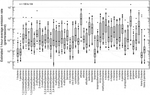
Measured 3-minute-average emission rates for each VOC were highly variable. From the 3-minute-average rates, we derived 1-hour-average rates appropriate for dispersion modeling (1 hour is also the shortest time scale for acute health/toxicity information). We provide in Supplementary Section A further details on the characterization of emission variability and derivation of 1-hour-average emission rates. In Figure 2, for each VOC we show the superset of derived 1-hour-average emission rates (across all modeled sites and O&G activities).

To model emissions in AERMOD, we assumed multi-well development sites (which are increasingly common) would be larger than single-well sites. We modeled three source configurations for O&G development to reasonably represent current and near-future practices, based on professional judgement and recent O&G permits submitted to COGCC: a 1-acre site (for 1 well), a 3-acre site (for 8 wells in the NFR and 16 wells in GC), and a 5-acre site (for 32 wells). These acreages correspond to 0.4, 1.2, and 2 hectares. We modeled O&G well production using a 1-acre site (without consideration of the number of wells; production emissions were not well correlated with the number of producing wells). We characterized each site as a volume source, implying emissions come equally from all parts of the well pad, and with no chemical transformations during the short travel times/distances of interest (2,000 ft).

Meteorology

Meteorological data, provided by CDPHE, were representative of conditions in our two study areas (and generally representative of the regions where the CSU experiments occurred), and they included terrain-induced flows, mountain/valley wind systems, local-scale weather systems, and continental-scale weather effects. We show in Figure 1, and describe further in Supplementary Section B (including processing details and wind roses), the selected representative meteorological stations: a GC valley site (Rifle, Colorado), a ridge-top site 24 kilometres (km) north of GC (“BarD” site), an NFR site influenced by ridge flows (Anheuser-Busch site near Fort Collins, Colorado), and an NFR site influenced by mountain/valley flows (Ft. St. Vrain site near Platteville, Colorado). Terrain was generally flat within the immediate vicinity (500-m radius) of each station.

Receptors

We placed air-concentration receptors in a polar grid extending to 2,000 ft from the centre of a modeled well pad, at relatively regular distance intervals starting at 300 ft (91 m) from the development pad – at 100-ft (30-m) intervals to 1,000 ft (305 m), and then at 200-ft (61-m) intervals to 2,000 ft. We also included a 350-ft distance, and for modeling of well production we included receptors at 150 ft and 250 ft (76 m). Some distances (e.g., 350, 500, and 1,000 ft) correspond to setback distances from the centre of well or production facilities as listed under the COGCC Rule #600 Series Safety Regulations.

Monte Carlo simulations for O&G development

Since O&G well development typically lasts days to months, the focus was on short-term concentrations, which can vary drastically depending on meteorology and activities at the well. Dispersion models are designed primarily for sources with known emission rates or well-defined temporal patterns. For sources like O&G facilities emiting with substantial irregularity, the acute health risk can be exaggerated when applying an air-dispersion model to the improbable coincidence of the highest emission rate with worst-case meteorological conditions. To provide information on the probability of these events, the results are best expressed as a probability distribution simulated by randomizing the emission rate, O&G-activity duration, and meteorological conditions through application of the Monte Carlo method. The Monte Carlo approach is widely used in addressing problems associated with emissions from irregularly emitting sources, as it provides more realistic estimates of health risk (Li, Huang, and Zou 2008; Lonati and Zanoni 2013). Monte Carlo has been used to determine protective zones for intermittent irregular sources (Balter and Faminskaya 2016). For irregularly varying power-plant emissions, the Electric Power Research Institute sponsored the development of a Monte Carlo tool, EMVAP (Paine et al. 2014), useful in assessing compliance with National Ambient Air Quality Standards (NAAQS; Guerra 2014). The approach has been endorsed by the State of Washington’s Department of Ecology (Bowman and Dhammapala 2011) for use in compliance with the 1-hour NAAQS for nitrogen dioxide.

To determine the concentration distributions of VOCs emitted by development activities, we used the Monte Carlo approach illustrated in Figure 3, whereby we randomized key inputs: meteorology, emissions, and O&G-activity duration. Per-well activity durations ranged 3–7 days for drilling, 1–5 days for fracking, and 1–30 days for flowback (with typically longer flowback durations at GC sites) (see Supplementary Section A, Table A-1). These durations were developed from information provided by COGCC and O&G operators/supervisors in GC and the NFR. The output of the Monte Carlo approach provides a representative distribution of possible VOC concentrations (EPA 1994).

Figure 3. Monte Carlo simulation logic for estimating the concentration distribution of volatile organic compounds (VOCs) emitted by oil-and-gas well-development activities.

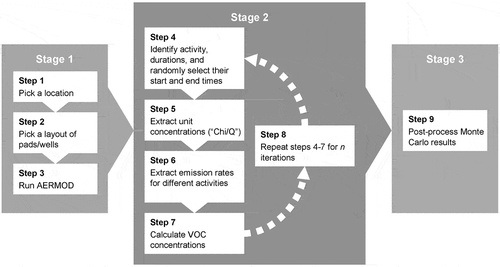
In Stage 1, for each of the four sites and three well-pad sizes, we ran AERMOD using unit-emission rates (1 gram/second/pad) for the full meteorological period, retaining all hourly results and producing concentrations per unit emissions (“Chi/Q”). In Stage 2, for a given O&G development activity, we randomly selected a duration per well for the activity (from the ranges and probabilities shown in Supplementary Section A, Table A-1) and a time when the activity occurred. Then, for each VOC, we randomly selected an emission rate from available measurements and multiplied it by the Chi/Q values, resulting in a period of hourly modeled VOC concentrations (per well) based on the emission rate and meteorological variability. Each scenario developed in this way is termed an “iteration.” This process was repeated 2,000 times for each well-pad size, meteorological dataset, O&G activity, and VOC. We identified 2,000 iterations was sufficient for result stability by running 10,000 simulations for VOCs with large emission-rate variations, examining maxima and standard deviations in the maximum concentrations. We assumed with all other O&G activities and VOCs that additional iterations would not noticeably alter the distributions of results, as they have less variability. Note: because the NFR is so large, neither meteorological station’s data set fully characterizes the geographical region; as a result, for the NFR we randomly selected the iterations from the model outputs using the Anheuser-Busch or Ft. St. Vrain meteorological data, producing a blended single set of model results broadly representative of the NFR.

In Stage 3, we post-processed the Monte Carlo results by summarizing their statistical distributions. The goal was to constrain the amount of data passed to the exposure assessment of O&G-development emissions, utilizing only the receptors with the highest concentrations and only summary statistics of the Monte Carlo results at those receptors. First, we identified the maximum 1-hour-average concentration from each iteration, at each receptor for a specific O&G site (GC valley and ridge-top sites; NFR blended site), activity, and VOC. Second, we calculated the means from each set of maxima (the mean-maximum values, representing the expected maximum concentrations). Third, from among all the receptors at a given distance from the well pad, we identified the receptor with the highest mean-maximum concentration, for a specific O&G site, activity, and VOC. Fourth and finally, for each highest-mean-maximum receptor identified (one per receptor distance), we characterized the distribution of the concentrations from across the iterations for use in exposure assessment.

O&G production

Since O&G production typically lasts decades, the focus was long-term air concentrations. We used AERMOD to generate full years of hourly Chi/Q values for receptors at each O&G site, from which we calculated the annual-average values. As with O&G development, we sought to constrain the data passed to the exposure and risk assessments by focusing on the higher-concentration locations. We identified the year with the highest annual average for each site, and then we identified the receptor at each distance with the highest annual average. These receptors (one per receptor distance) with the highest annual-average Chi/Q represent the locations with the highest long-term concentrations, based on prevailing meteorological conditions. For each receptor identified, we later used the Chi/Q values directly in exposure and risk assessment, where we randomly combined the hourly Chi/Q values with the VOC emissions rates, creating many random hourly combinations of emission rate and meteorological conditions.

Comparison with monitored data

We cannot compare directly to CSU’s canister measurements (2016a, 2016b; Hecobian et al. 2019) because we were not attempting to simulate the conditions and other specifications under which they took the measurements. We considered comparison to samples collected in other O&G studies. Halliday et al. (2016) collected samples of ambient VOCs, but they mostly focused on a regional scale and captured other VOC sources such as on-road mobile sources, biogenic emissions, other O&G-processing facilities, and industrial sources. However, we considered one site in that study appropriate for comparison: the PAO site was located 9 km southeast of Platteville, Colorado (in the NFR), in a fairly isolated, primarily rural location surrounded by agricultural and grazing lands but with active wells in close proximity and collection tanks 500 m to the southwest. The maximum benzene concentration reported at this location, using observations at 1-second time resolution, was 29.3 parts per billion (ppb). Our Monte Carlo dispersion simulations during well-development activities using the Anheuser-Busch meteorological data found an expected-maximum 1-hour concentration of 87.3 ppb at the much closer distance of 152 m, decreasing to 13.8 ppb at 610 m. While these data cannot be directly compared given the different source mix and distances, they indicate peak benzene concentrations are likely to be in the range of 10–100 ppb in the nearby vicinity under reasonable worst-case conditions. Other studies such as Thompson, Hueber, and Helmig (2014) only measured concentrations from samples in close proximity to producing wells and lack information on meteorology or emission rate needed to make a model-to-monitor comparison. McMullin et al. (2018) argued the need for more extensive and detailed air and exposure monitoring to improve the body of real-world data.

Human-exposure modeling

Model selection

We conducted inhalation-exposure modeling using the U.S. EPA Air Pollutants Exposure (APEX) Model, a stochastic, ME model used by EPA for assessments of criteria air pollutants (e.g., assessments for NAAQS; see, for example, EPA 2018b) and other airborne-chemical scenarios (EPA 2017). It generates time series of estimated inhalation exposure across a population by combining data on demographics, human activity, pollutant-ME interactions, and ambient pollutant concentrations.

Characterization of ambient air concentrations

We developed APEX runs whose results could be combined with the modeled air concentrations to obtain exposure estimates for a wide variety of scenarios. As illustrated in Figure 4, each run utilized unit ambient-air concentrations, resulting in time series of exposure concentrations per unit outdoor VOC air concentration, specific to the O&G site as well as chemical-penetration group and age group (discussed later). We multiplied the exposure time series by time series of air concentrations constructed from the Monte Carlo dispersion iterations.

Figure 4. Flow diagram illustrating the steps in exposure assessment. Notes: O&G = oil and gas; VOC = volatile organic compound; AERMOD = American Meteorological Society/U.S. Environmental Protection Agency Regulatory Model; APEX = U.S. Environmental Protection Agency Air Pollutants Exposure Model; max = maximum.

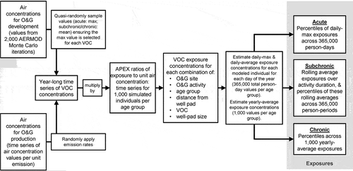
For estimating exposure concentrations during O&G-development activities, we used outputs from the Monte Carlo dispersion iterations of O&G development to construct year-long time series of outdoor VOC concentrations. Each time series was specific to a VOC, O&G site, and development activity. For estimating acute exposure above criteria levels, each hour utilized the absolute-maximum 1-hour outdoor concentration from a randomly selected dispersion iteration (acute effects are likely to begin shortly after exposure but may persist for 24 hours or longer; we based our 1-hour time frame on the durations used to calculate acute health-criteria values). For estimating the potential for subchronic and chronic exposures above criteria levels, each hour utilized the mean outdoor concentration from a random iteration. Concentrations for all VOCs for a given hour originated from the same CSU sampling experiment, enabling evaluation of simultaneous chemical exposures.

For estimating exposure concentrations during O&G production, we generated year-long time series of outdoor VOC concentrations by multiplying hourly production emission rates (55 values per VOC available from the CSU experiments) by the Chi/Q outputs of the dispersion modeling of production activities. Each time series was specific to a VOC and O&G site. Each hour corresponded to a randomly selected emission rate, with rates for all VOCs picked from the same experiment on a given hour. As was done in the Monte Carlo simulations, for NFR modeling we randomly selected dispersion outputs from one of the NFR sites by hour.

Population characteristics

Age can affect personal activities and exertion levels. While exposures during individual activities can vary greatly with age, preliminary modeling indicated our exposure estimates of primary interest (the highest exposures within the population) would not vary substantially between basic stages of life (child vs. adult vs. elderly) and even less from year to year. Further, the very young and very old are not well represented in the time-activity data (discussed below), and the health-criteria values (discussed later) are assumed protective of these and all other identifiable sensitive groups. We modeled a single group of children (ages 0–17 years) and two groups of adults (ages 18–59 and 60–99 years; the 60-year cut-point was informed by time-activity availability). This is a hypothetical population split equally among males and females. APEX samples national distributions of U.S. demographic data to assign characteristics like age, height, weight, and employment (EPA 2017). Through convergence testing similar to that used in the dispersion modeling, we determined 1,000 modeled individuals per age group and receptor location was sufficient to capture the expected variability in exposures across a larger population.

Human-activity patterns

APEX constructs a timeline of activities and their ME locations for each individual by sampling from EPA’s Consolidated Human Activity Database (CHAD) (EPA 2016) based on age and outdoor temperature. CHAD contains hundreds of activities and their ME locations for thousands of diary-days; APEX pairs them with exertion levels to estimate breathing rate and exposure. We constrained activity diaries for adults 18–59 years to those surveyed from U.S. Mountain West states (including Colorado). A sufficient number of diaries from that region was not available for younger and older individuals, for whom we sampled activity diaries from across the US. As discussed in Supplementary Section G, the geographic origin of activity data made minimal difference in estimated exposures.

We made the conservative assumption that an individual’s exposures take place at his/her modeled receptor location (assumed to be their residential property). That is, we assume all individuals spend all their time at their property, in MEs defined as either indoors, outdoors, or in-vehicle depending on the activity. We discuss in Supplementary Section G the effect of this assumption, particularly that people do not commute away to work, finding modeled exposures may be overestimated by ≤ 25% for typical working adults.

Chemical penetration

We organized the VOCs into several groups of penetration factors (PENs, or the fraction of ambient chemical infiltrating an ME) based on volatility-based clustering analysis (including vapor pressure [Vp]), literature search for ME penetration factors (see Supplementary Section C), and an assumption that PENs cannot exceed 1 because we are assuming O&G-related pollutant concentrations in MEs cannot be higher than in outdoor air (ignoring any time lags due to air-exchange delays). We set in-vehicle PENs to 0.9–1 for all VOCs (typical literature values were above 1, due to in-vehicle sources not utilized in our study). For the “benzene group” (benzene and toluene with functional groups, and very large alkanes; logVp = 0–9), we set indoor PENs to 0.1–1 based on numerous studies. For other (smaller) alkanes and alkenes (logVp>5), we set indoor PENs to 0.9–1; this was based on one study (for pentane), but high PENs are health-protective (indoor exposure levels will be higher and closer to outdoor levels) and expected for high-Vp chemicals. For the entirety of the simulation, a modeled individual is randomly assigned one PEN per ME from these uniform distributions. Depending on the VOC, we discuss in Supplementary Section G an assumption of “tighter” homes and vehicles would substantially reduce chronic exposures, while an assumption of constant outdoor exposure would increase chronic exposures.

Post-processing

For calculating exposure statistics, we assumed an O&G activity could occur any hour and time of year. While the Monte Carlo dispersion simulations utilized distributions of O&G-activity durations (based on the prevalence of vertical vs. horizontal drilling and the distance of horizontal drilling), for exposure analysis we simplified the durations through prevalence-weighting so there was one duration per site, well-pad size, and O&G activity. Multi-well scenarios are longer than single-well scenarios, proportional to the number of wells, and in some cases a single development phase can last more than one year, requiring a chronic-exposure assessment. We assumed the production phase was 30 years. These exposure durations, along with which activities underwent an acute, subchronic, and/or chronic assessment, are shown in Table A-2 of Supplementary Section A. Note we assume durations of development activities scale directly with the number of wells being developed (drilling occurs on each well sequentially, then sequential fracking, then sequential flowback, with no concurrence).

The goal was not to analyze all of the potentially millions of individual exposure events in the modeling; rather, we identified the exposure results of most interest for characterizing the potential (if any) of exposures above criteria levels. We isolated particular exposure statistics for each simulated individual at the locations of highest air concentrations, as shown on the right side of Figure 4 and described below.

For acute assessments (for 1-hour-average exposures), we identified the maximum 1-hour exposure concentrations per day for each modeled individual, resulting in a collection of hundreds of thousands of daily-maximum acute exposures per receptor distance and VOC.

For subchronic assessments (for average exposures lasting 1–365 days; note we did not evaluate exposures more than 1 hour but less than 1 day), we calculated multi-day-average exposure concentrations, based on assumed O&G activity durations, for all possible multi-day periods in the year (i.e., “person-periods”). For sequences of development activities (i.e., drilling followed by fracking then flowback), we calculated average exposure concentrations from randomly selected person-periods for each of the activities in sequence, with averaging weighted by activity durations. This resulted in a collection of hundreds of thousands of person-period values per receptor distance and VOC.

For chronic assessments (for average exposures lasting more than 1 year), we identified each modeled individual’s annual-average exposure concentration, assuming continuous exposure to emissions from O&G activities on the hypothetical well pad, and, for the production activity, assuming these exposures accurately reflect those expected over a 30-year period. This resulted in thousands of chronic-exposure concentrations per receptor distance and VOC. Following these calculations, for sequences of O&G activities together lasting more than 1 year, we calculated average exposure concentrations from randomly selected person-periods for each of the development activities in sequence, followed by the corresponding production-period exposures, with averaging weighted by activity durations, leading to hundreds of thousands of exposure values per receptor distance and VOC.

We then calculated mean and percentile acute, subchronic, and chronic exposure concentrations for use in risk estimations, based on the many exposure estimates discussed above per receptor distance and VOC.

Evaluation of potential health risks

Non-cancer hazards

We evaluated the severity of potential non-cancer health hazards associated with chemicals in accordance with guidance from ATSDR (Agency for Toxic Substances and Disease Registry) (2018) and EPA (2009). We calculated hazard quotients (HQs; ratios of time-weighted exposure concentrations to health criteria) for each VOC emitted by each individual well site, for acute, subchronic, and chronic exposure periods. To evaluate hazards from exposures to multiple VOCs, we calculated hazard indices (HIs) by summing HQs (effect additivity) for specified critical-health-effect groups (ATSDR 2018); we did not evaluate any possible synergistic effects or other toxicological interactions.

We calculated HQs for each VOC, exposed individual, pad size, O&G activity, and exposure duration, along with HIs for each critical-effect group. We stratified HQs and HIs into order-of-magnitude ranges from > 10, 1–10 (inclusive), 0.1–1, and < 0.1; values greater than 1 indicate increased potential for adverse effects, but numerical values do not indicate the probability or severity of effects.

Sources of non-cancer health-criteria values

For each VOC and exposure duration when available, we identified acute, subchronic, and chronic health-criterion values (exposure levels defined as being without appreciable risk of adverse effects) issued by federal agencies (EPA, ATSDR). These included EPA RFCs (Reference Concentrations), PPRTVs (Provisional Peer-reviewed Toxicity Values) issued under EPA’s Superfund program, and ATSDR MRLs (Minimal Risk Levels). When federally issued criteria were not available (which was frequent for acute exposures), we used inhalation criteria that were issued by states with active air-quality programs (California OEHHA [Office of Environmental Health Hazard Assessment], TCEQ [Texas Commission on Environmental Quality]) and were available in early 2018. Where we identified more than one criterion value for a VOC, we selected values according to the following principals. (a) We preferred criteria issued by EPA or ATSDR. (b) Preferred criteria were those intended for risk and hazard analysis (RFCs, MRLs, TCEQ Reference Values) rather than screening-level values tied to specific regulatory programs (PPRTVs, TCEQ ESLs [Effects Screening Levels]). (c) We did not consider welfare-based criteria. (d) We preferred criteria derived using the most current and complete data, and using adequate human databases rather than only animal studies. (e) We preferred criteria derived using state-of-the-science methods (benchmark dose) to extrapolation from no-observed- or lowest-observed-adverse-effect levels. (f) We included criteria based on read-across or structure-activity relationships only if no other values were available (for example, EPA’s chronic PPRTV for n-hexane served as a surrogate for 2,2,4- and 2,3,4-trimethylpentane, cyclopentane, and n-octane).

We show in Table 1 the criteria selected for this assessment. We identified suitable values for chronic, subchronic, and acute exposures for 45, 32, and 44 VOCs, respectively. For benzene, which was among the most ubiquitously occurring of the VOCs in the assessment, there were substantial differences in the acute criteria values issued by federal and state agencies. Values ranged from 8 ppb (OEEHA Reference Exposure Level) to 180 ppb (TCEQ ESL). After reviewing the bases and derivations of the values, we chose 30 ppb as the acute non-cancer criterion for benzene (see Appendix C for a complete discussion). The implications of this value’s uncertainty are discussed in Supplementary Section D.

Table 1. Selected non-cancer criteria values (ppb).

Chemical	Chronic criterion value		Subchronic criterion value		Acute criterion value
	Value	Source	Value	Source	Value	Source
1,2,3-trimethylbenzene	12	EPA RfC	41	EPA RfC	3000	TCEQ ReV
1,2,4-trimethylbenzene	12	EPA RfC	41	EPA RfC	3000	TCEQ ReV
1,3,5-trimethylbenzene	12	EPA RfC	41	EPA RfC	3000	TCEQ ReV
1,3-diethylbenzene	45	TCEQ ESL	182	EPA PPRTV	450	TCEQ interim ESL
1,4-diethylbenzene	45	TCEQ ESL	182	EPA PPRTV	450	TCEQ interim ESL, surr.
1-butene	2300	TCEQ ReV	NA	NA	27,000	TCEQ ReV
1-pentene	560	TCEQ ReV	NA	NA	12,000	TCEQ ReV
2,2,4-trimethylpentane	124	EPA PPRTV	5740	EPA PPRTV	4100	TCEQ ReV
2,3,4-trimethylpentane	124	EPA PPRTV	5740	EPA PPRTV	4100	TCEQ ReV
2,3-dimethylpentane	2200	TCEQ ReV	6543	EPA PPRTV	8200	TCEQ ReV
2,4-dimethylpentane	2200	TCEQ ReV	6543	EPA PPRTV	8200	TCEQ ReV
2-ethyltoluene	25	TCEQ ESL	204	EPA PPRTV	250	TCEQ interim ESL, surr.
2-methylheptane	390	TCEQ ReV	5740	EPA PPRTV	4100	TCEQ ReV
2-methylhexane	2200	TCEQ ReV	6543	EPA PPRTV	8200	TCEQ ReV
3-ethyltoluene	25	TCEQ ESL	204	EPA PPRTV	250	TCEQ interim ESL, surr.
3-methylheptane	390	TCEQ ReV	5740	EPA PPRTV	4100	TCEQ ReV
3-methylhexane	2200	TCEQ ReV	6543	EPA PPRTV	8200	TCEQ ReV
4-ethyltoluene	25	TCEQ ESL	204	EPA PPRTV	250	TCEQ interim ESL, surr.
benzene	3	ATSDR MRL	25	EPA PPRTV	30	Literature review
cis-2-butene	690	TCEQ ReV	NA	NA	15,000	TCEQ ReV
cis-2-pentene	560	TCEQ ReV	NA	NA	12,000	TCEQ ReV
cyclohexane	1744	EPA RfC	5232	EPA PPRTV	1000	TCEQ interim ESL
cyclopentane	202	EPA PPRTV	9348	EPA PPRTV	5900	TCEQ interim ESL
ethane	NA	NA	NA	NA	NA	NA
ethene	5300	TCEQ ReV	NA	NA	500,000	TCEQ ReV
ethylbenzene	230	EPA RfC	2074	EPA PPRTV	20,000	TCEQ ReV
isobutane	10,000	TCEQ ReV	NA	NA	33,000	TCEQ ReV
isopentane	8000	TCEQ ReV	9087	EPA PPRTV	68,000	TCEQ ReV
isoprene	140	TCEQ ReV	NA	NA	1400	TCEQ ReV, proposed
isopropyl benzene	81	EPA RfC	204	EPA PPRTV	510	TCEQ interim ESL
m + p-xylene	23	EPA RfC	91	EPA PPRTV	1700	TCEQ ReV
methylcyclohexane	400	TCEQ ESL	6677	EPA PPRTV	4000	TCEQ interim ESL
n-butane	10,000	TCEQ ReV	NA	NA	92,000	TCEQ ReV
n-decane	190	TCEQ ReV	NA	NA	1000	TCEQ ReV
n-heptane	2200	TCEQ ReV	977	EPA PPRTV	8200	TCEQ ReV
n-hexane	199	EPA RfC	625	EPA PPRTV	5500	TCEQ ReV
n-nonane	3.8	EPA PPRTV	38	EPA PPRTV	3000	TCEQ ReV
n-octane	124	EPA PPRTV	5740	EPA PPRTV	4100	TCEQ ReV
n-pentane	8000	TCEQ ReV	3391	EPA PPRTV	68,000	TCEQ ReV
n-propylbenzene	51	TCEQ ESL	204	EPA PPRTV	510	TCEQ interim ESL
o-xylene	23	EPA RfC	92	EPA PPRTV	1700	TCEQ ReV
propane	NA	NA	NA	NA	NA	NA
propene	1744	OEHHA REL	NA	NA	NA	NA
styrene	235	EPA RfC	NA	NA	5100	TCEQ ReV
toluene	1328	EPA RfC	1328	EPA PPRTV	2000	ATSDR MRL
trans-2-butene	690	TCEQ ReV	NA	NA	15,000	TCEQ ReV
trans-2-pentene	560	TCEQ ReV	NA	NA	12,000	TCEQ ReV

Notes: ppb = parts per billion; RfC = Reference Concentration; MRL = Minimum Risk Level; PPRTV = Provisional Peer-reviewed Toxicity Value; ReV = Reference Value; ESL = Effects Screening Level; REL = Reference Exposure Level; EPA = U.S. Environmental Protection Agency; ATSDR = Agency for Toxic Substances and Disease Registry; TCEQ = Texas Commission on Environmental Quality; OEHHA = California Office of Environmental Health Hazard Assessment; NA = not available; surr. = data for a surrogate compound was used to derive the criterion value.

As noted above, we calculated HIs for VOCs in various critical-effects groups, calculated as the sum of all VOC HQs in the group. The groups, with chemicals assigned separately for acute, subchronic, and chronic effects, comprised developmental, endocrine, hematological, hepatotoxicity, immune, nephrotoxicity, neurotoxicity, respiratory, and sensory toxicity, as well as “systemic” for nonspecific endpoints such as reduced body weight. We assigned VOCs to specific groups based on effects occurring at or near the criteria levels, and, as shown in Supplementary Section E, a given VOC could be included in more than one group if animal or human data indicated multiple effects at that exposure.

Cancer risks

Among the assessed VOCs, benzene is the only one EPA classifies as a known human carcinogen (EPA 2000). Three other chemicals detected in the monitoring (styrene, isoprene, and ethylbenzene) are identified by the International Agency for Research on Cancer (IARC) as “probably” or “possibly” carcinogenic to humans. We did not include them in the cancer-risk assessment because animal studies are the primary sources of carcinogenicity data, and EPA has not derived exposure-response relationships based on human data for any of them as of publication. In addition, we know (McMullin et al. 2018) O&G operations release other potentially carcinogenic compounds, such as formaldehyde and acetaldehyde, which were not measured by CSU (2016a, 2016b; Hecobian et al. 2019). Exclusion of these compounds means our simulated total cancer risks from O&G operations are underestimated, but the degree of underestimation cannot be assessed accurately.

We used EPA’s inhalation unit risk value (IUR) to calculate lifetime cancer risks for benzene exposure. EPA’s Integrated Risk Information System issued a benzene IUR for lifetime leukemia risk, defined as 2.2x10⁻⁶–7.8x10⁻⁶ (µg/m³)⁻¹, with a central tendency of 5 × 10⁻⁶ (µg/m³)⁻¹ (EPA 2000). OEHHA (2009) recommends a higher value – 2.9 × 10⁻⁵ (µg/m³)⁻¹ – but it was derived in 1988 based on a combination of animal and human data and was estimated before the most accurate exposure estimates for the Pliofilm cohort became available.

We estimated ranges of incremental lifetime cancer risk from each well site individually by multiplying the lifetime-average exposure concentration by the three EPA IURs noted above (the lower-bound, central-tendency, and upper-bound values). We calculated exposures as the 70-year time-weighted average of 30–32 years of exposure to O&G benzene emissions (depending on the O&G activity and site) and, after well production has stopped, 38–40 years of no benzene exposure. This approach aligns with the EPA Superfund approach for conducting site-specific risk assessments for inhaled contaminants (EPA 2009) and has been used when evaluating emissions from sources similar those in this assessment (McKenzie et al. 2012).

Potentially sensitive populations (developmental effects and cancer risks)

Consistent with stated policies of all agencies who derived the health-criteria values, we assumed the non-cancer criteria are adequately protective of all identifiable sensitive groups in the exposed population. In the special case of developmental and reproductive effects, effects in sensitive groups such as pregnant women, children, etc. are specifically taken into account by the issuing agencies when setting numerical criteria values. This is done by (1) using data from human or animal studies during sensitive life stages, and (2) making appropriate dosimetric adjustments where necessary. In this assessment, we calculated HQs and HIs using the same criteria for all age groups, recognizing reproductive and developmental endpoints may not be meaningful for the oldest (60–99-year-old) group, but such effects in the younger groups are adequately captured due to conservatism built into the criteria for these effects.

We also assume no age correction is necessary for the calculation of cancer risks associated with benzene exposure. This is consistent with current practice in the absence of mechanistic evidence that could affect metabolism of the toxic compound or innate sensitivity to exposure. Lifetime exposures were weighted equally over the life stages when exposure takes place for each (hypothetical) individual in the simulation as well as for periods when exposure does not occur.

Results

To identify the potential for adverse health effects, we focused principally on the highest estimated HQs and HIs, particularly at the current 500-ft COGCC Exception Zone Setback for well facilities relative to a building unit. Using the available estimates, we also show distributions of potential HQs and HIs across modeled individuals, placing the highest results into the context of exposures occurring during more typical conditions. We present these HQs, HIs, and lifetime cancer risks to 2,000 ft from the centre of a well pad, and they are incremental metrics, reflecting only the modeled VOCs emitted by the individual hypothetical sites. We do not discuss age stratifications here because age had relatively little impact on exposure distributions. (Exception: at the lower ends of the distributions, we saw 10–20% lower exposures to lower-PEN VOCs for older adults relative to other individuals. We believe this reflects a higher proportion of older adults, relative to other people, who spend substantially more time indoors where concentrations of lower-PEN VOCs are often less than half the outdoor concentrations.) Detailed, stratified results (including by age group for non-cancer effects) are available in Supplementary Sections H and I.

Incremental acute exposures

At 500 ft from each individual development pad, the highest estimated 1-hour exposures exceeded criteria values for four VOCs (benzene, 2- and 3-ethyltoluene, and toluene) at the selected receptors, which were locations more often downwind from the emissions (Table 2). Particularly: maximum acute HQs were > 10 at 500 ft for 2-ethyltoluene (during flowback at the GC sites) and benzene (during drilling and flowback at the NFR site), and also at 2,000 ft for benzene during flowback at NFR. Table 2 also identifies the critical-effect groups with maximum HIs > 1 (hematological, respiratory, and neurotoxicity) and > 10 (hematological) for one or more O&G activities. We provide in Supplementary Section H the HQs and HIs for individual chemicals and critical-effect groups associated with different pad sizes, at all modeled distances and sites. Generally, large pad sizes were associated with somewhat lower HQs and HIs (sometimes ≥ 2 fold) vs. small pads because the plume from a larger source is less concentrated than one from a smaller source (when emission mass is constant).

Table 2. Overview of the largest acute non-cancer hazard quotients for the highest exposed hypothetical individuals at 500 and 2,000 feet from the well-pad centre.

Range of HQs or HIs	HQ or HI?	O&G activity	500 ft from well pad			2,000 ft from well pad
			GC: ridge top (BarD)	GC: valley (Rifle)	NFR	GC: ridge top (BarD)	GC: valley (Rifle)	NFR
≥10	HQ	Drilling	none	none	benzene ^1	none	none	none
		Fracking	none	none	none	none	none	none
		Flowback	2-ET ^1,3,5	2-ET ^1,3	benzene ^1,3,5	none	none	benzene ^3
		Production	none	none	none	none	none	none
	HI	Drilling	none	none	hematological ^1	none	none	none
		Fracking	none	none	none	none	none	none
		Flowback	none	none	hematological ^1,3	none	none	hematological ^3
		Production	none	none	none	none	none	none
Between 1 and 10	HQ	Drilling	benzene ^1,3,5	benzene ^1,3,5	benzene ^3,5	benzene ^1,3,5	benzene ^1,3,5	benzene ^1,3,5
			toluene ^1,3,5	toluene ^1,3,5	toluene ^1,3,5	toluene ^1,3
		Fracking	benzene ^1,3,5	benzene ^1,3,5	none	benzene ^1,3,5	benzene ^1,3,5	none
		Flowback	3-ET ^1,3,5	2-ET ^5	none	2-ET ^1,3,5	2-ET ^1,3,5	benzene ^1,5
			benzene ^1,3,5	3-ET ^1,3		benzene ^1,3,5
				benzene ^1,3,5
		Production	benzene	benzene	benzene	none	none	none
	HI	Drilling	hematological ^1,3	hematological ^1,3	hematological ^3	hematological ^1,3	hematological ^1,3	hematological ^1,3
			neurotoxicity ^1,3	neurotoxicity ^1,3	neurotoxicity ^1,3	neurotoxicity ^1,3
		Fracking	hematological ^1,3	hematological ^1,3	none	hematological ^1,3	hematological ^1,3	none
			neurotoxicity ^1,3	neurotoxicity ^1,3
			respiratory ^1
		Flowback	hematological ^1,3	hematological ^1,3	neurotoxicity ^1,3	hematological ^1,3	none	hematological ^1
			neurotoxicity ^1,3	neurotoxicity ^1,3		neurotoxicity ^1,3		neurotoxicity ^3
		Production	hematological	hematological	hematological	none	none	none

Notes: Not showing chemicals with hazard quotients less than 1 or critical-effect groups with hazard indices less than 1. Corresponds to ages 0–17 years (results for other age groups are nearly identical). Numbers in superscript indicate the size of development well pad (in acres) associated with that entry (well-pad sizes are not shown for production activities because they were all modeled as 1 acre).

HQ = hazard quotient; HI = hazard index; O&G = oil and gas; GC = Garfield County; NFR = Northern Front Range; ft = feet; ET = ethyltoluene.

The HQ and HI ranges shown in Table 2 refer to the maximum values seen at the selected receptors at two distances (500 and 2,000 ft) from the pads. In Figure 5 we show the distributions of acute HQs for benzene during flowback at all modeled distances from individual 1-acre pads, comprising the collections of daily-maximum acute HQs from across the modeled year and set of individuals at the selected receptors. The figure illustrates the large variations (across the modeled individuals and time periods) in the maximum values per distance. At the 500-ft selected receptors, for example, maximum benzene HQs during flowback were factors of 1.6–2.7 higher than median HQs (this difference was a factor of 14–22 during O&G production; see Supplementary Section H). The boxes in the figure, indicating 25th-through-75th-percentile values, indicate a larger spread of acute benzene HQs during flowback at the NFR site (factor of 5.3 spread at the 500-ft receptor) vs. the GC sites (factors of 0.7–0.9 spread).

Figure 5. Distributions of daily-maximum acute non-cancer hazard quotients for benzene (across the hypothetical population) at distances from the centre of the 1-acre well pad during flowback activities. The bottom and top of the boxes are the 25th and 75th percentiles, respectively; the line inside the box represents the median; and the bottom and top whiskers are the minima and maxima. Notes: log10 = logarithm base 10; NFR = Northern Front Range; GC = Garfield County; GC Ridge Top refers to the BarD site; GC Valley refers to the Rifle site.

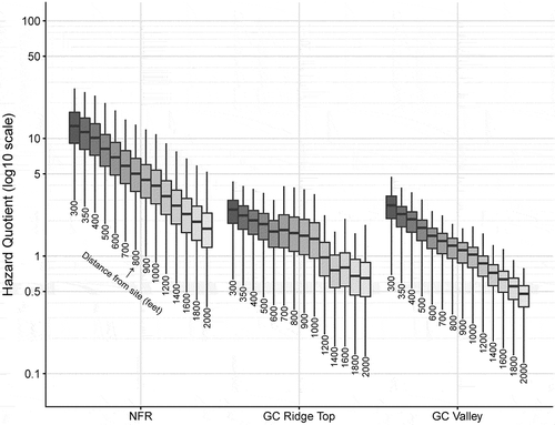
In Figure 5, the generally small differences in HQ distributions between the GC sites result from differences in meteorology (we used the same emissions data at both sites). The acute benzene HQs during flowback are much higher at the NFR site relative to the GC sites; while there are differences in meteorology between the sites, the higher HQs at the NFR site result primarily from higher emissions (see Figure A-1, Supplementary Section A). Figure 5 also illustrates the dependence of HQs on distance. As anticipated, HQs at distances < 500 ft (inside the Colorado setback requirement) were usually higher than those at 500 ft. At these closer locations, as shown in Supplementary Section H, HQs and HIs reached as high as 27, with maximum HQs > 1 for 4-ethyltoluene, n-decane, n-propylbenzene, and m + p-xylene, and maximum HIs > 1 for respiratory and sensory groups, during fracking or flowback at the GC sites (plus the VOCs and groups already mentioned as having values > 1 at 500 ft). Finally, Figure 5 illustrates how the distributions of acute benzene HQs during flowback vary between the three hypothetical sites: median HQs at 500 ft were similar for the two GC sites (within about 30% of each other), while at the NFR site they were approximately 5 times higher. Additionally, the pattern of decreasing HQs with increasing distance differs between sites, owing primarily to differences in meteorological conditions, with the GC ridge-top site showing the least (relative) decrease in acute HQ 500-to-2,000 ft.

VOC emissions, and thus the acute HQs, were generally much lower during O&G production vs. development. Benzene was the only chemical with a maximum acute HQ > 1 during production (2.9 and 1.6 at 150 and 500 ft, respectively, at the NFR site; corresponding HQs at the GC ridge-top site were 2.6 and 1.4, and 2.7 and 1.1 at the GC valley site). HQs were < 1 beyond 600 ft (183 m) from the pad at the GC sites and beyond about 1,200 ft (366 m) for NFR. Hematological toxicity (driven by benzene) was the only critical-effect group with HIs > 1 at any site and distance associated with production.

Incremental subchronic exposures

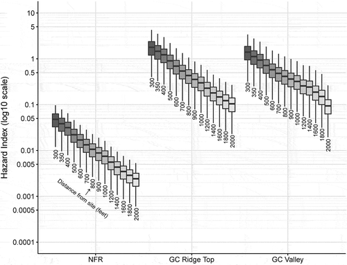
We did not calculate subchronic HQs or HIs for O&G activities lasting > 1 year; potential adverse effects from such long-term exposures are adequately captured by comparison to the generally more health-protective chronic criteria. For O&G development, estimated subchronic exposures to individual VOCs were below subchronic criteria at 500–2,000 ft from all modeling sites. For combined exposures at 500 ft, maximum HIs were > 1 (up to 2.2) for the hematological and neurotoxicity groups at the GC sites during fracking (all pad configurations at the ridge-top site; 1- and 3-acre pads at the valley site), and these HIs > 1 extended to 800 ft (244 m) from the pads and were higher at distances inside the Colorado setback requirement. This can be seen in Figure 6, where distributions of subchronic HIs are plotted for neurotoxicity at the selected receptors during fracking activities at a hypothetical 1-acre pad. The HIs composing the distributions are from across the modeled year (different periods of the year with durations corresponding to assumed activity durations) and the set of individuals. The span of subchronic neurotoxicity HIs during fracking was close to one order of magnitude at all sites and distances. M + p-xylene and n-nonane contributed the most to neurotoxicity effects, while m + p-xylene and benzene contributed the most to hematological effects, with m + p-xylene having an HQ near 1 at both GC sites for the 1-acre scenario. At locations < 500 ft from the pad, maximum HQs or HIs were > 1 for benzene, m + p-xylene, n-nonane, and the respiratory group (in addition to those already mentioned as being > 1 at 500 ft) during fracking and flowback activities individually and during all development activities in sequence (not shown), with maximum HQs near 2 and maximum HIs near 4.3 (we provide in Supplementary Section H the HQs and HIs for individual chemicals and critical-effect groups associated with different pad sizes, at all modeled distances and sites).

Figure 6. Distributions of subchronic non-cancer hazard indices for the neurotoxicity critical-effect group (across the hypothetical population) at distances from the centre of the 1-acre well pad during fracking activities. The bottom and top of the boxes are the 25th and 75th percentiles, respectively; the line inside the box represents the median; and the bottom and top whiskers are the minima and maxima. Notes: log10 = logarithm base 10; NFR = Northern Front Range; GC = Garfield County; GC Ridge Top refers to the BarD site; GC Valley refers to the Rifle site.

Incremental chronic exposures – non-cancer

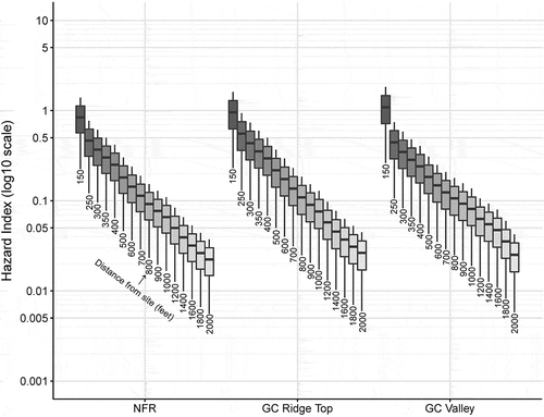
We evaluated chronic non-cancer hazards for two sets of scenarios: those involving O&G production only (the modeled individual is not present for well development), and those involving development and production activities (the individual is present for all activities). During production, emissions are generally much lower than during the highest-emission development activities. Thus, notwithstanding the more demanding chronic health criteria, maximum chronic HQs and HIs were < 1 for production activities at 500 ft from each site, falling to < 0.1 at 2,000 ft. Only at the closest receptor (150 ft, much closer than setback requirements) were the chronic HQs > 1 (1.1–1.2) for benzene during production. At this distance during production, chronic HIs ranged 1.4–1.8 for hematological effects and 1.1–1.3 for neurotoxicity. We provide in Supplementary Section H the HQs and HIs for individual chemicals and critical-effect groups, at all distances.

Figure 7 illustrates the variability in chronic HIs for hematological effects during production at the selected receptors. The distributions are from across the modeled individuals, with modeled exposure durations defined as 1 year (assumed to reflect a 30-year average over the duration of production). The span of HIs was about a factor of 6–8 at all sites and distances. In contrast to the acute and subchronic results, generally the variability in chronic HI was < 15% between sites.

Figure 7. Distributions of chronic non-cancer hazard indices for the hematological critical-effect group (across the hypothetical population) at distances from the centre of the 1-acre well pad during production activities. The bottom and top of the boxes are the 25th and 75th percentiles, respectively; the line inside the box represents the median; and the bottom and top whiskers are the minima and maxima. Notes: log10 = logarithm base 10; NFR = Northern Front Range; GC = Garfield County; GC ridge top refers to the BarD site; GC Valley refers to the Rifle site.

For the combined development-production scenario, long-term exposure varies with pad size; larger pads have longer development periods resulting in higher duration-weighted-average exposures. For 1-acre pads (a single well) and 3-acre pads (8 wells at NFR sites; 16 wells at GC sites), development is completed within weeks to months, so the resulting weighted-average chronic exposures were very similar to those for production alone and were below criteria in all cases.

For 5-acre pads (32 wells), at the GC sites the estimated development time exceeds 1 year, with flowback lasting over a year. During these development scenarios, all chronic HQs were < 1 at ≥ 500 ft, while maximum chronic HIs were > 1 at 500 ft for hematological and neurotoxicity effects (2.1 and 1.5, respectively, at the GC ridge-top site; 1.9 and 1.2 at the GC valley site). Benzene and n-nonane emissions from flowback contributed the bulk of the hematological and neurotoxicity HIs.

Chronic exposures – incremental lifetime cancer risks

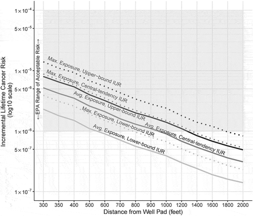
We calculated 70-year incremental lifetime cancer risks associated with exposures to benzene for the 30–32-year combined development-production scenario, utilizing central-tendency and maximum chronic-exposure estimates. Risks were 8–14% higher at the 3-acre pads and 19–40% higher at the 5-acre pads vs. the 1-acre pad, owing to longer durations of development at the larger sites. In areas < 500 ft from the well pad (inside the setback zone), maximum risks (maximum exposures with upper-bound IUR) reached 1.4 × 10⁻⁵ (for 1-acre sites) to 1.6 × 10⁻⁵ (for 5-acre sites), while central-tendency risks (average exposures with central-tendency IUR) were 5.2x10⁻⁶–6.1x10⁻⁶.

All risk estimates fell to ≤ 8.2 × 10⁻⁶ at 500 ft, with central-tendency risks ≤ 3.1 × 10⁻⁶ and falling to ≤ 1.0 × 10⁻⁶ by 1,200 ft. All risks fell to ≤ 1.0 × 10⁻⁶ between 500 ft (average exposures using lower-bound IUR at 1- and 3-acre sites) and 2,000 ft (maximum estimates at all sites).

Figure 8 summarizes the cancer risks calculated at all distances from the GC ridge-top site, assuming a 1-acre pad and utilizing the three IURs (including the lower bound). For this scenario, estimated incremental lifetime cancer risks at 500 ft ranged from 1.1 × 10⁻⁶ (average exposure, lower-bound IUR) to 6.8 × 10⁻⁶ (maximum value). As shown in the full results presented in Supplementary Section I, maximum estimated lifetime cancer risks at 500 ft were 5.7 × 10⁻⁶ and 5.6 × 10⁻⁶ at the GC valley and NFR sites, respectively, decreasing with distance in a manner similar to that for the GC ridge-top site. Also, estimated cancer risks increased slightly with size of development pad, owing to longer durations of development activities.

Figure 8. Incremental lifetime cancer risks from benzene exposure for average- and maximum-exposed hypothetical individuals at distances from the centre of the well pad during all activities in sequence at the Garfield County ridge-top site (1-acre development pad, 1-acre production pad). X-axis is not to scale. Grey box indicates the U.S. Environmental Protection Agency’s range of acceptable cancer risk. Notes: Avg. = average; max. = maximum; IUR = inhalation unit risk.

Uncertainties and limitations

In this section, we summarize the major uncertainties and limitations of our assessment. See Supplementary Section F for additional analyses of the uncertainties and sensitivities of the assessment to various methodological choices and input parameters, and Supplementary Section G for a discussion of sensitivity analyses conducted on modeling inputs.

We estimate the emission rates, which directly and proportionally affect risk estimates, represented the highest uncertainty in the assessment, having perhaps ≥ 0.5 orders of magnitude of potential influence on the results. Emission measurements were at a limited number of sites, so we cannot be certain that they are representative of the full, real-world distribution of O&G emission and dispersion scenarios, particularly at the upper tail (as with any assessment, there is considerable uncertainty at the extreme tails of the data and outputs). O&G emissions can be highly variable with respect to configuration and operational practices, and the measurements reflected this high variability (as seen previously in Adgate, Goldstein, and McKenzie 2014; Allen 2016; Brantley, Thoma, and Eisele 2015; McMullin et al. 2018; Thompson et al. 2017). When we estimated 1-hour-avearge emission rates, there was uncertainty in assuming the means were similar to those of the 3-minute measurements and fitting the values to a lognormal distribution.

The limited sampling and high variability in measured emissions necessitated use of stochastic methods to capture the resulting variabilities in exposure and generalize the results to different O&G-activity durations and geographic and meteorological settings. While these meteorology settings included several years of hourly meteorology in different locations, including wind speeds as low as 0.2 meters per second, we may not have captured all possible weather conditions (an estimated 2–3-fold uncertainty).

These uncertainties and limitations particularly affect the interpretation of “maximum” HQs and HIs. Maximum exposures, as defined in this assessment, occur only at the most-exposed locations during atypical times when simulations created a confluence of very conservative meteorological conditions, unusually high emissions, and personal activities leading to exposures far above average. Maximum exposures also assume individuals reside at the most-exposed locations. While these conditions are possible according to our assumptions and input data (and indeed they are the health-protective focus of our assessment), as outputs in the upper tails of our modeling results, they are not representative of “typical” exposures. Distributions of typical exposures will generally be shifted toward lower values, sometimes much lower, at other receptors. Additional analyses with site-specific monitoring and meteorological data would better characterize the relationship between the highest and typical exposures during well development and production (analyses such as McKenzie et al. 2012; Colborn et al. 2014 but including information on acute timescales and, in the case of Colborn et al. 2014, with measurements within a half-mile of the well-pad centre).

Previous studies and reviews suggested O&G emissions can contribute to exceedances of regulatory or guidance levels of health and ecological welfare on a local and regional scale (e.g., Shonkoff, Hays, and Finkel 2014; Thompson et al. 2017). While our study has the advantage of helping to understand the contribution of a single O&G facility toward an individual’s exposure, multiple O&G facilities are increasingly intermingled with residential and recreational areas. The large numbers of chemical exposures experienced by any individual, across short and especially long (chronic) time scales, and their variable and sometimes compounding effects on human health, are complex and uncertain.

Another limitation of our analysis is that we used a limited number of generic well-pad configurations to represent several variations in possible release conditions, but risk estimates (particularly those close to the well pad) can be sensitive to the exact locations and specifications of the emission sources (e.g., we estimated a < 3-fold potential risk-assessment uncertainty related to the AERMOD dispersion modeling, including source characterization). We did not utilize decline curves to account for variations in emissions during O&G production (as they are uncertain and dependent on the site and operator), nor did we utilize algorithms for downwash due to any obstructions that might be present (e.g., sound walls at development sites). Additional monitoring campaigns and modeling efforts near a variety of well-pad configurations and structures would provide important additional data on potential health risks.

Considering these limitations, the exposure concentrations we generated, while representative of higher-end values that would be seen at the modeling sites as-configured, do not constitute real-time measurements. We believe the exposure distributions are realistic, providing reliable summary statistics for the time frames examined, but new studies collecting additional exposure data would add to the body of knowledge. There is also some degree of uncertainty (probably < 2 fold) associated with applying APEX to estimate personal exposures, but on aggregate, these APEX-related uncertainties are small compared to those associated with emission estimation, air modeling, and health-criteria values.

There is an unavoidable degree of uncertainty associated with the values of health criteria and cancer slope factors used to estimate HQs, HIs, and lifetime cancer risks. The level of uncertainty associated with such values is generally estimated to be about one order of magnitude, and the toxic effects of some chemicals are currently less well understood than others like benzene. The HI estimates did not include examination of synergistic effects.

A final limitation of this study is it does not include all airborne chemicals previously detected near O&G sites. The canister sampling methodology used to characterize emissions measured only hydrocarbons; levels of polar oxygen-, sulfur-, and nitrogen-containing compounds were not quantified, though some (formaldehyde and acetaldehyde) have been frequently observed near O&G sites, and they are known or suspected human carcinogens (McMullin et al. 2018). We also did not calculate cancer risks for several chemicals in our assessment (styrene, isoprene, and ethylbenzene) classified by IARC or EPA as “possible” or “probable” human carcinogens, but for which human exposure-response models were not available. Exclusion of chemicals from our analysis results in lower estimates of HIs and total cancer risks than if we had included them.

Conclusions

Our study coupled stochastic dispersion modeling of emission rates with probabilistic risk-assessment methods to illustrate the potential non-cancer hazards and cancer risks associated with air emissions of certain VOCs from individual sites of O&G development and production in Colorado under plausible highest-exposure scenarios. The results will help in evaluating the efficacy of setback distances in protecting public health from such emissions. The emission studies (CSU 2016a, 2016b; Hecobian et al. 2019) utilized here were among the first of their kind in the US to use the TRM near individual facilities to characterize per-facility emission rates from individual phases of O&G development and production. Their measurements are likely comparable to similar sites elsewhere. The measurements were source-attributable because the facility’s emission plume was identified with a mobile tracker, and other nearby chemical signals were removed via an upwind background monitor. This is in contrast to typical monitoring data (e.g., those used by Colborn et al. 2014; Gilman et al. 2013; Halliday et al. 2016; Long, Briggs, and Bamgbose 2019; McKenzie et al. 2018, 2012; McMullin et al. 2018; Swarthout et al. 2013; Thompson, Hueber, and Helmig 2014) which measure the ambient air both within and outside the plume (depending on conditions) and cannot necessarily differentiate a target source of emissions from other nearby emissions. Our stochastic approach to dispersion modeling, whereby we combined the on-site-measured emissions data with multiple datasets of variable meteorology, has the advantage of generating thousands of credible and representative short- and long-term VOC air-concentration scenarios at hundreds of possible exposure locations – many more than can be reasonably observed with monitoring. These include myriad acute (1-hour) scenarios that have been understudied to-date in O&G risk assessments. Further, rather than assuming constant exposure to outdoor air (as was done, for example, by McKenzie et al. 2012; McMullin et al. 2018), we estimated individual exposures across MEs using the state-of-the-science APEX model with time-activity-pattern data (including surveys from Coloradans) and distributions of ME PENs based on chemical volatility. From these data, we derived detailed distributions of acute, subchronic, and chronic exposures for each modeled site, pad size, and exposure distance. We compared these exposures to toxicity criteria issued by federal and state agencies, chosen so as to generally prefer federal criteria based on the most current and complete data available and state-of-the-science methods.

Acute exposures were of greatest concern, primarily during O&G development and for a limited set of VOCs and critical-effect groups, sometimes at distances out to 2,000 ft from the well pad. While most acute HQs and HIs were < 1 for most VOCs and critical-effect groups, our results suggest the potential for HQs and HIs > 1, sometimes > 10, for several VOCs (particularly benzene and 2-ethyltoluene) and critical-effect groups (particularly neurological and hematological effects), during O&G development (particularly drilling and flowback). Benzene HQs, and hematological HIs driven by benzene emissions, were slightly > 1 during O&G production. These findings support increased concern for adverse effects in the exposed individuals, although the exact probability or severity of adverse effects cannot be estimated. Our results contrast somewhat with those of McMullin et al. (2018), who utilized ambient monitoring data and found all acute exposures to outdoor air were below criteria, except for the conservative “all-VOC” HI estimate (which we did not calculate) which was 1.2. However, nearly all monitoring data utilized by McMullin et al. (2018) were > 500 ft from the closest wells, and observations ≤ 500 ft were limited to regions of O&G activity rather than site-specific studies and were targeting either the lower-emitting production activities or were 24-hour integrated measurements rather than 1-hour averages. However, as in our study, McMullin et al. (2018) found benzene to be among the chemicals of highest relative concern and most VOCs corresponded to acute exposures far below criteria levels.

Nearly all HQs and HIs for subchronic effects were < 1 at ≥ 500 ft from the well pads. During fracking, subchronic HIs for hematological and neurotoxicity effects slightly exceeded 1 at 800 ft from the two GC locations. These findings were generally similar to those of McKenzie et al. (2012), who utilized ambient monitoring data close to well sources and found higher-end subchronic exposures to outdoor air (for people living within 0.5 miles of wells) that slightly exceeded criteria values for 1,3,5-trimethylbenzene (which had among the highest subchronic HQs in our study as well, though below criteria) and that lead to HIs ≤ 4 for several critical effects (particularly neurotoxicity and hematological).

Emissions during well production did not lead to chronic exposures above criteria levels at ≥ 250 ft from well pads. Chronic exposures due to well development lasting > 1 year resulted in chronic HIs for hematological and neurological effects that slightly exceeded 1 at 500 ft from 5-acre pads. These findings generally match those of McMullin et al. (2018) and McKenzie et al. (2012), who found for constant exposure to outdoor air that all chronic HQs, and all HIs for individual critical-effect groups, were below criteria levels.

Our largest estimated incremental cancer risks associated with benzene exposure were < 2.0 × 10⁻⁵ at all distances. We estimated central-tendency risks (average exposure, central-tendency IUR) to be 2.1x10⁻⁶–3.1x10⁻⁶ (depending on pad size) at the 500-ft location most often downwind from the pad, decreasing to < 1.0 × 10⁻⁶ by 1,000–1,200 ft. The largest risk estimates fell below 1.0 × 10⁻⁶ by 2,000 ft. McKenzie et al. (2012) estimated similar benzene cancer risks (3.3x10⁻⁶–8.7x10⁻⁶, depending on the concentration used for constant exposure to outdoor air); risk estimates due to other chemicals were smaller than for benzene. McMullin et al. (2018) estimated benzene cancer risks in a higher range (1.0x10⁻⁵–3.6x10⁻⁵) due to constant exposure to outdoor air, which are similar to levels we estimated inside the 500-ft setback (up to 1.6 × 10⁻⁵); here, too, risk estimates were highest for benzene.

These findings provide important information related to potential health hazards associated with O&G development and production activities in Colorado, and they shed light on the specific activities and chemicals of most concern for further analyses of such risks. These include, in particular, benzene and 2-ethyltoluene emissions during drilling and flowback, and hematological effects during most development phases. To a lesser degree, these also include 3-ethyltoluene and toluene emissions and neurotoxicity and respiratory effects during drilling and flowback; hematological and neurotoxicity effects during fracking (driven primarily by benzene, m + p-xylene, and n-nonane emissions); and hematological and neurotoxicity effects during extended development phases at large multi-well sites (driven primarily by benzene and n-nonane emissions). Acute exposures were of greatest concern: acute HQs and HIs were generally much higher than subchronic and chronic HQs and HIs, with acute values > 1 in some cases as far out as 2,000 ft from the well pad (our maximum modeled distance).

Relative to monitoring studies, we have high confidence that these chemical signals are attributed directly to O&G activities on the target well pad, due to the TRM used to derive on-site O&G emissions during specific O&G activities. We also have high confidence that the estimated exposures reasonably represent some real-life exposures that could be experienced by people living near O&G facilities, due to the stochastic approaches to dispersion and ME assessment allowing the generation of thousands of acute-to-chronic exposure scenarios for individuals across the 2,000-ft radius. These approaches and findings can be used to further evaluate data needs and to support refinement of setback distances.

Acknowledgments

The authors appreciate the substantial support of CDPHE as well as Arsineh Hecobian and Jeff Collett at CSU. We also appreciate the support of George Agyeman-Badu, Louise Assem, Dave Burch, Anna Engstrom, Jeremy Frye, Sophie Hearn, Kevin Hobbie, Heidi Hubbard, Kristen McKinley, Whitney Mitchell, Revathi Muralidharan, Delaney Reilly, Alessandria Schumacher, Courtney Skuce, Anna Stamatogiannakis, and Nicole Vetter. CDPHE provided some of the data used in the assessment as well as some input into study design.

Supplementary data

Supplemental data for this article can be accessed on the publisher's website..

Additional information

Funding

This work was supported by the Colorado Department of Public Health and Environment [CMS Routing Number 17 FHHA 97218; PO,FAAA,201800010964].

Notes on contributors

Chris Holder

Chris Holder is an exposure scientist at ICF in Durham, NC, USA.

John Hader

John Hader was an exposure scientist at ICF in Durham, NC, USA, and is now a Ph.D. candidate at the Stockholm University in Stockholm, Sweden.

Raga Avanasi

Raga Avanasi was an exposure scientist at ICF in Durham, NC, USA.

Tao Hong

Tao Hong was a programmer at ICF in San Francisco, CA, USA, and he is now an independent researcher in Belmont, CA, USA.

Ed Carr

Ed Carr is an air quality scientist at ICF in San Francisco, CA, USA.

Bill Mendez

Bill Mendez is a toxicologist at ICF in Fairfax, VA, USA.

Jessica Wignall

Jessica Wignall is a toxicologist at ICF in Burlington, VT, USA.

Graham Glen

Graham Glen is an exposure scientist at ICF in Durham, NC, USA.

Belle Guelden

Belle Guelden is an air quality scientist at ICF in Tiburon, CA, USA.

Yihua Wei

Yihua Wei is an air quality scientist at ICF in San Francisco, CA, USA.

References

- Adgate, J. L., B. D. Goldstein, and L. M. McKenzie. 2014. Potential public health hazards, exposures and health effects from unconventional natural gas development. Enviorn. Sci. Technol. 48 (15):8307–20. doi:10.1021/es404621d.
- Allen, D. T. 2016. Emissions from oil and gas operations in the United States and their air quality implications. J. Air Waste Manage. Assoc. 66 (6):549–75. doi:10.1080/10962247.2016.1171263.
- ATSDR (Agency for Toxic Substances and Disease Registry). 2018. Framework for assessing health impacts of multiple chemicals and other stressors (update). February. https://www.atsdr.cdc.gov/interactionprofiles/ip-ga/ipga.pdf.
- Balter, B. M., and M. V. Faminskaya. 2016. Irregularly emitting air pollution sources: Acute health risk assessment using AERMOD and the Monte Carlo approach to emission rate. Air Quality Atmos. Health 10:401–09. doi:10.1007/s11869-016-0428-x.
- Bowman, C., and R. Dhammapala. 2011. A Monte Carlo approach to estimating impacts from highly intermittent sources on short term standards. Presented at the Northwest International Air Quality Environmental Science and Technology Consortium, Pullman, Washington, June 1.
- Brantley, H. L., E. D. Thoma, and A. P. Eisele. 2015. Assessment of volatile organic compound and hazardous air pollutant emissions from oil and natural gas well pads using mobile remote and on-site direct measurements. J. Air Waste Manage. Assoc. 65 (9):1072–82. doi:10.1080/10962247.2015.1056888.
- Casey, J. A., D. A. Savitz, S. G. Rasmussen, E. L. Ogburn, J. Pollak, D. G. Mercer, and B. S. Schwartz. 2016. Unconventional natural gas development and birth outcomes in Pennsylvania, USA. Epidemiology 27 (2):163–72. doi:10.1097/EDE.0000000000000387.
- CODOLA (Colorado Department of Local Affairs). 2019. County and municipal population time series. accessed May 14, 2019. https://demography.dola.colorado.gov/population/data/county-muni-timeseries/.
- COGCC (Colorado Oil and Gas Conservation Commission). 2007. Greater Wattenberg area baseline study, greater Wattenberg area, Colorado. http://cogcc.state.co.us/documents/library/AreaReports/DenverBasin/GWA/Greater_Wattenberg_Baseline_Study_Report_062007.pdf.
- COGCC. 2019. Colorado Oil and Gas Information System (COGIS). accessed May 14, 2019. http://cogcc.state.co.us/data.html#/cogis.
- Colborn, T., K. Schultz, L. Herrick, and C. Kwiatkowski. 2014. An exploratory study of air quality near natural gas operations. Human Ecol. Risk Assess. 20 (1):86–105. doi:10.1080/10807039.2012.749447.
- CSU (Colorado State University). 2016a. Characterizing emissions from natural gas drilling and well completion operations in Garfield County, CO. https://www.garfield-county.com/air-quality/documents/CSU-GarCo-Report-Final.pdf.
- CSU. 2016b. North front range oil and gas air pollutant emission and dispersion study. https://www.colorado.gov/airquality/tech_doc_repository.aspx?action=open&file=CSU_NFR_Report_Final_20160908.pdf.
- Czolowski, E. D., R. L. Santoro, T. Srebotnjak, and S. B. C. Shonkoff. 2017. Toward consistent methodology to quantify populations in proximity to oil and gas development: A national spatial analysis and review. Environ. Health Perspect. 125:086004. doi:10.1289/EHP1535.
- EPA. 2000. IRIS chemical assessment summary, benzene. EPA National Center for Environmental Assessment. https://cfpub.epa.gov/ncea/iris/iris_documents/documents/subst/0276_summary.pdf#nameddest=woe.
- EPA. 2009. Risk assessment guidance for superfund. Volume I: Human health evaluation Manual (Part F, supplemental guidance for inhalation risk assessment). Final. January. EPA-450-R-070-002, OSWER 9285. EPA Office of Superfund Remediation and Technology Innovation. 7–82. https://www.epa.gov/sites/production/files/2015-09/documents/partf_200901_final.pdf.
- EPA. 2016. The Consolidated Human Activity Database (CHAD), documentation and users’ guide. EPA Office of Air Quality Planning and Standards and National Exposure Research Laboratory.
- EPA. 2017. Air Pollutants Exposure Model Documentation (APEX, version 5), Volume I: User’s guide, Volume II: Technical support document. EPA-452/R-17-001a,b. EPA Office of Air Quality Planning and Standards. https://www.epa.gov/fera/apex-user-guides.
- EPA. 2018a. Air quality dispersion modeling - Preferred and recommended nodels. accessed December 12, 2018. https://www.epa.gov/scram/air-quality-dispersion-modeling-preferred-and-recommended-models#aermod.
- EPA. 2018b. Risk and exposure assessment for the review of the primary national ambient air quality standard for sulfur oxides. EPA-452/R-18-003. EPA Office of Air Quality Planning and Standards. https://www.epa.gov/sites/production/files/2018-05/documents/primary_so2_naaqs_-_final_rea_-_may_2018.pdf.
- EPA (U.S. Environmental Protection Agency). 1994. Use of Monte Carlo simulation in risk assessments. EPA Region 3. EPA903-F-94-001. https://www.epa.gov/risk/use-monte-carlo-simulation-risk-assessments.
- Gilman, J. B., B. M. Lerner, W. C. Kuster, and J. A. de Gouw. 2013. Source signature of volatile organic compounds from oil and natural gas operations in northeastern Colorado. Environ. Sci. Technol. 47 (3):1297–305. doi:10.1021/es304119a.
- Guerra, S. A. 2014. Innovative dispersion modeling practices to achieve a reasonable level of conservatism in AERMOD modeling demonstrations. EM Magazine. 12:24–29. http://pubs.awma.org/flip/EM-Dec-2014/guerra.pdf.
- Haley, M., M. McCawley, A. C. Epstein, B. Arrington, and E. F. Bjerke. 2016. Adequacy of current state setbacks for directional high-volume hydraulic fracturing in the Marcellus, Barnett, and Niobrara shale plays. Environ. Health Perspect. 124:1323–33. doi:10.1289/ehp.1510547.
- Halliday, H. S., A. M. Thompson, A. Wisthaler, D. Blake, R. S. Hornbrook, T. Mikoviny, M. Müller, P. Eichler, E. C. Apel, and A. J. Hills. 2016. Atmospheric benzene observations from oil and gas production in the Denver Julesburg Basin in July and August 2014. J. Geophysical. Res. 121:11055–74. doi:10.1002/2016JD025327.
- Hecobian, A., A. L. Clements, K.B. Shonkwiler, Y. Zhou, L. P. MacDonald, N. Hilliard, B. L. Wells, B. Bibeau, J. M. Ham, J. R. Pierce, and J. L. Collett Jr. 2019. Air toxics and other volatile organic compound emissions from unconventional oil and gas development. Environ. Sci. Technol Letters.
- Hill, E. L. 2018. Shale gas development and infant health: Evidence from Pennsylvania. J. Health Econ. 61:134–50. doi:10.1016/j.healeco.2018.07.004.
- Lamb, B. K., J. B. McManus, J. H. Shorter, C. E. Kolb, B. Mosher, R. C. Harriss, E. Allwine, D. Blaha, T. Howard, A. Guenter, et al. 1995. Development of atmospheric tracer methods to measure methane emissions from natural gas facilities and urban areas. Environ. Sci. Technol. 29:1468–79. doi:10.1021/es00006a007.
- Li, H. L., G. H. Huang, and Y. Zou. 2008. An integrated fuzzy-stochastic modeling approach for assessing health-impact risk from air pollution. Stochastic Environ. Res. Risk Assess. 22:789–803. doi:10.1007/s00477-007-0187-1.
- Lonati, G., and F. Zanoni. 2013. Monte-Carlo human health risk assessment of mercury emissions from a MSW gasification plant. Waste Manag. 33:347–55. doi:10.1016/j.wasman.2012.10.015.
- Long, C. M., N. L. Briggs, and I. A. Bamgbose. 2019. Synthesis and health-based evaluation of ambient air monitoring data for the Marcellus Shale region. J. Air Waste Manage. Assoc. 69:527–47. doi:10.1080/10962247.2019.1572551.
- Maryland School of Public Health. 2014. Potential public health impacts of natural gas development and production in the Marcellus Shale in western Maryland. http://www.marcellushealth.org/uploads/2/4/0/8/24086586/final_report_08.15.2014.pdf.
- McKenzie, L. M., B. D. Blair, J. Hughes, W. B. Allshouse, N. Blake, D. Helmig, P. Milmoe, H. Halliday, D. R. Blake, and J. L. Adgate. 2018. Ambient nonmethane hydrocarbon levels along Colorado’s northern front range: Acute and chronic health risks. Environ. Sci. Technol. 52 (8):4514–25. doi:10.1021/acs.est.7b05983.
- McKenzie, L. M., R. Guo, R. Z. Witter, D. A. Satvitz, L. S. Newman, and J. L. Adgate. 2014. Birth outcomes and maternal residential proximity to natural gas development in rural Colorado. Environ. Health Perspect. 122:412–17. doi:10.1289/ehp.1306722.
- McKenzie, L. M., R. Z. Witter, L. S. Newman, and J. L. Adgate. 2012. Human health risk assessment of air emissions from development of unconventional natural gas resources. Sci. Total Enviorn. 424:79–87. doi:10.1016/j.scitotenv.2012.02.018.
- McKenzie, L. M., W. B. Allshouse, T. Burke, B. D. Blair, and J. L. Adgate. 2016. Population size, growth, and environmental justice near oil and gas wells in Colorado. Environ. Sci. Technol. 50:11471–80. doi:10.1021/acs.est.6b04391.
- McKenzie, L. M., W. B. Allshouse, T. E. Byers, E. J. Bedrick, B. Serdar, and J. L. Adgate. 2017. Childhood hematologic cancer and residential proximity to oil and gas development. PLoS ONE 12 (2):e0170423. doi:10.1371/journal.pone.0170423.
- McMullin, T., A. Bamber, B. Bon, D. Vigil, and M. Van Dyke. 2018. Exposures and health risks from volatile organic compounds in communities located near oil and gas exploration and production activities in Colorado (USA). Int. J. Environ. Res. Public Health 15:1500. doi:10.3390/ijerph15071500.
- OEHHA (California Office of Environmental Health Hazard Assessment). 2009. Technical support document for cancer potency factors. May. https://oehha.ca.gov/air/crnr/technical-support-document-cancer-potency-factors-2009.
- Paine, R., C. Szembek, D. Heinold, E. Knipping, and N. Kumar. 2014. Emissions Variability Processor (EMVAP): Design, evaluation, and application. J. Air Waste Manage. Assoc. 64:1390–402. doi:10.1080/10962247.2014.956159.
- Rabinowitz, P. M., I. B. Slizovskiy, V. Lamers, S. J. Trufan, T. R. Holford, J. D. Dziura, P. N. Peduzzi, M. J. Kane, J. S. Reif, T. R. Weiss, et al. 2015. Proximity to natural gas wells and reported health status: Results of a household survey in Washington County, Pennsylvania. Environ. Health Perspect. 123:21–26. doi:10.1289/ehp.1307732.
- Shonkoff, S. B. C., J. Hays, and M. L. Finkel. 2014. Environmental public health dimensions of shale and tight gas development. Environ. Health Perspect. 122:787–95. doi:10.1289/ehp.1307866.
- Small, M. J., P. C. Stern, E. Bomberg, S. M. Christopherson, B. D. Goldstein, A. L. Israel, R. B. Jackson, A. Krupnick, M. S. Mauter, J. Nash, et al. 2014. Risks and risk governance in unconventional shale gas development. Environ. Sci. Technol. 48 (15):8289–97. doi:10.1021/es502111u.
- Stacy, S. L., L. L. Brink, J. C. Larkin, Y. Sadovsky, B. D. Goldstein, B. R. Pitt, and E. O. Talbott. 2015. Perinatal outcomes and unconventional natural gas operations in southwest Pennsylvania. PLoS ONE 10 (6):e0126425. doi:10.1371/journal.pone.0126425.
- Swarthout, R. F., R. S. Russo, Y. Zhou, A. H. Hart, and B. C. Sive. 2013. Volatile organic compound distributions during the NACHTT campaign at the boulder atmospheric observatory: Influence of urban and natural gas sources. J. Geophysical. Res. 118 (18):10,614–10,637. doi:10.1002/jgrd.50722.
- Thompson, C. R., J. Hueber, and D. Helmig. 2014. Influence of oil and gas emissions on ambient atmospheric non-methane hydrocarbons in residential areas of northeastern Colorado. Elem. Sci. Anthropocene 2:000035. doi:10.12952/journal.elementa.000.
- Thompson, T. M., D. Shepherd, A. Stacy, M. G. Barna, and B. A. Schichtel. 2017. Modeling to evaluate contribution of oil and gas emissions to air pollution. J. Air Waste Manage. Assoc. 67 (4):445–61. doi:10.1080/10962247.2016.1251508.
- Tustin, A. W., A. G. Hirsch, S. G. Rasmussen, J. A. Casey, K. Bandeen-Roche, and B. S. Schwartz. 2017. Associations between unconventional natural gas development and nasal and sinus, migraine headache, and fatigue symptoms in Pennsylvania. Environ. Health Perspect. 125:189–97. doi:10.1289/EHP281.
- Wells, B. 2015. The validation of emission rate estimation methods. Master's Thesis, Colorado State University, Department of Atmospheric Sciences, Fort Collins, Colorado.
- Whitworth, K. W., A. K. Marshall, and E. Symanski. 2017. Maternal residential proximity to unconventional gas development and perinatal outcomes among a diverse urban population in Texas. PLoS ONE 12 (7):e0180966. doi:10.1371/journal.pone.0180966.
- Whitworth, K. W., A. K. Marshall, and E. Symanski. 2018. Drilling and production activity related to unconventional gas development and severity of preterm birth. Environ. Health Perspect. 126:037001–08. doi:10.1289/EHP2622.