Meteorological modeling relevant to mesoscale and regional air quality applications: a review

ABSTRACT

The highest correlative relations for air pollution levels are often with meteorological variables such as temperature and wind speed. Today, sophisticated gridded high-resolution meteorological models are used to produce meteorological fields that drive chemical transport models for air quality management. Errors in specification of the physical atmosphere such as temperature, clouds and winds can affect the air quality predictions. Additionally, the efficiency and efficacy of emission control strategies can be compromised by errors in the meteorological fields. In this paper, the role of meteorology in air quality behavior, primarily from the viewpoint of regional ozone modeling as carried out in the U.S., is reviewed. Particular attention is given to physics and new techniques for improving meteorological model performance. Uncertainties in model turbulent mixing in the nighttime boundary layer, where large model differences exist, are examined. The role of spatial mesoscale features such as topography and land/water systems in models are discussed. The nocturnal low-level jet, a mesoscale temporal and spatial feature, and its impact on air quality are examined. Traditional air quality concerns have focused on synoptic conditions at the center of high-pressure systems. However, high ozone levels have also been associated with stationary fronts. The ability of models to capture mesoscale structure and yet retain synoptic structure and its timing is challenging. Data assimilation and its ability to improve model performance are examined. Particular attention is given to vertical nudging strategies that can affect formation of the nocturnal low-level jets. Finally, clouds can have a major impact on air quality since insolation impacts temperature, biogenic emissions and photolysis rates and extremes in stability. Traditional techniques, which attempt to insert cloud water where there is not dynamical support, can lead to additional errors. New dynamical approaches for improving model cloud performance are discussed.

Implications: This article shows that there has been a considerable improvement in meteorological models used for air quality simulations. In particular, improvement in the tools for incorporating both traditional observations and new satellite data for retrospective studies has been beneficial to air quality community. However, while this trend is continuing, many challenges remain. As an example, due to having many options available in configuring a model simulation, there is a need to evaluate and recommend sets of options that provide important performance measures.

Introduction

Since the passage of the Clean Air Act of 1970 air quality models have played a major role in air quality assessment and regulation. Early models for control strategy testing (e.g. State Implementation Plans – SIPs) were relatively simple, such as roll-back models for particulates (Larsen 1961) or EKMA curves for ozone. In addition, the emphasis often was on industrial and power plant stack short-term modeling for SO_2. Today, primarily for ozone and fine particles, sophisticated gridded high-resolution (less than 36 km) models are used for control strategy development and for air quality impact assessments. These models include a physical atmosphere (meteorology) model coupled with an atmospheric chemistry (air quality) model. In the present paper, we use the term physical atmosphere as being the atmospheric components that are included in the meteorological model and chemical species that impact photochemical radiation. It is the purpose of this review paper to examine the role of the regional physical atmosphere on air quality and the development of modeling techniques to improve the representation of the regional physical atmosphere in air quality studies.

Examining the physical atmosphere and its impact on air quality is a very broad undertaking that ranges from peak concentrations from individual plumes, to radionuclide exposure, to acid deposition and global chemistry predictions. While the issues discussed below may have relevance to these problems and international air pollution issues, here we examine the regional physical atmosphere largely in the context of ozone control strategy in the U.S. This has been a major focus in the last 20 years by EPA, state and local air pollution regulatory agencies in the U.S. It is also noted that today’s models, with small grid sizes and improved physics, can represent parts of the mesoscale energy spectrum much more completely than 25 years ago.

Some of the previous reviews of meteorology and air quality, including Pielke and Uliasz (1998), Seaman (2000), and Hanna and Yang (2001), provide additional information beyond that provided in this review. Seaman (2000) covered many of the topics discussed here and provided additional perspective, discussion and references with particular emphasis on data assimilation. There have also been reviews that emphasize air quality modeling with emphasis on chemical/meteorological mechanisms and model inputs (Russell and Dennis 2000). Reviews of specific meteorological settings have also been performed. Vardoulakis et al. (2003) reviewed street canyon modeling. Parrish et al. (2011) and Ching (2013) review heat island and mega-city effects. Weil, Sykes, and Venkatram (1992) and Hanna (1994) examined the specifics of evaluation methods for meteorological and air quality models. There have been several reviews of the meteorology and techniques for point source plume modeling, including Eliassen (1980), Wilson and Sawford (1996), and Holmes and Morawska (2006). As wildfires have become important for health concerns and ozone production, modeling of wildfires and their relation to meteorology has also been an important review topic (Goodrick et al. 2013).

Impact of the physical atmosphere on air quality

Statistical analyses (Camalier, Cox, and Dolwick 2007; Cox and Chu 1996) generally show that physical parameters, especially temperature and wind speed, have high correlative relationships with ozone concentrations. Here, the physical and chemical reasons for these high correlations, with an emphasis on ozone, are reviewed in order to clarify the important physical characteristics that need fidelity in current sophisticated modeling systems.

Wind speed

Wind speed is the fundamental variable in controlling most scenarios involving regional primary and secondary air pollutant concentrations. Winds influence both air pollutant and precursor concentrations. As noted by Niemeyer (1960), for continuous releases – “The volume of air into which contaminants are emitted is directly proportional to wind velocity, and the concentration of contaminants is generally inversely proportional to wind speed. If the wind speed doubles, other conditions being equal, the pollutants are emitted into twice the volume of air downstream from the source“. For continuous releases, this concept leads to an inverse relation (1/u) of concentration to wind speed (u). This mathematical relationship is used in box models or steady state Gaussian models, but not for instantaneous releases. For modern time-dependent grid models, the wind speed relation enters through the differential advection terms, and time-averaged concentrations are related to the time an air parcel stays over the source region.

Temperature

Probably the most important, but complex, meteorological parameter for ozone prediction is temperature (Camalier, Cox, and Dolwick 2007). Mostly, all statistical correlative models for ozone show steep linear relations between maximum temperature and ozone levels (Cox and Chu 1996; Dueñas et al. 2002; Vukovich 1994) except at extremely high temperatures (above the 95 percentile). For example, Vukovich (1994) and O’Connor, Roelle, and Aneja (2005), in separate studies in the Eastern U.S., showed that during July and August (what the authors considered the ozone season), of all meteorological variables, maximum temperature had the highest correlation with ozone, with correlations being 0.91 and 0.94, respectively. Rasmussen et al. (2012) reviewed the origins of these temperature relationships. There are confounding issues that make temperature such a highly correlative variable. Part of the temperature–ozone relationship may be tied to wind speed. When wind speeds are low, such as under high-pressure systems, this can lead to high maximum temperatures and low ventilation. Temperature also affects precursors to ozone production, including NO and volatile organic compounds (VOCs) levels. Temperature impacts chemical chain links through thermal decomposition of nitrates (e.g. Sillman and Samson 1995) allowing reuse of NO in ozone production. High temperatures are also associated with clear skies, which can thus enhance photochemical production (Pour‐Biazar et al. 2007). Indirectly, temperature can impact biogenic VOC emissions (Guenther et al. 1993; Lamb et al. 1987) as well as anthropogenic VOC evaporation (Rubin et al. 2006). NO_x emissions can also be increased at higher temperature due to utility cooling demand. There is some evidence of ozone suppression at extreme high temperatures (Shen, Mickley, and Gilleland 2016). This may be due to a fall-off in biogenic emissions due to stress or depletion of nitrate species affecting slopes of ozone reservoirs (Steiner et al. 2010). Shen, Mickley, and Gilleland (2016), however, discounted these chemical processes in favor of meteorological reasons, though the specific meteorological path was not defined. They generally hypothesized that the linearity between ozone and temperature, perhaps through relations to other meteorological variables (solar radiation, stagnation, etc.), breaks down. One mitigating meteorological factor may be increased mixing heights or free convective cloud venting at high temperatures (Holzworth 1972).

Planetary boundary layer (PBL) height

The role of mixed layer height is also fundamental to air pollution concentrations, in that it controls the volume into which emissions or precursors are mixed (Holzworth 1967). Mixing height (H) has been used with wind speed to provide a measure of air pollution potential through the ventilation parameter – V = HxU, where U is the mixed layer average wind speed. Larger values of ventilation infer lower concentrations for continuous releases. When the boundary layer heights reach the lifting condensation level, or level of free convection, cloud processes can control mixed layer heights (Ching and Alkezweeny 1986; Seaman 2000).

Humidity

Water vapor can also have an impact on air quality, both directly and indirectly. In general, higher humidity tends to be inversely related to ozone but the relationship and certainty is not as high as with temperature. Humidity can decrease ozone through terminating chemical chain lengths (Dueñas et al. 2002) and through nitrate aerosol formation. Indirectly, higher relative humidity can be associated with increased cloud cover reducing photochemistry. Higher humidity can also be related to higher soil moisture values, which lower surface temperature. Higher humidity and higher soil moisture can also enhance surface deposition of ozone on vegetative surfaces through greater stomatal uptake.

Cloud cover

Cloud cover can also be an important variable in some scenarios, especially for ozone. Vukovich (1994) showed that sky cover had the highest negative correlation with summer ozone in the Eastern U.S. Cloud cover directly affects both daytime and nighttime temperature. Increased cloud cover decreases daytime insolation and suppresses maximum temperature. It reduces daytime boundary layer turbulence by suppressing thermal convection. However, cloud cover increases nighttime temperature (Dai, Trenberth, and Karl 1999) through downward infrared radiation. It reduces nighttime stable boundary layer development, which is important to pollutant exposure and low-level jet development. Cloud cover can also affect vertical mixing heights through cloud venting of the boundary layer (Angevine, Jiang, and Mauritsen 2010; Ching and Alkezweeny 1986). Clouds also modulate solar radiation reaching the surface, thus abating photochemistry and decreasing biogenic hydrocarbon emission (Guenther et al. 1993, 2012; Warneke et al. 2010; Pour‐Biazar et al. 2007; Zhang et al. 2018). Furthermore, clouds impact heterogeneous chemistry and aerosol recycling (2015). The role of clouds and their impact depends on the particular scenario, and defining clouds as causal parameter have been inhibited because of the lack of precise measurements. Clouds are not routine NWS measurements except through cloud cover categories. New satellite observations that can quantify insolation and cloud top may be useful in the future (White et al. 2018) for discerning the impact of clouds.

Role of the physical atmosphere in regional ozone control strategy development and impact assessment

The ability of regional atmospheric models to replicate the meteorological parameters of importance to regional air quality, as discussed above, is critical to air quality management (Rao and Zurbenko 1994). The attainment of National Ambient Air Quality Standards in the Clean Air Act is built around the development of State Implementation Plans (SIPs), which define specific emission-reduction strategies for meeting the National Ambient Air Quality Standards (NAAQS). Modeling conducted in support of the SIP must demonstrate that industry-specific emission reductions will result in future compliance with the NAAQS. This usually involves retrospective modeling and a demonstration that the modeling system is able to replicate air-pollution levels reasonably during periods when NAAQS are exceeded. While perhaps not a regulatory requirement, EPA model guidance (EPA 2018) suggests choosing “time periods which reflect a variety of meteorological conditions that frequently correspond with observed 8-hour daily maxima concentrations greater than the level of the NAAQS at monitoring sites in the nonattainment area”. The guidance further states “Model time periods in which observed concentrations are close to the appropriate base year design value or level of visibility impairment and ensure there are a sufficient number of days so that the modeled test applied at each monitor is based on multiple days”. The practical way to follow this guidance is to model the retrospective periods when NAAQS were violated. However, Luo et al. (2019), Astitha et al. (2017), and Hogrefe and Rao (2001) discuss variations in meteorology, controlling high ozone, which may not be captured in the retrospective period.

Inaccurate characterization of the atmosphere by numerical models can bias the result and lead to the development of ineffective emission control strategies. As shown by Sillman and Samson (1995), based on model simulations, a five-degree (K) error in temperature can change ozone by 20 ppb in urban areas. If clouds are in the wrong place, hourly ozone can be altered by 20–50 ppb (Pour‐Biazar et al. 2007). Since the cumulative costs of implementing individual SIP control strategies can amount to hundreds of millions of dollars, reducing the sources of uncertainty in the simulations and increasing the confidence in the model results is of outmost importance to regulatory agencies. Model performance compared to physical and air quality observations are a major factor in building the confidence of the regulating and regulated communities (Dennis et al. 2010). Angevine et al. (2014), in ensemble simulations, showed that the differences could occur due to uncertainty in modeling the meteorological transport. Gilliam et al. (2015) showed that perturbing the meteorology through differences in initialization could cause changes of 10 ppb in 8-h average ozone, which may be as large as the impact of control strategies.

As discussed above, statistical relationships can be strong for ozone and meteorological variables. In addition, in certain air quality regimes, there can be strong relationships between NO and ozone or total VOC and ozone. So why are statistical models not used more in air quality control strategy development? The issue is the difficulty in relating emissions of NO, or emissions of specific VOCs, to ozone for the specific time and place that are part of the design period for ozone. Here, transport plays a crucial role and local statistical relations cannot account for where the chemical precursors originate. Using a non-gridded model approach, Cardelino and Chameides (1995) discuss the importance of transport to ozone chemistry. Thus, the role of transport of precursor emissions to key ozone non-attainment monitors is realized by the coupled meteorological transport models emphasized here. Additionally, by their nature, non-attainment periods reflect extreme events for which the average statistical relations may not hold.

Direct impact of meteorological parameters on regional ozone control strategy efficacy

Errors in modeling of the meteorological parameters in the previous section can directly impact the efficacy of specific control strategies (Biswas and Rao 2001). Because the ozone production environment widely varies across the country, primarily due to variations in VOC and NO ratios, the impact of meteorology can also vary. Thus, it is difficult to provide specific impacts in a general sense. However, it is useful to keep in mind the potential impact and direction of the impact of errors in meteorology on ozone control strategies. In NO limited areas, if model temperatures are too high it can lead to longer chemical chain lengths making ozone/NOy relationships too steep. This can make NOx reduction strategies look more effective than they may actually be. If model wind speeds or mixed layer heights are too large compared to reality, emission reductions seem less effective than in reality. Berman et al. (1997) showed that the uncertainties in mixing depth are comparable to the uncertainties in the chemical mechanisms. Biswas and Rao (2001) noted that such uncertainties could lead to model error of several ppb in ozone concentration. If a model has fewer clouds than the real atmosphere, it will make the model too photochemically active (Pour‐Biazar et al. 2007), making emission reductions more effective than in reality. If a model is too moist, it may increase the deposition of ozone through stomatal uptake. This may lead to underestimation of the impact of long-range transport.

Dynamical model evaluation and probabilistic evaluation

As discussed by Dennis et al. (2010), the confidence in air quality modeling needed by the regulatory community is gained by attention to model evaluation. Dennis et al. (2010) and others have cautioned that several types of model evaluations are needed. The first of these is operational model evaluation where model comparisons are made to observations, generally paired in space and time, for specific periods of simulations. Second are diagnostic evaluations, where model comparisons are carried out to see whether specific processes or components are working as they should in comparisons to observations. These first two type evaluations are emphasized in this review and have been the type model evaluations generally carried out by regulators and researchers through most of the period of 1970 to about 2010.

In recent years, two other type evaluations have begun to be carried out in part because of the computer power that allows long-term simulations or multiple simulations to be made. The first of these is referred to as Dynamical Model Evaluation (DME), in which models are evaluated over several years and sometimes over two decades of emission changes and meteorological conditions (Astitha et al. 2017; Foley et al. 2015b; Karamchandani et al. 2017). In some of these, e.g. Karamchandani et al. (2017), the emphasis is on emission changes over 20 years or longer, but the meteorological conditions are fixed. In others, e.g. Foley et al. and Astitha et al. (2017), both meteorology and emissions vary. These longer term simulations can test models over a variety of meteorological and emission changes, so that long-term trends and variability can be quantified. Several important conclusions have been found. Karamchandani et al. (2017) showed that model ozone predictions tend to be less sensitive to emission reductions than observations indicate. While issues with emissions and chemistry have been postulated, possible errors in the physical atmosphere cannot be discounted in contributing to such behavior. Astitha et al. (2017) interestingly showed the seasonal average baseline values were more important in contributing to the highest ozone levels than synoptic variations. This may be due to the larger scale patterns that control the type of synoptic conditions that can occur.

A fourth type of model evaluation discussed by Dennis et al. (2010) was probabilistic evaluation. Here, multiple model simulations can be carried out using slightly different initial conditions or perturbations in some aspects of the physics or chemistry. These multiple simulations, or ensembles of simulations, can then be evaluated against observations in a probabilistic sense (Hanna and Davis 2002; Luo et al. 2019).

These newer Dynamic Model Evaluation and Probabilistic Evaluations are somewhat outside of the scope of this review and the reader should look at Dennis et al. (2010) for a review and the recent papers Foley et al. (2015a), Foley et al. (2015b) and Astitha et al. (2017) for examples.

Air quality models also have a role in source impact assessments used to issue air quality permits. These studies assess the impact of pollutants beyond ozone, such as SO2, NO and particulate matter, and are used for Prevention of Significant Deterioration, visibility impacts on pristine areas, or air quality exposure which may guide new air quality standards. For these activities and SIP ozone control strategy testing, models are generally employed in a retrospective mode. Here, meteorological conditions for a past episode are modeled and these conditions are kept fixed for different control strategy testing. However, in a recent article, Luo et al. (2019) suggested that future meteorology controlling the design values might be different from the retrospective period. They suggested a probabilistic method for including synoptic perturbations. This new approach might be used to test more restrictive design values or as a warning that future design values may be more restrictive than present values.

In the past, this retrospective modeling was usually carried out for the specific periods when the controlling design value occurred. The length of the period encompassed the synoptic cycle, so that the ramp up and ramp down of ozone or visibility was included. In more recent years (since 2000), with greater computational capacity (especially in research settings), much longer retrospective periods are used, such as the entire ozone season or entire years (Gan et al. 2015; Foley et al. 2015a, 2015b; Hogrefe et al. 2000, 2011; Vizuete et al. 2011). Below, meteorological modeling and its improvements are discussed. This is in light of the unique aspects of retrospective modeling that can lead to inclusion of additional data to improve the representation of physical atmosphere. This includes Four Dimensional Data Assimilation (FDDA) to improve representation of the synoptic scale atmosphere, recovery of improved land surface parameters and use of satellite data to improve cloud placement and coverage.

Background air quality

As the ozone standard has been reduced over time, especially the new 8-h 70 ppb standard, there has been increased attention to background air quality. While this is usually tied to the chemical model, the physical atmosphere plays a major role in background values. For instance, meteorology affects long-range transport, stratospheric/tropospheric exchange, lightning NOx and all the meteorological ozone relationships discussed above. The low-level jet discussed below, is a major factor in exporting ozone and precursors out of urban areas and into rural areas, which then becomes part of the anthropogenic background. Upwind boundary conditions from global-scale modeling (Jiménez, Parra, and Baldasano 2007; Mathur 2008; Pour-Biazar et al. 2011; Rudich et al. 2008; Song et al. 2008) have increasingly been part of air quality assessments; however, meteorological transport and dispersion also impact these concentrations. Studies have shown (Zhang et al. 2011) that mountain-wave breaking can bring stratospheric ozone to higher elevations in the West. In such cases, free atmosphere mixing processes in models are important. Also, modeling of ozone transport at the tropopause is critical, yet mixing parameterizations in these highly stable layers with coarse grid resolution, where sharp gradients in ozone exist, are problematic (Pour-Biazar et al. 2011). Lightning NOx at in the mid and upper troposphere can also potentially impact background levels (Cooper et al. 2007; Kang et al. 2018; Koshak et al. 2014; Murray 2016; Pickering et al. 2016; Wang et al. 2013). The viability of long-range transport depends on stomatal uptake by vegetation which is dependent on soil moisture (Anav et al. 2018, 2019; Zhou et al. 2018).

Turbulent mixing as parameterized in regional ozone models

Turbulent mixing has long been a part of air pollution meteorology in terms of prediction of vertical and horizontal plume spreads using what are referred to as dispersion curves. Techniques were developed to use turbulent wind statistics to estimate vertical spread rates in plumes (Gifford 1961; Pasquill and Smith 1962). Hanna et al. (1977) provides a review of pathways to estimate plume growth and summarized best practices for estimating plume growth rates. However, in most regional scale ozone modeling, individual plumes are not characterized; rather chemical constituents are carried along as gridded variables. Thus, we will not review models such as AERMOD (Cimorelli et al. 2005) which have been used in point source plume and non-reactive air quality settings or radioactive plume applications (Pullen, Chang, and Hanna 2013). The meteorological-gridded models used in regional ozone control strategy development and assessments are based on fundamental fluid physics, referred to as primitive equation mesoscale and regional meteorological models. In the past, three primary regional and mesoscale equation models have been used for air quality applications. These are MM5 (Anthes and Warner 1978), RAMS (Pielke et al. 1992) and CALMET (Scire, Insley, and Yamartino 1990). In CALMET, MM5 is used as a prognostic component to provide vertical profiles of wind fields to the model. Please see Seaman (2000) for a more comprehensive review of dynamical models used in air quality. While other models continue to be used, today, most air quality applications use a follow-on to MM5 – the community Weather Research and Forecast (WRF) model (Skamarock et al. 2005). The pervasiveness of the use of WRF in the U.S. is in part because of the large WRF user community within the U.S. and perhaps, also in part, because of the embrace by EPA researchers. WRF is typically used at grid scales of 36-, 12- or 4-km. These primitive equation models can generally capture synoptic scale motions at 36-km. At scales of 12- or 4-km the models can generally produce mesoscale motion for which adequate topographic and land use forcing is specified. However, there are still unresolved fluid motions at finer scales that contribute to the mixing of pollutants and behavior of surface meteorological variables. The motions below about 1-2 -km are generally tied to what is referred to as boundary layer turbulence (e.g. Stull 2012). The convective turbulence scales with boundary layer height, so that motions of 1- to 2-km are considered turbulent and would thus be sub-grid scale to a 4-km grid. In order to account for these sub-grid scale effects, model parameterizations are applied through mixing coefficients or Turbulent Kinetic Energy (TKE) models. These parameterizations or closures are not fundamental, but are based on turbulent concepts and guided by specific and limited boundary layer observations (Businger 1973; Garratt 1994; Poulos et al. 2002; Stull 2012) or model performance (Beljaars 1995; Edwards, Beare, and Lapworth 2006; Viterbo et al. 1995). At least 10 boundary layer schemes are supported in the WRF model (Cohen et al. 2015), many of which are used in air quality applications. In addition, the WRFCHEM model (Grell et al. 2005) has been employed, though largely used by the research community. WRFCHEM carries out the meteorological and chemistry calculations together. As discussed below, this may have distinct advantages compared to re-diagnosing mixing coefficients in an offline chemistry model in the way CMAQ is normally employed. There is an inline version of CMAQ (Wong et al. 2012), which functions similar to WRFCHEM and has been used to examine the impact of CMAQ predicted aerosols radiation forcing on the physical system.

Below we discuss these turbulent parameterizations. We mostly focus on the vertical mixing parameterizations and specifically discuss the vertical mixing coefficient K_z. See Stull (2012) or Pielke Sr (2013) for a background on mixing coefficients. While horizontal mixing is considered, it often is not fully physically based since horizontal filtering (Skamarock 2004) is used to reduce model noise and to act as a horizontal diffusion operator. Some turbulence parameterizations do have an explicit horizontal diffusion that are used for horizontal grid spacing less than about 10-km. Horizontal diffusion in air quality modeling has always been an issue (Byun et al. 1999; Egan and Mahoney 1972). First, because point source plumes and small urban plumes are often not fully resolved, so that emissions are diluted into grid boxes that are large compared to the scale of the plumes (Herwehe 2000). Second, these relatively small wavelength plumes are subsequently diffused artificially by both numerical diffusion in advection schemes and by filtering in models such as WRF (Skamarock 2004). Third, horizontal diffusion in the meteorological model (e.g. WRF) may not be the same as in the chemical transport model (e.g. CMAQ, see Byun and Schere 2006). Finally, coarse measurements of ozone and precursors have inhibited model evaluation of horizontal diffusion. However, it is suggested that with newer models, sensitivity studies should be conducted to examine the impact of horizontal diffusion relative to other physical processes.

Impact of PBL mixing parameterizations

There have been several evaluations of the impact of different PBL schemes on model performance (Hu, Nielsen-Gammon, and Zhang 2010; Shin and Hong 2011; Xie et al. 2012). Here we try to concentrate on PBL issues most relevant to air pollution. Hanna and Yang (2001) using different models with different PBL schemes found general agreement among the models for wind speed but noted that all models underestimated the strength of nighttime inversions. This indicated too much nighttime mixing. Hanna et al. (2010) compared several MM5 and WRF configurations to a special boundary layer observation (the International H2O Project (IHOP)) and found over-prediction of wind speed and too large Turbulent Kinetic Energy (TKE) in the nighttime boundary layer.

As WRF developed, it became possible to evaluate the impact of different PBL schemes in the same model. Hu, Nielsen-Gammon, and Zhang (2010) evaluated several PBL subgrid turbulence mixing schemes that have been used by the regional air quality modeling community. These included the ACM2 PBL scheme (Pleim, 2007a, 2007b) which in the daytime (unstable boundary layer) employs a non-local asymmetric mixing formulation, the Yonsei University (Hong and Kim 2008; Hong, Noh, and Dudhia 2006), which also has non-local daytime formulation. For stable or neutral conditions, the ACM2 scheme uses local closure. The third scheme evaluated was the MYJ scheme, a local scheme based on the Mellor and Yamada (1982) method modified by Janjic (2001). In the evaluation, Hu, Nielsen-Gammon, and Zhang (2010) found that all three schemes performed relatively similarly in the daytime boundary layer. The MYJ scheme produced faster cooling in the afternoon by about 0.5^oC. All three schemes generally underestimated daytime 2-m temperature by about 2° C compared to observations. At night the ACM2 and MYJ schemes produced temperatures which were too cold by about 1° C compared to observations, with YSU producing a slight warm bias less than 0.5° C. Banks et al. (2016), in a more recent air pollution-related study over Greece, compared eight PBL schemes in WRF. They made comparisons to surface variables. The Bougeault and Lacarrere (1989) scheme had the lowest RMSE for temperature, with the Pleim (2007a, 2007b) ACM2 scheme having the second lowest RMSE. García‐Díez et al. (2013) compared WRF performance for summer and winter over Europe for three boundary layer schemes. For the summer, there was less spread between schemes during the day and greater spread at night.

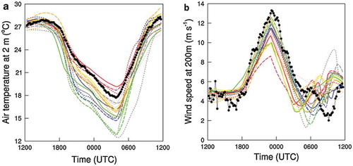
The Hu, Nielsen-Gammon, and Zhang (2010) and Hanna et al. (2010) results were also based on using the same land surface scheme (the NOAH scheme – Ek et al. 2003). Difference in land use schemes can have a major impact on model behavior (see section 5 below). The international GEWEX Atmosphere Boundary Layer Study (GABLS) group carried out a comprehensive study of boundary layer performance for a variety of PBL schemes and land surface models (see Bosveld et al. 2014). Figure 1 from that study provides a diurnal cycle for the test period for air temperature at 2 m and 200 m wind speed. The different models are shown in different line colors and patterns. Observations are shown as black dots. The figure shows that while different models have smaller spreads in wind speed and temperature in the daytime boundary layer, much larger spread (model uncertainty) exists in the nighttime stable boundary layer. Hence, below several topics address the stable boundary layer.

Figure 1. Comparison of the performance of different boundary layer and land surface models carried out under the GABLS program at a specific location for a 1-day period. Investigators from around the world were invited to carry out a specific experiment. The different colored lines represent different models. Panel (A) is the 2 m air temperature. Panel (B) is the wind speed at 200 m. Observations (black dots) are from Cabauw Experimental Site for Atmospheric Research (CESAR), the Netherlands (http://www.cesar-observatory.nl). At the Cabauw site midnight, local time is approximately 00UTC. Note that the widest spread occurs in the nighttime boundary layer. Adapted from Bosveld et al. (2014). See Bosveld et al. (2014) for details.

Turbulent mixing in the stable boundary layer

In the 1970s and 1980s, models began using local mixing schemes (e.g. Blackadar 1979; Mellor and Yamada 1982) for the stable boundary layer and employed turbulent kinetic energy models or stability function closures based on Monin-Obukov similarity functions (Businger 1973). With these new closures (though more physically based), models began to have a problem of becoming too stable, producing a boundary layer with surface conditions becoming too cold and calm (Shir and Bornstein 1977; Zdundowski, Henderson, and Hales 1967). Mixing of heat and momentum (or ozone) to the surface was too strongly suppressed (Beljaars and Holtslag 1991; McNider et al. 2012; Viterbo and Beljaars 1995). In these coarse grid models of the time, it appeared that additional mixing was needed (Savijärvi 2009). This was often implemented by using longer-tailed stability functions (see below) which had more mixing at stronger stability (in turbulent mixing schemes).

In K closure models in the stable boundary, the vertical mixing is often parameterized (Blackadar 1979; Savijärvi 2009) by

(1) $K=f(Ri)l^{2}s,$(1)

where Ri is the local gradient Richardson Number, l is a mixing length, s is the local shear and f(Ri) is the stability function. Figure 2 shows the stability functions used or discussed in the present paper. The longer tailed functions are those that maintain mixing beyond a critical Ri of about 0.25. The England McNider quadratic form was found by analytically solving for the stability function using Monin-Obukov similarity (see England and McNider 1995 for the analytical details). The Pleim Polynomial (see Pleim et al. 2016) was based on fits to a database of 80 LES simulations (Esau and Byrkjedal 2007), and then tested against GABLS-GWEX inter-comparisons. Both the England and McNider and the Pleim Polynomial, based on theory and observations, would be considered short-tailed because they cut off turbulence at Ri~.25. The Beljaars and Holtslag (1991) and Louis (1979) would be considered longer tailed forms. They were developed to add mixing into models that tended to have surface temperatures too cold and too calm in stable boundary layer. The long-tailed forms represented empirical adjustments to improve model performance in more coarse gridded models.

Figure 2. Stability function f(Ri) forms for the stable boundary layer used in Figure 1 or mentioned in the present paper (England–McNider – England and McNider (1995); Pleim ACM2 Polynomial – Pleim (2007a, 2007b); Beljaars-Holtslag – Beljaars and Holtslag (1991); Louis – Louis (1979); and Poulos et al. (2002)). From McNider et al. (2018).

In the 15–20 years since, the inadequate turbulent mixing began to be addressed (by adding mixing). It now appeared that with increased vertical resolution and/or improved radiation schemes, some models were making the opposite error, now having too much mixing (McNider et al., 2012; Steeneveld et al. 2008a; Savijärvi 2009). Savijärvi (2009) summarizes the issue very well; that models at higher resolution with the longer tailed forms had too much mixing, resulting in temperature and wind over-prediction, especially over oceans and homogeneous settings. This was also seen in air pollution studies (Garcia‐Menendez, Hu, and Odman 2013; Ngan et al. 2013; Lee et al. 2014), with too much downward mixing of heat, momentum and ozone from aloft at night.

The modifications to models to increase turbulent vertical mixing discussed above went beyond adjusting stability functions. Other adjustments, such as making the critical Richardson Number (bulk or gradient) a function of grid spacing (McNider and Pielke 1981; Panofsky and Prasad 1965), setting minimum values for vertical eddy diffusivities (Appel et al. 2007; Pleim, 2007a, 2007b), or setting minimum values of surface friction velocity were employed. Shir and Bornstein (1977) also explicitly addressed the model resolution in calculating Ri, pointing to the need for Ri_c to be dependent on grid spacing (Panofsky and Prasad 1965) or values of K’s increased (Neumann and Mahrer 1971). Not all boundary layer schemes (at least employed at high resolution) seem to have a warm bias. The results in Hu, Nielsen-Gammon, and Zhang (2010), discussed above, in which nighttime temperatures were too cold, are perhaps consistent because the Pleim ACM2 and the MYJ schemes are short-tailed forms. In summary, the SBL remains a challenge for modelers. A major problem may be the vertical resolution required to model very stable boundary layers. Sometimes at very small Monin-Obukov lengths (L < 10), the boundary layer height may not be captured in a coarse grid model (see McNider et al. 2012). Even if the resolution in the very lowest layers is adequate, resolving the height of the boundary layer top can be an issue if model resolution becomes coarser as model height increases. In addition, since mechanical mixing plays a major role in nighttime model performance, land use and associated roughness may play a key role in model performance. At present, roughness is highly parameterized from land use characteristics. Full variation in roughness due to urbanization may not be handled well in models. Nielsen-Gammon et al. (2010) developed a technique to carry out estimation of parameters in boundary layer schemes to improve model performance.

Given the uncertainty in modeling of the SBL, perhaps there should be consideration of confidence in regional meteorological and air quality models for regulatory actions where nighttime performance influences performance. As nitrogen emissions have been reduced, less nighttime titration may maintain higher surface ozone (Howard and Bacon 2014). Eighthour design values may include a greater number of nighttime hours. Perhaps a community review is needed, such as the review of point source models that led to the current AERMOD system (Cimorelli et al. 2005), to determine whether the uncertainty in modeling the SBL may undercut control strategy plans.

Wind speed bias

As noted in Jiménez and Dudhia (2012) the WRF model has had a high surface (10 m) wind speed bias over land since the early versions of the model (Cheng and Steenburgh 2005). This is consistent with bias discussed by Seaman (2000) and Hanna and Yang (2001). The bias persists in more recent versions (Mass and Ovens 2010, 2011; Roux et al. 2009). Wyszogrodzki et al. (2013), in a 15-month evaluation period (June 2009 – September 2010) of 4 km CONUS WRF simulation, found surface wind speed is strongly positively biased at night during the entire study period, with the averaged biases ranging between 0.5 and 1.0 m s⁻¹, and peaks up to 2 m s⁻¹ at times.

The solution proposed in Jiménez and Dudhia (2012) and by Mass and Ovens (2010) was to add a topographic drag term. Mass and Owens adjusted the friction velocity (u_*), while Jimenez and Dudhia added a separate momentum sink. Steeneveld et al. (2008b) also proposed a terrain drag. However, there may be some inconsistency in simply increasing u_*, since larger u_* in the stable boundary would increase mixing of downward momentum (and heat). While these adjustments appear to improve the model performance, it also may be pointing out uncertainty in model parameterization especially in the SBL.

The high wind speed bias in wind speed is of particular concern in air quality modeling. If the wind speed bias is not just a surface error, but extends through the boundary layer, this can lead to effective errors in ventilation and produce what may appear to be a bias in emissions. It seems that issues with the stable boundary layer and high wind speed bias for air quality models is a continuing concern and related to both the choice of the PBL scheme and model vertical resolution.

Extremely stable conditions

Extremely light winds and clear skies can lead to very stable conditions with boundary layer heights less than 10 m, which is often below the first model level in gridded models used in air quality studies. Plume models such as AERMOD (Cimorelli et al. 2005) face similar issues with defining plume behavior for shallow boundary layers. McNider et al. (2012), in a stable boundary layer climate impact study, used a 2-m vertical model resolution in a 1-D modeling study. This was to capture these extremely stable conditions. McNider et al. (2012) used special numerical techniques to avoid numerical diffusion that can overwhelm the physical SBL in light wind conditions. However, such strategies in gridded air quality modeling where horizontal grid scales are usually greater than 1 km can miss land use variations, which have a large impact on SBL turbulence and temperatures (Runnalls and Oke 2006).

Re-diagnosis of mixing coefficients

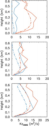
In offline air quality models such as the traditional CMAQ (Byun and Schere 2006) and CAMX (ENVIRON 2013), in which meteorological processes are concluded in advance of the chemistry model, turbulent mixing coefficients (K’s) may be recalculated from the meteorological data passed to the air quality model. In-line models such as WRFCHEM (Grell et al. 2005) avoid this step since meteorology and chemistry are calculated simultaneously. In the past, one of the concerns by modelers was how often should meteorological variables be passed to the chemistry model. This was based on the fact that meteorological variables may reflect the result of mixing, not mixing itself. If they are passed every time step, the storage and speed of the simulation may be a major issue. Many models such as CMAQ have used an hour time scale as a viable period. However, in a recent study (McNider et al. 2018) an additional problem was found when the vertical turbulent mixing coefficients (K_z for heat, momentum and scalars) formulations used in the meteorological model were different than in the chemistry model. In this study, which was examining mixing in the summertime stable boundary layer over Lake Michigan, a CMAQ mixing sensitivity run was designed to test the impact of mixing on surface ozone. Cleary et al. (2015) showed that the NOAA operational CMAQ model produced ozone levels that were higher than that observed by ferry on summer transects across Lake Michigan. A sensitivity study was carried out to examine the potential cause for this over-prediction by the model. A WRF base case simulation (for small mixing) was performed using the Pleim Polynomial/ACM2 stability function (see Figure 2). A second WRF simulation was configured to have enhanced mixing using the Louis stability function (see Figure 2) compared to the ACM2 scheme. The runs included the standard differences in mixing coefficients for heat, scalars and momentum based on the Prandtl Number included in CMAQ. Note that the K’s discussed herein are vertical mixing coefficients (see equation 1) and are a model heuristic not an observed quantity. These model configurations were then used to make two July 2011 WRF simulations. Subsequently, the output from the two WRF runs were used to drive two CMAQ simulations. The CMAQ uses the ACM2 formulation internally to re-diagnose mixing coefficients. The turbulent vertical mixing coefficients from CMAQ were then examined. Figure 3 shows that, in fact, the vertical mixing coefficients from the WRF/Louis case (enhanced mixing) were actually less than the vertical mixing coefficients in CMAQ driven by the WRF/ACM2 which had less mixing. As discussed in McNider et al. (2018), this occurs because WRF with the Louis scheme has already mixed out the shear, which is needed to produce turbulence in the ACM2 re-diagnosis. Future modelers should be wary of this issue. It is recommended as a minimum that WRF be used with the same mixing scheme employed in CMAQ. However, even here the use of offline meteorology (re-diagnosing mixing coefficients) can possibly lead to differences in the mixing in the stable boundary layer. This is because the wind and temperature profiles passed to CMAQ reflect past mixing, which may not be found in the re-diagnosed mixing coefficients. Thus, the preferred path would be to pass the mixing coefficients directly from WRF to CMAQ rather than having them re-diagnosed in CMAQ. Inline chemistry models such as WRF-Chem (Grell et al. 2005) do not have this potential problem.

Figure 3. Vertical profiles of mixing coefficients (K’s) diagnosed in CMAQ for the ACM2 and Louis WRF cases. The top panel is for the cross-section 1° latitude north of the ferry path described in Cleary et al. (2015) where ozone observations and models were compared. The middle panel is for cross-section near the ferry transect and the bottom panel is for cross-section 1° latitude south of the ferry transect. The solid lines are for the ACM2 case (small mixing) and dashed dotted lines for the Louis case (large mixing). Blue is for 12 UTC and red for 18 UTC. Note that the re-diagnosed K’s in CMAQ are consistently larger for the ACM2 case than the Louis case. Adapted from McNider et al. (2018).

Elevated polluted layers – mixing and advection above the planetary boundary layer

Most of the discussion above has highlighted the mixing in the stable boundary layer. However, as lidar measurements have become more prevalent, the role of mixing and advection above the PBL has become an issue in modeling. Some of the first lidar measurements of air pollution studies were carried out in Southern California (McElroy and Smith 1993; Wakimoto and McElroy 1986). They outlined previous studies of elevated polluted layers and mechanisms for their origin (see McKendry and Lundgren 2000 for a review). In these studies, they noted that mesoscale phenomena, variation in height of the marine inversion (McElroy and Smith 1991), return flows in sea breezes and topographic circulations (Wakimoto and McElroy 1986), and interaction of synoptic high-pressure systems with topographic and coastal geometry (Mass and Albright 1989) could lead to elevated pollution layers that might affect regional pollution. Model studies (Ueyoshi and Roads 1993; Ulrickson et al. 1995) explored the details of the synoptic and mesoscale development of the Catalina Eddy and the role these situations play in elevated polluted areas.

Layering can also develop due to the physics of entrainment and reductions in the PBL depth during the day. In the growing PBL, overshooting of thermals or shallow cumulus can allow surface precursors, such as VOCs and NO_x, to be trapped just above the fully turbulent boundary layer (Fast and Berkowitz 1996; Vukovich, Fishman, and Browell 1985). Here, high photolysis levels and lack of deposition losses can increase ozone and fine particle concentrations (Gregory, Browell, and Warren 1988).

In the intervening years, lidar observations of both aerosols and ozone have shown the existence of elevated polluted layer across the U.S. and the world (Kovalev et al. 2009). As traditional emissions have been reduced, greater attention has been given to wildfires and prescribed burns in influencing air quality. Lidar and satellites have quantified many of these free troposphere events (Kovalev et al. 2009; Nepomuceno Pereira et al. 2014). Multi-sensor and field studies have allowed the impact on local air quality to be determined (Gupta et al. 2018; McKendry et al. 2011; Reid et al. 2017). These lidar measurements can also provide another path for evaluating models in the free troposphere (Wang et al. 2017).

Regional and mesoscale structure important to air quality

Most major urban areas, because of transportation, water needs and building considerations are located in valleys or along bodies of water. As discussed by Pielke et al. (1991), topography and land/water temperature contrasts can produce mesoscale flows that can alter air quality potential and locations of air quality impacts. The gridded models in use today, such as WRF, have the physics and small grids needed to resolve these mesoscale circulations. The following reviews these mesoscale flows and model configurations needed to capture the circulations.

Topographic/flows and valley stagnation

Heated and cooled sloping terrain can produce upslope and drainage flows as well as thermal mountain and valley flows that direct flows not just up and downslope but also up and down the direction of a valley (McNider and Pielke 1984; Tyson and Preston-Whyte 1972). Whiteman (1990) and Whiteman (2000) provide extensive reviews of topographic flows, especially thermally driven systems with an emphasis on observations in complex terrain. Zardi and Whiteman (2013) provide a review of observations and modeling of topographic flows. Fast (1995) also showed that shear in drainage flows can have a major impact on plume behavior and suggested that turbulent parameterization may have an important role in plume spread and concentrations (see also Seaman 2000). However, wind shear in these flows can significantly impact plume concentrations (McNider, Moran, and Pielke 1988). Topography can also produce channeling of flows. Since the topography is fixed, there might be preferred directions of flow that can alter the location of air quality impacts.

Stagnation in valleys can also be an issue in air quality, especially for particle loading in populated western valleys during the winter, such as the Salt Lake Basin or San Joaquin Valley (Baker, Simon, and Kelly 2011). Since slight turbulent fluctuations continue to exist even under light wind conditions, stagnation may be defined when the turbulent fluctuations exceed the mean wind. Whiteman, Bian, and Zhong (1999) discussed many aspects of valley stagnation over the Colorado Plateau Basin, including the formation, maintenance and dissipation of valley inversions. As noted by Baker, Simon, and Kelly (2011), routine application of prognostic meteorological models, including the Fifth-Generation NCAR/Penn State Mesoscale Model (MM5) and Weather Research and Forecasting Model (WRF), with a variety of different physics options, vertical and horizontal resolutions, and nudging approaches have failed to replicate the degree and persistence of stagnant meteorological condition (Zhong et al. 2001). However, as discussed in Seaman et al. (2012) for an eastern valley, extremely high vertical resolution (11 model layers below 50 m compared to 4 layers below 50 m) may be required to properly capture the physics and mixing of the stable conditions. The stable boundary layer may require very fine vertical resolution less than 8 m near the surface (Shir and Bornstein 1977) to capture gradients in Richardson number closures or TKE closures (Blackadar 1979; Mellor and Yamada 1982).

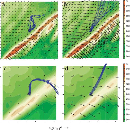
As discussed by Seaman et al. (2012), small-scale topography and fine scale vertical resolution is also needed to resolve gravity waves and drainage flows which contribute to mixing in nighttime boundary layers in valleys. Mixing and fine scale flows can make large differences in pollutant trajectories and horizontal mixing. Seaman et al. (2012) performed four experiments varying horizontal and vertical model resolution. The Baseline Experiment was at fine horizontal resolution (0.444 km) and fine vertical resolution (first model level at 2 m). A coarse vertical resolution case with first layer at 33 m and horizontal resolution at 0.444-km was denoted LargeDZ. A coarse horizontal resolution experiment (1.33 km) with fine vertical resolution (first level at 2 m) was denoted as LargeDX. Finally, a coarse horizontal resolution (1.33 km) and coarse vertical resolution (first level 33 m) experiment was denoted LargeDXDZ. Figure 4 shows the model domains for the model set up in the Nittany Valley of Pennsylvania near the town of Rock Springs. Simulations were carried out for 7 Oct 2007. The figure provides an example of the differences in wind and trajectories for the four different model vertical and horizontal resolutions. As shown in the figure, the direction of the trajectories can depend on both vertical and horizontal resolution. It was also noted that gravity waves and mesoscale oscillations supported by the fine scale terrain could alter the spectral character of the winds affecting turbulence and meandering.

Figure 4. Predicted parcel trajectories at 0800–1112 UTC (blue) and wind vectors at every other grid point at 1112 UTC at the lowest model level in a sub-region in the vicinity of Rock Springs, Pennsylvania in the Nittany Valley on 7 Oct 2007. Nine parcels were released at 3 m AGL in a 0.444 km x 0.444 km area denoted by the inverted triangle at 0800 UTC. Results are for (A) Baseline Experiment Fine vertical and horizontal resolution, (B) Large DZ Experiment, (C) Large DX Experiment, and (D) Large DXDZ Experiment. Terrain (m) is shown as color fill. The distance scale can be seen in the spacing of the wind vectors (0.888 km). From Seaman et al. (2012).

Sea and lake structures

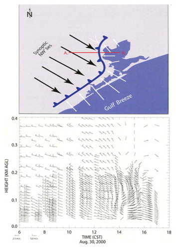
Land water contrasts and resulting thermal circulations that are not resolved synoptically have long been a factor in pollution in coastal cities (Bornstein and Thompson 1981 for New York; Keen and Lyons 1978 for Chicago; Banta et al. 2005 for Houston). The long standing and continual problem for Los Angeles air quality is tied both to sea/land breezes in the area (Lu and Turco 1995) and mesoscale features such as the Catalina Eddy (Mass and Albright 1989). Bornstein and Thompson (1981) and Banta et al. (2005) emphasized the role of the developing sea breeze in reducing ventilation over source regions. Figure 5 from Banta et al. (2005) shows a schematic of how an opposing synoptic flow can inhibit the movement of the sea breeze front. With the sea breeze stalled, it can produce light winds over pollutant source regions. This can lead to accumulation of precursors, leading to bands of high ozone concentrations later in the day as the sea breeze moves inland. A similar phenomenon occurs in Los Angeles as high levels of precursors and ozone are carried inland to places like Riverside.

Figure 5. (top) Schematic of stalled sea breeze in Houston due to opposing synoptic winds. (bottom) Time-height cross-section of Doppler observed winds at La Porte showing light winds and potential precursor accumulation in sea breeze front. From Banta et al. (2005).

More recent papers in the literature supported by new observations and modeling, have discussed the role of over-water stability affecting ozone levels. Goldberg et al. (2017) noted that higher overwater ozone concentrations (over the Chesapeake Bay) are supported by (1) shallower boundary layers trapping shipping emissions near the surface, (2) higher photolysis rates due to clear skies over the bay, (3) decreased boundary layer venting due to a lack of fair-weather cumulus clouds, and (4) slower deposition losses over water. Loughner et al. (2014) discussed the important role of model resolution in capturing elements of the over-water ozone behavior. For the Chesapeake Bay, a 1.33 km horizontal mesh was needed to capture the structure.

High levels of ozone along the shores of Lake Michigan have been a continuing problem for air quality agencies in the region for nearly 40 years (Cleary et al. 2015; Foley et al. 2011; Lyons and Cole 1976). Keen and Lyons (1978) described the characteristics of the Lake Michigan sea breeze in light of traditional conceptual models of lake breeze systems with an emphasis on the onshore convergence lines which can transport pollutants aloft into the offshore return circulation. Levy et al. (2010) provided a comprehensive list of the physical-related factors, which impact local lake and land breeze circulations such as shoreline curvature, urban land use and synoptic settings. Lyons and Cole (1976) discussed the impact of the thermal destruction of the lake-breeze flow as it moves inland producing local high concentrations, as well as the long-range effects of combined recirculation and alongshore transport of urban and power plant plumes.

Over the lake, a shallow but steep stable layer is maintained through most of the ozone season due to cold lake temperatures. While intimated in early conceptual models of the Lake Michigan lake breeze systems (Lyons and Cole 1976), aircraft measurements (Dye et al. 1995; Foley et al. 2011) have verified high levels of ozone aloft over the lake. Dye et al. (1995) characterized the lake breeze as a near perfect reaction chamber with precursors imported from the urban areas, large photolysis rates due to clear skies in the subsidence zones over the lake and a lack of surface losses from deposition or NOx titration (Angevine et al. 2004). The high ozone in this reaction chamber can then be brought back to shore, although often translated alongshore, creating high coastal ozone (Angevine et al. 2004). McNider et al. (2018) showed that issues with re-diagnosing mixing coefficients (see above) in the overwater stable boundary layer may be the cause of operational CMAQ over-water over prediction of ozone (Cleary et al. 2015).

Low-level jet

While the above topographic and land/water contrast focused on spatial mesoscale structure, the low-level jet represents a temporal mesoscale feature that can be a dominant factor in sustained plume growth rates and export of pollutants from urban areas during light synoptic wind cases (Chen, An, and Sun et al. 2018; McNider, Moran, and Pielke 1988).

As discussed first by Blackadar (1957), the low-level jet develops overnight under conditions of clear skies and relatively light geostrophic winds, where a stable boundary layer can develop (note these are often conditions for air pollution episodes). As the nighttime boundary layer stabilizes, momentum fluxes to the surface are reduced. Thus, the layer of air above the shallow nocturnal boundary layer reduces friction and begins to accelerate. As the air accelerates, Coriolis forces turn the unbalanced winds, leading to an inertial oscillation as the layer seeks a new geostrophic balance. Thus, an evolving low-level jet is a persistent part of the nocturnal boundary layer.

Figure 6A shows a time sequence of the modeled Houston ship channel plume during the 2000 Texas Air Quality Study (TEXAQS-2000). The Lagrangian Particle Model (LPM) is that described in McNider, Moran, and Pielke (1988), in which particles are moved with both the mean wind and turbulent fluctuations. The horizontal turbulent fluctuations (σ_v, σ_u) and Lagrangian timescales are diagnosed from the model boundary layer parameters (Hanna 1983). Vertical turbulent fluctuations are recovered from the vertical mixing coefficients based on techniques described by Hanna (1968). It shows that during the day winds were light with a modest sea breeze carrying the urban plume slowly to the northwest. What is remarkable is how little the plume moves during the day and how little horizontal dispersion takes place. The boundary layer to the north of the Gulf in Houston is convective during the day with little vertical shear. Here, the horizontal spread is limited to primarily convective turbulence and scales. Using Taylor’s theorem (see Hanna, Briggs, and Hosker 1982) one can estimate this convective spreading using a σ_v ~2.0 m/s and a Lagrangian time scale ~ 500 s and a daytime travel time of 10 h. This yields a plume σ_y of about 10–12 km or a total width of about 20 km. The width of the plume in Figure 6 is about 30 km at sunset, but some growth is due to boundary layer shear. So the growth until about sunset is consistent with boundary layer theory.

Figure 6. (A) Depiction of a modeled continuous plume release from near the Houston ship channel with release beginning in the early morning. Note that in left panel (00UTC) after 10 h of the release, the plume has not traveled far nor spread very much (about 30-40 km wide). But in the next 6 h (middle panel) as the inertial oscillation begins, the plume travels and spreads rapidly. By early the next morning, the plume has spread over much of east Texas. Colors indicate height of particle in km. From an operational run providing support to TEXAQS 2000. (B) Depiction of transport and spread for point source plumes for a Northeast simulation reported by Zhang and Rao (1999). Note spread and shape is consistent with the LLJ spread in (A).

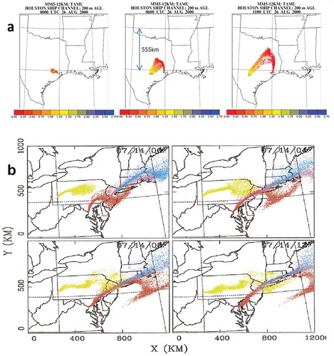
However, near sunset, the daytime convective boundary layer collapses. This leads to the Blackadar inertial oscillation. The acceleration creates strong winds and strong shear that rapidly transports and distorts the urban plume. However, this distortion is not diffusion. By early morning, the next day, the urban plume has been sheared across most of East Texas. As the boundary layer develops the next day, the distorted plume is then diffused over a large horizontal area. Thus, not only has the inertial oscillation exported ozone and precursors out of the urban area, it has partially defined the regional background impacting San Antonio, Austin and Dallas. In addition to this effect, as the rotating inertial oscillation continues into the next morning, it creates a wind opposing the development of the local sea breeze. This can then lead to stagnation over source regions south of the city as discussed above (Banta et al. 2005) leading to high concentrations of precursors. Zhang and Rao (1999) using a one-dimensional (1-D) model and a Lagrangian particle model also showed similar geometry of plumes (see Figure 6B) over the Northeast U.S. The 1-D model described by Zhang and Rao (1999) had the requisite physics to produce the LLJ. The pattern seen in Figure 6B is consistent with the LLJ, but they did not explicitly discuss the role of the LLJ.

In the early 1980s, there was debate (Gifford 1982, 1983; Smith 1983) on why long-range measurements of Australian smelter plumes continued to grow horizontally at rates much faster than turbulent theory. Gifford (1983) argued that the growth was maintained by mesoscale spatial turbulence with scales larger than the plume. Smith (1983) argued that shear was responsible for maintaining the plume growth. McNider, Moran, and Pielke (1988) showed that the Blackadar inertial oscillation produced shear leading to a much wider plume the next day. Near sunset (18 LST), as the inertial oscillation begins, it starts to distort the plume so that by about 03 LST the plume is elongated. At this stage, there has been no actual diffusion (change in local concentrations) only distortion. Nevertheless, when the next day’s boundary layer begins to grow (about 09 LST), vertical mixing produces a much wider plume than would be produced by turbulence alone. Plume widths are often 10–15 times that without the inertial oscillation. McNider, Moran, and Pielke (1988) noted that this shear was the result of temporal mesoscale motion (the inertial oscillation), so both Gifford and Smith were partially correct. This is the process for the extremely wide Houston ship channel plume seen in Figure 6A and for the plumes seen in Figure 6B.

Bonner and Paegle (1970) showed that a combination of changes in the topographic driven pressure gradients and change in friction leads to larger Blackadar inertial oscillations by 20-50% over the Great Plains and in coastal areas (McNider, Mizzi, and Pielke 1982; McNider and Pielke 1981). The low-level jet is strong when the evolving thermal gradients over the large scale heated sloping terrain or in coastal areas reinforce the geostrophic wind. The impact of data assimilation on modeling the inertial oscillation is discussed in the next section.

Synoptic scale structure important to air quality

Large-scale weather systems have long been related to air pollution potential because the physical parameters discussed in the introduction – temperature, winds, humidity and sunlight vary greatly across the highs, lows and fronts, making up the large-scale weather. The following discusses the large-scale weather that can lead to high air pollutant potential and impact the mesoscale and turbulent structures discussed above. Paths and techniques to include the large-scale weather are reviewed. Also, see Seaman (2000) for another review perspective.

Synoptic settings conducive to high concentrations

Traditional conceptual models of synoptic conditions conducive to high concentrations of air pollutants have focused on the center of slow-moving high-pressure systems (Stern 1984). Here, light winds and short trajectories reduce dilution. The southeastern side of the high-pressure system also produces subsidence through the conservation of potential vorticity, leading to reduced mixing heights and decreased cloudiness (Holton 1973). Thus, the center of high-pressure system produces low ventilation (Altshuiler 1978; Holzworth 1972) reduces mixing heights, and has high photochemical potential.

However, in the study of the regional meteorological conditions associated with high ozone concentrations in the Southeast under the Southern Oxidant Study (SOS) (see Solomon, Cowling, and Weber 2003), it was found that a majority of the extreme events (regulatory design days) occurred in association with stationary frontal zones or trough lines (McNider et al. 1995). Later, as SOS moved into Texas, it was found that extreme events (8-h design periods), especially in Dallas, were also tied to stationary fronts. In fact, during 1999 all of the highest 8-h ozone values in the Dallas were associated with stationary fronts. An analysis was made of all these events (McNider et al. 2005). The August 2–5, 1999 was typical of these stationary front events. As a cold front stalled over North Texas, ozone in the Dallas area deteriorated over several days. Figure 7 shows an example of high ozone near Dallas in the presence of the stationary front and a model depiction of winds.

Figure 7. The Dallas ozone event discussed in the text evolved over several days – August 2–5. (left) Depiction of ozone observations in East Texas at 14:00 LST August 3– 4 1999 and the analyzed stationary front position. (Right) MM5 model depiction of surface winds for August 3–4, 1999. Wind vector length provides relative wind speeds. Wind speeds (m/s) are color coded. Figure adapted from McNider et al. (2005).

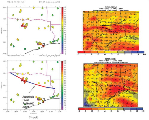
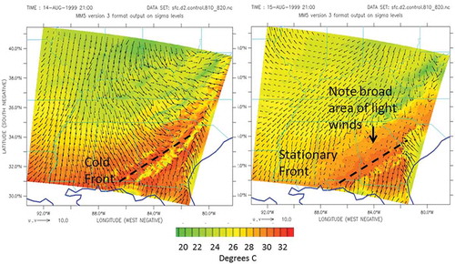
Since cold fronts can be associated with cloudiness and deep mixing and warm fronts with cloudiness, there was some perplexity by researchers of the cause of the high ozone. Studies, including aircraft investigations, were carried out over several years by SOS and Texas investigators to examine why stationary fronts might be conducive to high concentrations. Modeling studies indicated that light winds in and near the actual front lead to a zone of poor dilution, leading to a buildup of precursors and ultimately ozone. By the very nature of opposing flows on either side of the stationary frontal zones, winds by necessity must go to zero across the front. As the cold front stalls, this area of light winds broadens. Figure 8 shows the evolution of a cold frontal transition to a stationary front. It can be seen that as the front stalls, a broad area of light winds develops. As seen in the figure, this produces higher temperatures as mixing and ventilation are reduced near the front. This is in part due to relatively low levels of cloudiness north of the front. As the front stalls, the flow regime transitions from a convergent flow pattern to a deformed flow pattern (see Hess 1959). In a deformed flow pattern, there is little convergence to provide lifting and cloud formation. Thus, heating and photochemical production can be high. Additionally, in examining two-dimensional cross-sections through a front, it was deduced that the sloping frontal inversion extending to the north side of the front inhibits boundary layer growth. This caps pollutants in a relatively shallow boundary layer. Finally, the very nature of a stationary front means that movement of the front back and forth can lead to short and even circular trajectories leading to a buildup of ozone.

Figure 8. MM5 modeled evolution of a cold front to a stationary front in South Georgia August 14–15,1999. High ozone levels (above hourly values above 35 ppm) occurred in Macon, Georgia during this period. The left panel shows substantial winds from the northwest pushing front south. The right panel shows the flow is now more parallel to front leading to a stationary front. Winds are light in a broad area north of the front as it becomes stationary. Notice that higher temperatures north of frontal zone associated with light winds and clear skies. Temperatures are color coded on right legend.

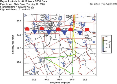
Because of the importance of stationary fronts to regulatory design periods, special aircraft measurements were made across stationary front as part of the TEXAQS 2006 (McNider et al. 2008). Figure 9 shows a horizontal plot of aircraft observed ozone. Measurements indicated that precursors and ozone increased in the area north of the front confirming the stationary front hypotheses mentioned previously.

Figure 9. Depiction of Baylor aircraft measurement of ozone across a stationary front near Dallas on August 22, 2006. It shows that ozone is highest just north of the front. Aircraft wind speeds also dropped by a couple of meters/sec crossing the front. Adapted from McNider et al. (2008).

Modeling of design periods of stationary fronts for regulatory actions has been problematic. Modeling systems such as MM5 and WRF can capture the characteristics (low wind speeds, high temperatures, frontal inversion capping) that lead to high concentrations. However, the ability for the large-scale initialization to locate the position of front accurately is difficult. This is in part because analyses, using rawinsonde data (in four-dimensional data assimilation) are often too coarse to identify the location of the front. Even small position changes in the front can alter spatial ozone levels.

Including large-scale structure – use of four-dimensional data assimilation

Initially, large-scale meteorology was incorporated through initial conditions on the fine-scale model grid and updated through boundary conditions for the forecast period in the same way finer scale weather forecast models are run. As noted in the introduction, for many regulatory actions, air quality models are used in a retrospective mode, attempting to recreate past air quality episodes. This provides an opportunity to use observed data (surface, upper air and special observations) to improve model performance. Meteorological models run at high-resolution need to assimilate largescale (synoptic) observations to avoid forecast drift (Stauffer and Seaman 1990, 1994; Stauffer, Seaman, and Binkowski 1991; Shafran, Seaman, and Gayno 2000) and yet not degrade the mesoscale structure and local boundary layer characteristics important to air quality simulations (Appel 2014; Shafran, Seaman, and Gayno 2000). However, data assimilation can also include observations that capture scales not resolved in the grid models (Barna and Lamb 2000; Scire, Insley, and Yamartino 1990; Umeda and Martien 2002).

Two different major approaches covered under the name of Four-Dimensional Data Assimilation (FDDA) have been used. See Seaman (2000) for a detailed review. The first approach, which has been incorporated largely by the weather forecast community, is variational analyses. Here, using mathematical optimization techniques, the model field is minimally adjusted to agree with an observational analysis. Today, this includes both three-dimensional (spatial −3DVAR) variation (Kalnay 2003) as well as four-dimensional variation (including time −4DVAR) to adjust the model field. However, as discussed by Seaman (2000), in the air quality community FDDA has largely been based on Newtonian relaxation nudging (Hoke and Anthes 1976; Stauffer and Seaman 1990). Here, model variables are nudged over time to agree either with point observations using a radius of influence or with an analysis field. Early FDDA strategies (Stauffer and Seaman 1990) employed a nudging coefficient on the order of the Coriolis force (10⁻⁴s⁻¹) to capture the synoptic scale features but not to significantly dampen the mesoscale structure.

Umeda and Martien (2002) employed a different technique that included spatial and temporal nudging weights. This provided larger nudging near the boundaries but less in the interior where it was felt model-resolved mesoscale structure should be maintained. Stauffer and Bao (1993) also described a technique which developed nudging coefficients that minimized error. They indicated it showed promise but was sensitive to minimization penalties.

While nudging generally improved model performance (Otte 2008), there is still concern that nudging to the large-scale analysis may adversely impact mesoscale structures important to air quality not resolved in the analysis. A study by Appel (2014) used an iterative FDDA technique in which an initial large-scale analysis used in the FDDA nudging is replaced by a second nudging field produced by the initial fine scale simulation. The Appel (2014) study was trying to capture the fine-scale details of the Chesapeake Bay area.

Appel (2014) noted that the use of the larger-scale analyses produced a poor model performance for finer scale simulations (4-km and 1-km). In addition, soil moisture and temperature data assimilation were ineffective at the finer scales due to the inconsistencies of the NAM-12 analysis with the higher resolution geography, terrain, land use and soil data. In their iterative approach, the outputs from the initial finer scale simulations (4-km and 1-km) are used in the FDDA nudging instead of the NAM-12 analyses to produce a second iteration of WRF simulations. Observations are fused in the first iteration’s outputs to reduce the errors. This approach produced significant improvements in representing the temperature gradients in the Chesapeake Bay area (Appel 2014). However, a recent application of the Appel et al. iterative technique to the Lake Michigan area (Odman et al. 2019) did not show a significant improvement. This may be due to the presence of significant mesoscale topography and the complexity of the Chesapeake Bay land water boundaries compared to the Lake Michigan setting.

Alternate FDDA approaches

While Newtonian nudging has received the most usage and attention in air quality applications, there are new approaches that include and sometimes combine variational techniques (Huang 2009; Kalnay 2003), Extended Kalman Filtering (EKE- Wang et al., 2008a, 2008b), and Ensemble Kalman filtering (EnKF – Lei, Stauffer, and Deng 2012). White (2018) in an air quality study provided background on each of these techniques. Seaman (2000) also discussed these alternative approaches.

FDDA impact of modeling of the inertial oscillation

While an earlier section provided an understanding of the inertial oscillation and its role in air pollutant transport and dilution, the real issue today for regulators is how well physical models such as WRF handle the geostrophic gradients and mixing which control the inertial oscillation. If the physical models do not adequately capture the inertial oscillation, this may bias control strategies toward more local control. Primitive equation models such as WRF include the basic geostrophic adjustment processes to produce inertial oscillations and low-level jets. However, the magnitude of the inertial oscillations depend on parametrized processes such as turbulent mixing schemes and land use characteristics. As noted above, the nighttime boundary layer is especially problematic. Additionally, nudging strategies in models can greatly impact the inertial oscillation and the low-level jet. The case in Figure 6A for Houston was a free forecast run and did not include FDDA. Mass and Ovens (2010, 2011) as well as Jiménez and Dudhia (2012) also discuss a continuing problem of over prediction of surface winds especially at night that exists in most versions of WRF. Ngan et al. (2013), Lee et al. (2014), and Qin et al. (2019), in air pollution studies found over prediction at the surface at night but not aloft. However, Hu et al. (2012) for Maryland, Storm et al. (2008) for Central Texas, and McNider et al. (2017) for Houston showed inertial oscillation winds were underestimated in models.

As noted above, the inertial oscillation is a mesoscale temporal feature. There are also terrain effects/land use effects that are not resolved in coarse grid studies (see above the discussion in Seaman et al. 2012). Evaluating model winds is difficult using traditional paired in space and time statistics, in that transient wave motions with frequencies ½ hour to several hours can produce offsets in speeds and directions that can impact paired in space and time statistics. To avoid this issue, Gupta et al. (1997) developed a unique Fourier analysis technique, which evaluates how well the model captures particular wave periods as a function of height. Figure 10 shows an example of this technique for the Nashville SOS 1995 intensive. The inertial oscillation period for Nashville is close to the diurnal period. The figure shows that most of the wind energy is at synoptic time periods (4–5 days or 96–120 h) and models do a good job at capturing the synoptic motions in that the peak and shape of the model and observed spectra agree. However, the observed radar profiler data show that there is much greater energy in the inertial/diurnal wave periods than captured by the MM5 model (predecessor to WRF) for a simulation performed by EPA. In addition, there is perhaps unresolved energy at higher frequencies.

Figure 10. Comparison of spectral wind energy between observed wind profiler data and MM5 model spectra for Nashville 1995 simulations (see Gupta et al. (1997) for a description). The MM5 model was run by EPA and is different from the one-dimensional model used in Gupta 1997. The individual lines show the spectral intensities at a given height. Constants are added to the energy spectra amplitude at successive heights to separate them on the graph. The corresponding height of a spectrum can be read from the left axis. Note that model spectra on the left does a good job of replicating the synoptic scale energy (4–5 day or 96 to 120-h wave period) compared to the profiler observed on the right. As expected the synoptic spectral energy increases with height as synoptic waves have larger amplitude higher in the troposphere. But the model underestimates the diurnal/inertial period energy at the 24-h wave period compared to observations. As noted, this may be due to the nudging above the nocturnal boundary layer which is damping the diurnal/inertial energy. The noise above 2–3 km in the observation may be measurement error.

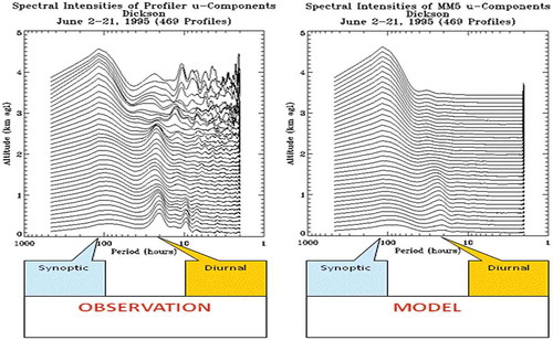
The smaller modeled energy at the inertial period may also be due to FDDA strategies such as mentioned above. Rawinsonde times (00UTC and 12UTC) in the U.S. Eastern and Central U.S. correspond roughly to sunset and sunrise. Thus, as described by Shafran, Seaman, and Gayno (2000) and Godowitch, Gilliam, and Rao (2011), rawinsondes are not likely to resolve low-level jets. In the absence of other data or model input to the analysis, the low-level jet may not be captured in the larger scale analysis. Thus, nudging to observational analyses may remove or reduce the strength of the low-level jet (Shafran, Seaman, and Gayno 2000; Zhang et al. 2001). The particular case in Figure 10 was based on the nudging strategy used by EPA at that time, in that nudging was carried out above the boundary layer. Gilliam, Godowitch, and Rao (2012) showed that because the nighttime boundary layer is so shallow, nudging can impact winds in the area where the LLJ develops.

To explicitly examine the impact of nudging strategies on the LLJ, a Lake Michigan centered WRF simulation was carried out for the month of June 2011. See Odman et al. (2019) for details. A simulation was carried out with nudging above the boundary layer and a second simulation where nudging was only applied above 2 km. Surface wind speed statistics were slightly improved when nudging was applied above the boundary layer compared to only nudging above 2 km.

Points were selected in the Midwest for locations where the NOAA operational profiler network had observations to examine the development of the low-level jet under both nudging strategies. Figure 11 shows that for the cases with no nudging in the boundary layer (but nudging above the boundary layer) the LLJ generally does not develop or is extremely weak. For the case where nudging is not applied below 2 km, a significant low-level jet develops. This illustrates the specific impact of FDDA in maintaining the LLJ. Odman et al. noted that a lower cutoff than 2 km might have been a better choice to maintain better winds between 1 and 2 km. Gilliam, Godowitch, and Rao (2012) in a comprehensive analysis of WRF model general wind performance, compared model to non-traditional profiler and radar winds. They showed that nudging above the boundary layer in the region of the low-level jet degraded model performance but did not emphasize the details of the jet under nudging strategies. Gilliam, Godowitch, and Rao (2012) also showed that assimilating the profiler and winds above the daytime convective boundary layer also improved wind performance in the convective boundary layer.

Figure 11. Model and observed wind profiles for a WRF model simulation around the Great Lakes for June 2011. The station identifiers are for the NOAA operational profiler network. (A) WNCI2 (Western Illinois) with left panel at 0300 UTC (2100 LST) 17 June 2011 and right panel at 0600 UTC (0000 LST) 4 July 2011, (B) WLCI3 (Northern Indiana) with left panel at 0400 UTC (2200 LST) 17 June 2011 and right panel at 0900 UTC (0300 LST) 24 July 2011, and (C) BLRW3 (Southwest Wisconsin) with left panel at 0400 UTC (2200 LST) 17 June 2011 and right panel at 1000 UTC (0400 LST) 29 June 2011. Black solid line is for nudging above PBL. Black-dashed line is for nudging only above 2 km. Blue solid lines are profiler observations. From Odman et al. (2019). The nocturnal boundary layer height is approximately just below the nose of the jet.

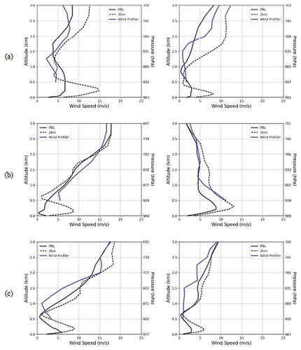
In Odman et al. (2019), in addition to the meteorological analysis, the CMAQ simulations were also performed for the two nudging cases to examine air quality impacts. The description of the CMAQ model configuration is given in Odman et al. (2019) and Qin et al. (2019). The emission scenario and CMAQ configuration were set as the same in the two nudging cases.

Figure 12 shows the difference in the ozone mean bias between the two model nudging cases. It shows that the case with nudging only above the 19th layer (~2 km) improves the model performance over much of the eastern U.S. and especially in the Midwest. Note the performance is especially improved along the periphery of Lake Michigan.

Figure 12. Change in ozone mean bias between the nudging above the boundary layer and nudging only above 2 km for the June 2011 case. Note improvement in the Midwest and around Lake Michigan from Odman et al. (2019).

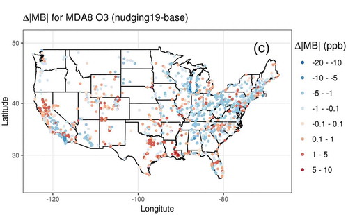
As noted above, the low-level jet appears to be a significant factor in exporting both ozone and precursors overnight out of source areas. But, is it an important issue for regulators? Models have consistently underestimated NO₂ column values in rural areas and overestimated NO₂ columns in urban areas compared to satellite column NO₂ (see Canty et al. 2015; Castellanos et al. 2011; Goldberg et al. 2017; Kuhlmann et al. 2015). Canty et al. (2015) concluded that the CMAQ model may underestimate the interstate transport of NO_x and/or NO reservoirs. Under-stating the LLJ, which may provide the main export of pollutants out urban under light winds (such as the Texas case above), would be consistent with this finding. Goldberg et al. (2017) found similar problems in CMAQ with under-estimates of rural NO₂ and over-estimates of urban NO_2. Goldberg et al. (2017) did not mention under-estimation of transport and attributed the problem to emissions and chemical mechanisms. However, the underestimate of transport in the model probably cannot be discounted.

More research is needed to understand the importance of the LLJ to these issues and impact on control strategies. We believe this is a component that should be of interest to the air quality research and regulatory community since it addresses a key model discrepancy issue. It may also impact background values in urban control strategy evaluations. Also, without the LLJ and export of ozone and precursors out of urban areas, it may make local emission reductions appear to be more effective than they may really be.

Land surface modeling and water surface specification

Land surface temperatures are largely controlled by solar energy input and the characteristics of the land surface, which partition outgoing energy into sensible and evaporative fluxes (Sellers et al. 1997; Wetzel, Atlas, and Woodward 1984) and to the thermal inertia of the land surface (Carlson 1986; McNider et al. 2005). Aside from its impact on temperature, the partitioning of solar energy into evaporative fluxes from vegetation is also critical for air quality since stomatal uptake of ozone is one of the major loss terms in the ozone budget (Pleim et al. 2001).

Because of the importance of the characteristics of the land surface, there has been tremendous investment by the climate, weather forecasting and air quality communities in land surface research. Much of this investment has gone into developing complex land-surface models, which include many intricate parameterizations that attempt to capture processes such as plant transpiration rates, leaf water interception, soil moisture and run-off, and parameterizations, which control thermal and water transfer through canopies and soils (Pitman 2003; Sellers et al. 1997). Thus, these models require additional parameter specifications to close the model systems.

The use of satellite data (with observations such as greenness and albedo) has greatly improved the classification of the surface. However, land surface models in WRF (Chen and Dudhia 2001) do not use land use classifications directly. Rather, they use physical parameters such as roughness, heat capacity, canopy thermal and water resistances, soil conductivity for water and heat, etc. that are associated with the land use classes. Thus, in models, such as the WRF-Noah land use model, there are lookup tables that define these land use associated parameters (Niu et al. 2011).

Unfortunately, the specification of some of these physical parameters is difficult even in homogeneous land use classes (Rosero et al. 2009). For example, the rate of temperature change in vegetation is controlled by plant transpiration and evaporation through water resistance parameters and by the canopy thermal resistance. Thermal resistance depends on the heat capacity of the canopy and the thermal conductivity through the canopy (Noilhan and Planton 1989). The water resistance depends on root zone moisture, the phenological state of the plant – leaf area, shaded leaf area, etc. Field campaigns using tower measurements are usually conducted to try to establish these parameters. However, in effect, many of the parameters or processes have to be deduced as residuals in local canopy models, which are tied to specific turbulence and radiative models (Pleim and Gilliam 2009; Yang and Friedl 2003). Thus, the parameters are often model heuristics (short-cuts to avoid complex calculations) as opposed to fundamental observables (Wagener and Gupta 2005), which is the reason a parameter such as canopy thermal resistance can vary by three orders of magnitude in different models (Pleim and Gilliam 2009). In inhomogeneous grid boxes, which make up the real world, the situation is even more difficult in terms of defining parameters (McNider et al. 2005).

The development of complex land-surface models mentioned above was consistent with the need in the climate modeling community for surface models that could be run for years without being influenced by observed data. Thus, they needed vegetative surface interaction, water balance models, etc. that could be run for long periods without being touched by data. However, Diak (1990), McNider et al. (1994), Anderson et al. (1997) and others argued that for short-term weather forecasting and for retrospective air quality simulations (McNider et al. 1998a; Pleim and Xiu 2003), simpler models that could be constrained by observations might be preferred. The simple models avoid setting many uncertain parameters in the complex models.

Pleim and Xiu (2003) recognized the uncertainty in soil moisture and developed an innovative technique that used the daytime differences between observed analyses and model values of 2-m temperatures and 2-m surface relative humidity to adjust soil moisture. Additionally, Pleim and Gilliam (2009) used nighttime differences between model and NWS observed data to adjust another non-observed parameter – deep soil temperature in the land surface scheme. These techniques have shown to improve model performance in both EPA studies (Gilliam and Pleim 2010) and external studies (Fovell 2013). Figure 13 shows examples of the impact of NWS assimilation and satellite assimilation (see below) into the Pleim-Xiu-Gilliam scheme during September 2013 for a domain centered on the Great Lakes (see McNider et al. 2018). It shows that the NWS adjustment scheme improves the 2-m temperature bias.

Figure 13. (top) Bias in surface temperature (2 m) at NWS observational sites. (bottom) Bias in skin temperature compared to satellite skin temperatures. Blue shows the control case for the Pleim-Xiu surface scheme but without NWS or satellite nudging. Black shows the case with soil and deep temperature nudging using NWS observations. Purple shows the case using satellite skin temperatures to adjust soil moisture and surface heat capacity. Statistics are for September 1–30, 2013. Extracted from figures in McNider et al. (2018).

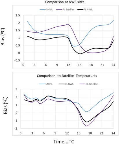
However, NWS observation sites are relatively coarse (60–80 km versus grid resolutions 4–12 km) and may not capture actual land use gradients. Diak (1990), Anderson et al. (1997), McNider et al. (1994), and McNider et al. (2005) showed that satellite observations have the potential to recover unobserved land use parameters that standard surface observations cannot resolve. McNider et al. (2018) incorporated satellite observations into the Pleim-Xiu land surface model. A series of model experiments on a 12-km resolution national domain were carried out, employing satellite assimilation techniques for a month-long period (September 2013). Details on the satellite data sets and sequential inclusion of different satellite assimilation components are provided in McNider et al. (2018). The satellite data included a satellite insolation product (McNider, Norris, and Song 1995), a satellite vegetative greenness (a composite property of leaf area, chlorophyll and canopy structure) product (Case et al. 2014) similar to Ran et al. (2016), and satellite-derived skin temperature. The technique employed a morning satellite skin temperature for moisture adjustment similar to the Pleim-Xiu NWS adjustment, and nighttime satellite skin temperature for surface heat capacity similar to the Pleim and Gilliam (2009) deep soil temperature adjustment. Here, we provide in Figure 13 the impact of the satellite assimilation on temperatures in the Great Lakes Region compared to the NWS assimilation.

Figure 13 top shows the result of the satellite assimilation as compared to NWS observations. The results show that the improvement in daytime performance is very close to that of the Pleim-Xiu-Gilliam soil moisture NWS-based adjustment scheme. However, the satellite heat capacity adjustment does not correct nighttime temperatures as much as the Pleim-Gilliam deep temperature scheme.

Water surface specification

While the above discussion has focused on land surface modeling, lower boundary conditions especially over water can also be important in regional air quality simulations. Also, reduced deposition velocities especially for ozone and precursors over water can be important relative to deposition over land (Qin et al. 2019).

In air quality work, almost all modeling has used fixed boundary conditions over water for temperature based on external analyses with temperature-dependent saturation conditions used for humidity. NOAA or NASA generally provides these temperature analyses. Appel (2014) initially used the temperature 12 km analysis in the NAM-12 reanalysis product but switched to a high-resolution temperature product (https://www.ghrsst.org/) from the Advanced Very-High Resolution Radiometer (AVHRR) satellite which provides twice daily composite SST measurements at 1-km grid spacing. Appel et al. found that it greatly improved water temperatures over the smaller bays and inlets in the complex Chesapeake Bay area and improved model performance. See Figure 14 taken from Appel (2014).

Figure 14. Left, skin temperature (K) field using the NAM 12-km data. Right – skin temperature (K) field using the GHR-SST 1-km data. From Appel (2014).

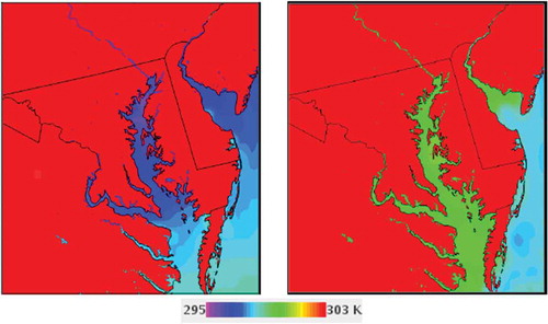
Fast and Heilman (2003) carried out a study of the impact of water temperatures in the development of the boundary layer and circulations over the Great Lakes and made comparison between model and buoy temperatures. More recently, McNider et al. (2018) examined the differences in water surface temperatures and their impact over the Great Lakes (Figure 15). For a 2009 case study, two different water temperature analyses were evaluated. WRF model simulations employed the standard NAM-12 SST product, which were based on the NOAA temperature analysis product (based on Great Lakes Environmental Research Laboratory (GLERL) SST data set – https://www.glerl.noaa.gov/res/glcfs). A second SST product based on MODIS satellite data (Kilpatrick et al. 2015) was also used in WRF. First, a direct comparison was made of the two temperature products with buoy data. For two Lake Michigan buoys, the comparison showed that the average buoy water temperatures were slightly warmer than the GLERL temperatures but only lees than about 0.5 C. The MODIS temperatures were on average colder by about 2–3C. What was clear in the comparison is that the observed data had about a 1–2 degree diurnal cycle in temperature that was not included in the analyses. As discussed by McNider et al. (2018), this may present problems in that the lowest layer air temperature has a physically radiative cooling diurnal component, which may then be inconsistent with the imposed water temperatures in the analyses.

Figure 15. Time series of SST or water temperature for two Lake Michigan buoys compared to GLERL and MODIS lake temperatures for the simulation period of 01 July to 04 September 2009. Buoy water temperature measurement is at approximately 0.6 m. The MODIS is a skin temperature and GLERL a blended temperature. From McNider et al. (2018).

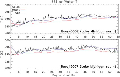
Comparisons were also made of the WRF air temperature and wind to buoy observations over the Great Lakes using the two water temperature data sets. The comparative analyses showed that the modeled air temperatures using the GLERL water temperatures were about 2C cooler than buoy air temperatures and air temperature using MODIS were another 2C cooler. This was larger than changes in air temperature due to different PBL schemes.

Land use changes, urbanization and aerosols impacting the model surface

With growing populations and migration into cities, especially in the developing world, land use change is a growing consideration for land surface modeling. Civerolo et al. (2000) cautioned against using historical land use for future year air quality predictions. Additionally, aerosol loading can also impact land surface energetics (Nair et al. 2011; Petäjä et al. 2016). Fortunately, satellite products for land use classification and albedo have become more routinely available (Ran et al. 2016). In addition to land surface energetic reductions in vegetative cover can also impact the stomatal uptake of ozone (Wu et al. 2012).

Aerosols and climate have been a major concern because of the cooling effect of aerosols. Xing et al. (2015) demonstrated that coupled meteorological and air quality could capture trends in aerosol optical depth that impact surface radiation over long time scales and shorter time scales (Hogrefe et al. 2015). Petäjä et al. (2016) showed that aerosols can reduce incoming radiation inhibiting the growth of the PBL, which in turn increases boundary layer pollutant concentrations. Jacobson (1998) and Nair et al. (2011) showed that aerosols can interact with the highly non-linear nighttime stable boundary layer to increase mixing and the downward flux of heat, momentum and pollutants above the SBL. These aerosol effects can be especially important in the developing world.

In addition to energetic impacts at the surface, aerosols can have an impact on photolysis rates. Jacobson (1998) showed that aerosols can reduce boundary layer photolysis rates and showed that impacts of aerosols in Los Angeles simulations decreased ozone levels basin wide by 5–8%. The photolysis impacts alone would likely be greater since aerosols can decrease vertical mixing through the reduction in surface energy tending to increase concentrations. There are also chemical pathways that are altered by aerosols (Jacobson 1998).

Model performance in predicting clouds

As discussed in the introduction, clouds can be a critical parameter in air quality modeling. First, clouds modulate the incoming solar radiation that controls temperature and turbulence at the surface. Second, clouds directly impact photochemical rates (Madronich 2016). Third, clouds impact Biogenic Volatile Organic Carbon (BVOC) emissions (Zhang et al. 2018). Fourth, clouds impact venting out of the boundary layer into the free troposphere (Angevine, Jiang, and Mauritsen 2010). The correct development of clouds in space and time within numerical meteorological models is essential for producing an accurate representation of the physical atmosphere for input into air quality models.

The representation of clouds in models has always been problematic, because clouds depend on parametrizations of cloud liquid water and ice processes. Second, even small mesoscale circulations can change the environmental support (humidity, temperature, vertical motions) for clouds in space and time. Third, historical operational cloud observations are not direct in terms of fundamental model parameters such as cloud liquid water or ice. Recent cloud observational networks, especially in Europe (Hogan, O’Connor, and Illingworth 2009) have begun to provide more routine observations, though sparse in space. More recently, surface solar radiation measurements that integrate cloud and ice radiative effects have been used for model evaluation (Yang et al. 2006). While surface solar radiation is also parameterized, it directly reflects the impact of clouds on incoming solar energy. Cloud modeling has improved over the last 10 years in paired in space and time statistics. However, significant scatter between model and observed data remain when using solar radiation data as a metric (Pour‐Biazar et al. 2007; White et al. 2018; Yang and Friedl 2003).

While surface measurements of solar radiation have increased in recent years, they are still coarse relative to standard measurements such as temperature and wind. There are only about 230 pyranometer sites under the two major U.S. networks (SURFRAD and SCAN networks) compared to approximately 6000 surface meteorological observation sites. Since geostationary satellites have the capability to view clouds and their temporal development, there have been methods to retrieve solar insolation from satellite visible reflectance data (Diak and Gautier 1983; Gautier, Diak, and Masse 1980) to provide improved spatial information. Though satellites can visually capture clouds through visible instrumentation channels, this methodology is simply a measure of cloud reflectance. Though important, this is only one aspect of clouds. In order to convert to surface radiance (watts/m²), auxiliary information is needed, e.g. surface albedo, instrumentation calibration, clear sky absorption, etc. Thus, satellite insolation is still an estimate. The advent of more surface insolation data has allowed a more stringent evaluation of these satellite retrievals. Figure 16 shows a recent evaluation of several satellite insolation products carried out during the Discover-AQ 2013 program for September 1–30, 2103. The scatter in these comparisons reflects uncertainty in satellite retrieval components, but also represent to some extent the difference between the point pyranometer measurements and the satellite resolution of approximately 4 km for GOES insolation products. Thus, some of the scatter is because the satellite retrieval represents the spatial average insolation retrieved from an instantaneous image and the pyranometer measurement represents some temporal average over a point that may or may not be exposed to the clouds seen in the satellite image. In total, some of the scatter represent the irreducible uncertainty in comparing point measurement to the area-averaged quantity.

Figure 16. Satellite-derived insolation products (left axis) versus pyranometer measurements (bottom axis). Units are Wm⁻² (left) NOAA GSIP satellite insolation product versus pyranometer observation. (middle) NASA-UAH Sport satellite insolation product versus pyranometer observation. (right) WRF insolation. Black line indicates 1:1 ratio. At the top of each plot are the regression equations and the Root Mean Square Errors (RMSE) designated by the “sigma” symbol. The sigma values are in units of W m⁻². Note larger scatter (σ = 144.2 W m⁻²compared to 102.6 W m⁻² for GSIP satellite product) in WRF insolation which represents error in time and place of model clouds. Developed under NASA Applied Science Air Quality Team (AQAST) activities.

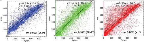
Also, shown in the right panel is a comparison of WRF insolation to pyranometer observations. It shows that the scatter between model and observations is approximately 50% greater than between satellite insolation and observations. The greater spread between the model and observations represent errors in the placement and timing of model clouds. In air quality modeling, the representation of clouds in the meteorological model (or in some cases re-diagnosed clouds in the chemistry model) controls energy inputs to the surface and photolysis rates. Thus, the satellite products provide a better measure of clouds paired in space and time than do models.

Several investigators have attempted to assimilate the satellite observations directly into meteorological models (Lipton and Modica 1999; Pincus et al. 2011; Yucel et al. 2003). However, this continues to be a challenge due to the relatively primitive cloud parameterizations (see Bauer et al. 2011). McNider et al. (1998a) instead used satellite insolation directly in place of meteorological model insolation and showed improvement in model performance. Solar insolation values were improved by 150% compared to pyranometer measurements and temperatures were improved by 3–5 C in places where clouds were misplaced in the model. Pour‐Biazar et al. (2007) replaced model cloud reflectance with satellite reflectance to calculate chemical photolysis rates. Figure 17 shows the difference in ozone concentration between the satellite photolysis rates and model photolysis rates. It shows significant differences between the two and that the satellite photolysis improves model performance at points where the differences exist. Tang et al. (2015) used a similar approach within the WRF-CAMx modeling system and demonstrated improved ozone simulation over east Texas. Ryu et al. (2017, 2018) also corrected the radiative impact of clouds in WRF-Chem by replacing model photolysis and photosynthetically active radiation (PAR) with the estimates based on satellite observation and attempted to quantify model errors in surface ozone simulations due to model cloud errors. Ryu et al. (2018) reported that about 40% of the bias (1–5 ppb) for maximum daily 8-h average ozone under cloudy conditions (for their summer case study) is due to model cloud errors. These model errors caused hourly biases of up to 60 ppb.

Figure 17. Top figure shows the differences in ozone between two CMAQ runs with and without use of satellite-derived photolysis fields (units are ppb of ozone). Note the maximum differences exceed 50 ppb. Bottom figure shows the time series of ozone predictions from the model vs. observations at an EPA monitoring site in South Mississippi. The monitor location is approximately denoted by the apex of the black lines Adapted from two figures in Pour‐Biazar et al. (2007).

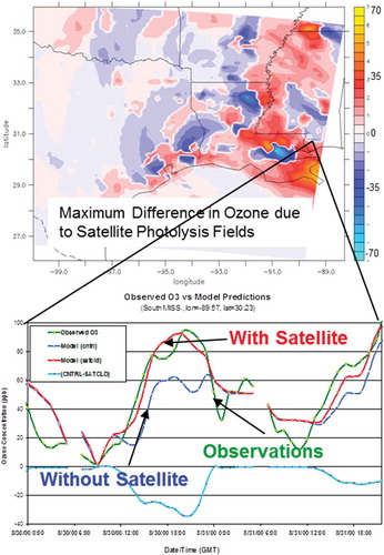
As acknowledged by previous studies (Pour‐Biazar et al. 2007; Tang et al. 2015), while direct insertion of satellite insolation or satellite reflectance can improve the location of clouds and photochemical model performance, it introduces consistency problems in that other model cloud attributes (e.g. cloud water) no longer exist at the same time and location as the satellite observation. Thus, moist chemistry and cloud mixing are misaligned. It would be better to have clouds in the meteorological model agree better with satellite clouds.

There have been past attempts at using satellite data to improve model cloud performance. These have largely followed inserting satellite-derived liquid water into the model domain. Lipton and Modica (1999) used GOES-7 data to adjust the model relative humidity field in stratiform cloud areas and found a general improvement in the model simulation (bias was reduced from −0.9C to 0.4C and standard error was reduced from 1.6C to 1.4C), but only for a very short time. In a fundamental physical sense, clouds form where atmospheric lifting is occurring and cloud-free areas are largely where subsidence is occurring. If the model does not have clouds at a location that the satellite has clouds, then you are inserting water where there is likely subsidence. Thus, any water inserted will likely evaporate, producing even further subsidence. This has been the problem with direct cloud water insertion or adjusting relative humidity to saturation. Clouds formed as the result of water insertion will not last and can make the model worse. Yucel et al. (2003) discovered that adjustment of the model dynamics and thermodynamics was necessary to utilize fully the observed cloud information within MM5. White et al. (2018) developed a mass-consistent variational technique (O’Brien 1970) in which lifting and subsidence are diagnosed from satellite cloud observation. The technique is based on providing dynamical lifting or subsidence to support cloud development or cloud clearing. Where the satellite data indicate clouds exist but are not in the model, the technique provides lifting until clouds form. Where the satellite shows clear sky but the model has clouds, the technique provides subsidence until clouds disappear.

White et al. (2018) used a contingency table to define an evaluation metric called the Cloud Agreement Index, which is used below. The AI is defined as

$\mathrm{A}\mathrm{I}=\left(\mathrm{A}+\mathrm{D}\right)/\left(\mathrm{A}+\mathrm{B}+\mathrm{C}+\mathrm{D}\right)$

where A and D are categories for the number of times the model and GOES agree on clouds and B and C are the number of times they disagree. Table 1 defines the categories.

Table 1. Contingency table used to derive the Index of Agreement. A, B, C and D are the number of events falling in that category. For example A is the number of times both WRF and GOES have the same grid to be cloudy. C is the number of times WRF says it is cloudy but GOES shows clear. The color corresponds to the colors used in the spatial depictions of agreement.

The simulations were performed on 36-, 12- and 4-km grid size domains covering the Contiguous United States, South-Southeastern U.S. and Eastern Texas, respectively. The technique was tested over the month of August 2006. Figure 18 shows the spatial depiction of the Agreement Index. The results indicated that the assimilation technique significantly improved the agreement between the model-predicted and GOES-derived cloud fields. The daily average percentage increase in the cloud AI was determined to be 14.02%, 11.29% and 4.96% for the 36-, 12- and 4-km domains, respectively. This was accomplished without degrading and in some cases improving the model performance with respect to surface wind speed, temperature and mixing ratio, which are important parameters for air quality applications. The cloud assimilation decreased the bias between pyranometer observations and the model at every location.

Figure 18. The spatial agreement between the model and GOES cloud fields for (A) CNTRL and (B) Cloud Assimilation on August 12, 2006 at 17 UTC for the 36-km simulation. Green represents locations where the model and GOES were clear, red is locations where the model is cloudy and GOES is clear, orange is areas where the model is clear when GOES is cloudy, and gray is locations where both the model and GOES were cloudy. The AI is the percentage of grids within the domain that are in agreement with GOES. From White et al. (2018).

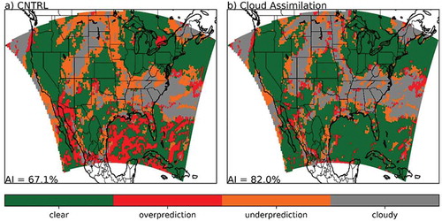
The GOES cloud assimilation improves surface solar radiation, which is important for energy into land surface. In comparing model insolation with and without satellite data, the case using GOES observation reduced the bias in insolation measured at pyranometers around the country. This also would improve the specification of photolysis rates and solar forcing of biogenic emissions.

Biogenic emissions are dependent on photosynthetically active radiation (PAR) and temperature. Clouds suppress PAR and temperature so their paired in space and time behavior are critical for biogenic emission rates. Pinker and Laszlo (1992) recognized the importance of PAR to biophysical systems and developed products to serve the air quality and agricultural communities. Standard calculations in models such as WRF-CMAQ use a fixed conversion factor of 0.5 to recover PAR from the WRF insolation field. PAR generally relates to solar insolation, but the narrower wavelength bands for PAR are more affected by solar angle and atmospheric path length. Pour-Biazar et al. (2015) developed a correction factor to convert solar insolation to PAR based on solar zenith angle and cloud optical depth.

Zhang et al. (2018) carried out experiments to examine the impact of different PAR products on biogenic emissions within the MEGAN biogenic emission model (for a study in Texas). Figure 19 shows the comparisons of recovered PAR from three different techniques with observed PAR. The three cases are (1) the WRF default case where PAR is recovered using a constant correction factor (0.5) to recover PAR from model-predicted insolation fields; (2) the assimilation of GOES clouds into WRF described above by White et al. (2018) and (3) the direct use of GOES insolation using the Pour-Biazar et al. (2015) correction factor. It shows that the GOES cloud assimilation case and the direct use of GOES retrieved PAR produce a better agreement with observations. At some locations, correlations were improved by 0.1 and mean bias by 25%. However, in using the three PAR products in MEGAN there was less clear agreement on which produced the better air quality impacts. This may be due to the fact that while the use of satellite-derived PAR resulted in 20% reduction in isoprene emission rate (and 5% reduction in terpene emission rate), the reduction was not large enough to offset model overestimation due to other compensating errors in MEGAN (and also lack of direct VOC measurements).

Figure 19. Correlation and mean normalized bias (NMB) at TCEQ sites for photosynthetically active radiation (PAR). Observations of PAR at these sites are compared with model estimates simulated by the (left) WRF base case (middle) WRF with assimilated clouds, and direct estimates from (right) UAH GOES retrievals. From Zhang et al. (2018).

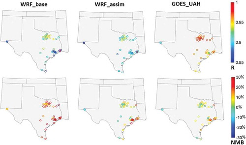
Ryu et al. (2018) indicated that in their study photolysis rate had a larger impact on surface ozone than BVOC emissions (80% on average). They concluded that the contribution of BVOC emissions to O₃ can be important in areas with high NOx source and low VOC (VOC-limited regimes) that even small increases in VOC has a great impact on ozone production (e.g., cities of the southeastern U.S.)

Further thoughts

Since acid rain and ozone concerns in the late 1970s brought gridded meteorological modeling as a tool to the air quality community, there has been a consistent improvement in models and techniques. The above review attempts to capture these improvements and continual challenges for the future. However, it cannot cover all the actions that have improved models or the advances in observations and model evaluation techniques.

There has been a considerable improvement in the quality and tools for incorporating both traditional observations and new tools such as satellite data and profiler data for retrospective studies. However, as community models such as WRF have become a mainstay, there are now literally hundreds of options available for selection. It would seem that there is a community need to evaluate and recommend sets of options that provide important performance measures.

Acknowledgments

The authors wish to acknowledge the support of various entities over many years for their support of investigations into the role of the physical atmosphere in air quality concerns. These include U.S. EPA, U.S. DOE, NASA, EPRI, NOAA, the Bureau of Ocean Energy Management (formerly, Minerals Management Service), the State of Texas and the State of Alabama. The results in this review do not necessarily reflect the views of the funding agencies. The authors also wish to thank members of their research teams over the years that have carried out these studies, especially Kevin Doty, Yu Ling Wu, Aaron Song, Scott Makaro and Andrew White. We also wish to thank the three reviewers of this manuscript whose comments greatly improved the quality and content of the manuscript.

Disclosure statement

No potential conflict of interest was reported by the authors.

Additional information

Notes on contributors

Richard T. McNider

Dr. Richard T. McNider is distinguished Professor of science, emeritus, at the University of Alabama in Huntsville (UAH), Huntsville, Alabama.

Arastoo Pour-Biazar

Dr. Arastoo Pour-Biazar is a research scientist at the Earth System Science Center, University of Alabama in Huntsville, Huntsville, Alabama.

References

- Altshuiler, A. P. 1978. Association of oxidant episodes with warm stagnating anticyclones. J. Air Pollut. Control Assoc. 28 (2):152–55. doi:10.1080/00022470.1978.10470585.
- Anav, A., A. De Marco, P. Friedlingstein, F. Savi, P. Sicard, S. Sitch, M. Vitale, and E. Paoletti. 2019. Growing season extension affects ozone uptake by European forests. Sci. Total Environ. 669:1043–52. doi:10.1016/j.scitotenv.2019.03.020.
- Anav, A., C. Proietti, L. Menut, S. Carnicelli, A. D. Marco, and E. Paoletti. 2018. Sensitivity of stomatal conductance to soil moisture: Implications for tropospheric ozone. Atmos. Chem. Phys. 18 (8):5747–63. doi:10.5194/acp-18-5747-2018.
- Anderson, M. C., J. M. Norman, G. R. Diak, W. P. Kustas, and J. R. Mecikalski. 1997. A two-source time-integrated model for estimating surface fluxes using thermal infrared remote sensing. Remote Sens. Environ. 60:195–216. doi:10.1016/S0034-4257(96)00215-5.
- Angevine, W. M., C. J. Senff, A. B. White, E. J. Williams, J. Koermer, S. T. Miller, R. Talbot, P. E. Johnston, S. A. McKeen, and T. Downs. 2004. Coastal boundary layer influence on pollutant transport in New England. J. Appl. Meteorol. 43 (10):1425–37. doi:10.1175/JAM2148.1.
- Angevine, W. M., H. Jiang, and T. Mauritsen. 2010. Performance of an eddy diffusivity–Mass flux scheme for shallow cumulus boundary layers. Mon. Weather Rev. 138 (7):2895–912. doi:10.1175/2010MWR3142.1.
- Angevine, W. M., J. Brioude, S. McKeen, and J. S. Holloway. 2014. Uncertainty in Lagrangian pollutant transport simulations due to meteorological uncertainty from a mesoscale WRF ensemble. Geosci. Model Dev. 7:2817–29. doi:10.5194/gmd-7-2817-2014.
- Anthes, R. A., and T. T. Warner. 1978. Development of hydrodynamic models suitable for air pollution and other mesometerological studies. Mon. Weather Rev. 106 (8):1045–78. doi:10.1175/1520-0493(1978)106<1045:DOHMSF>2.0.CO;2.
- Appel, K. W., A. B. Gilliland, G. Sarwar, and R. C. Gilliam. 2007. Evaluation of the community multiscale air quality (CMAQ) model version 4.5: Sensitivities impacting model performance: Part I—Ozone. Atmos. Environ. 41 (40):9603–15. doi:10.1016/j.atmosenv.2007.08.044.
- Appel, W.; Coauthors. 2014. Improvements to the WRF-CMAQ modeling system for fine-scale air quality simulations. EM Mag. 14:16–21.
- Astitha, M., H. Luo, S. T. Rao, C. Hogrefe, R. Mathur, and N. Kumar. 2017. Dynamic evaluation of two decades of WRF-CMAQ ozone simulations over the contiguous United States. Atmos. Environ. 164:102–16. doi:10.1016/j.atmosenv.2017.05.020.
- Baker, K. R., H. Simon, and J. T. Kelly. 2011. Challenges to modeling “cold pool” meteorology associated with high pollution episodes. Environ. Sci. Technol. 2011 (45):7118–19. doi:10.1021/es202705v.
- Banks, R. F., J. Tiana-Alsina, J. M. Baldasano, F. Rocadenbosch, A. Papayannis, S. Solomos, and C. G. Tzanis. 2016. Sensitivity of boundary-layer variables to PBL schemes in the WRF model based on surface meteorological observations, lidar, and radiosondes during the HygrA-CD campaign. Atmos. Res. 176:185–201. doi:10.1016/j.atmosres.2016.02.024.
- Banta, R. M., C. J. Senff, J. Nielsen-Gammon, L. S. Darby, T. B. Ryerson, R. J. Alvarez, S. P. Sandberg, E. J. Williams, and M. Trainer. 2005. A bad air day in Houston. Bull. Am. Meteorol. Soc. 86 (5):657–70. doi:10.1175/BAMS-86-5-657.
- Barna, M., and B. Lamb. 2000. Improving ozone modeling in regions of complex terrain using observational nudging in a prognostic meteorological model. Atmos. Environ. 34 (28):4889–906. doi:10.1016/S1352-2310(00)00231-4.
- Bauer, P., G. Ohring, C. Kummerow, and T. Auligne. 2011. Assimilating satellite observations of clouds and precipitation into NWP models. Bull. Am. Meteorol. Soc. 92 (6):ES25–ES28. doi:10.1175/2011BAMS3182.1.
- Beljaars, A. C. M. 1995. The impact of some aspects of the boundary layer scheme in the ECMWF model. In Proceedings of Seminar on parametrization of sub-grid scale physical processes, 125–62. 5–9 September 1994, ECMWF, Reading, UK.
- Beljaars, A. C. M., and A. A. M. Holtslag. 1991. Flux parameterization over land surfaces for atmospheric models. J. Appl. Meteorol. 30 (3):327–41. doi:10.1175/1520-0450(1991)030<0327:FPOLSF>2.0.CO;2.
- Berman, S., J. Y. Ku, J. Zhang, and S. T. Rao. 1997. Uncertainties in estimating the mixing depth-comparing three mixing-depth models with profiler measurements. Atmos. Environ. 31 (18):3023–3039. doi:10.1016/S1352-2310(97)00118-0.
- Biswas, J., and S. T. Rao. 2001. Uncertainties in episodic ozone modeling stemming from uncertainties in meteorological fields. J. Appl. Meteorol. 40:117–36. doi:10.1175/1520-0450(2001)040<0117:UIEOMS>2.0.CO;2.
- Blackadar, A. K. 1957. Boundary layer wind maxima and their significance for the growth of nocturnal inversions. Bull. Am. Meteorol. Soc. 283–90. doi:10.1175/1520-0477-38.5.283.
- Blackadar, A. K. 1979. High resolution models of the planetary boundary layer. In Advances in environmental science and engineering, 50–85. Gordon and Breach.
- Bonner, W. D., and J. Paegle. 1970. Diurnal variations in boundary layer winds over the south-central United States in summer. Mon. Weather Rev. 98 (10):735–44. doi:10.1175/1520-0493(1970)098<0735:DVIBLW>2.3.CO;2.
- Bornstein, R. D., and W. T. Thompson. 1981. Effects of frictionally retarded sea breeze and synoptic frontal passages on sulfur dioxide concentrations in New York City. J. Appl. Meteorol. 20 (8):843–58. doi:10.1175/1520-0450(1981)020<0843:EOFRSB>2.0.CO;2.
- Bosveld, F. C., P. Baas, G. J. Steeneveld, A. A. Holtslag, W. M. Angevine, E. Bazile, E. I. de Bruijn, D. Deacu, J. M. Edwards, M. Ek, et al. 2014. The third GABLS intercomparison case for evaluation studies of boundary-layer models. Part B: Results and process understanding. Boundary Layer Meteorol. 152 (2):157–87. doi:10.1007/s10546-014-9919-1.
- Bougeault, P., and P. Lacarrere. 1989. Parameterization of orography-induced turbulence in a mesobeta–Scale model. Mon. Weather Rev. doi:10.1175/1520-0493(1989)117<1872:POOITI>2.0.CO;2.
- Businger, J. A. 1973. Turbulent transfer in the atmospheric surface layer. Amer. Meteorol. Soc. 67–100.
- Byun, D., and K. L. Schere. 2006. Review of the governing equations, computational algorithms, and other components of the model-3 community multiscale air quality (CMAQ) modeling system. Appl. Mech. Rev. 59 (2):51–77. doi:10.1115/1.2128636.
- Byun, D. W., J. Young, J. Pleim, M. T. Odman, and K. Alapaty. 1999. Numerical transport algorithms for the community multiscale air quality (CMAQ) chemical transport model in generalized coordinates. Science Algorithms of the EPA Models-3 Community Multiscale Air Quality (CMAQ) Modeling System.
- Camalier, L., W. Cox, and P. Dolwick. 2007. The effects of meteorology on ozone in urban areas and their use in assessing ozone trends. Atmos. Environ. 41 (33):7127–37. doi:10.1016/j.atmosenv.2007.04.061.
- Canty, T. P., L. Hembeck, T. P. Vinciguerra, D. L. Goldberg, S. F. Carpenter, D. J. Allen, C. P. Loughner, R. J. Salawitch, and R. R. Dickerson. 2015. Ozone and NOx chemistry in the eastern US: Evaluation of CMAQ/CB05 with satellite (OMI) data. Atmos. Chem. Phys. 15 (19):10965. doi:10.5194/acp-15-10965-2015.
- Cardelino, C. A., and W. L. Chameides. 1995. An observation-based model for analyzing ozone precursor relationships in the urban atmosphere. J. Air Waste Manage. Assoc. 45 (3):161–80. doi:10.1080/10473289.1995.10467356.
- Carlson, T. N. 1986. Regional‐scale estimates of surface moisture availability and thermal inertia using remote thermal measurements. Remote Sens. Rev. 1 (2):197–247. doi:10.1080/02757258609532069.
- Case, J. L., F. J. LaFontaine, J. R. Bell, G. J. Jedlovec, S. V. Kumar, and C. D. Peters-Lidard. 2014. A real-time MODIS vegetation product for land surface and numerical weather prediction models. IEEE Trans. Geosci. Remote Sens. 52 (3):1772–86. doi:10.1109/TGRS.2013.2255059.
- Castellanos, P., L. T. Marufu, B. G. Doddridge, B. F. Taubman, J. J. Schwab, J. C. Hains, S. H. Ehrman, and R. R. Dickerson. 2011. Ozone, oxides of nitrogen, and carbon monoxide during pollution events over the eastern United States: An evaluation of emissions and vertical mixing. J. Geophys. Res. 116:D16307. doi:10.1029/2010JD014540.
- Chen, F., and J. Dudhia. 2001. Coupling an advanced land surface-hydrology model with the Penn State-NCAR MM5 modeling system. Part I: Model implementation and sensitivity. Mon. Weather Rev. 129:569–85. doi:10.1175/1520-0493(2001)129<0569:CAALSH>2.0.CO;2.
- Chen, Y., J. An, Y. Sun, X. Wang, Y. Qu, J. Zhang, Z. Wang, and J. Duan. 2018. Nocturnal low-level winds and their impacts on particulate matter over the Beijing area. Adv. Atmos. Sci. 35:1455. doi:10.1007/s00376-018-8022-9.
- Cheng, W. Y. Y., and W. J. Steenburgh. 2005. Evaluation of surface sensible weather forecast by the WRF and the Eta Models over the western United States. Weather Forecasting 20:812–21. doi:10.1175/WAF885.1.
- Ching, J. K. S. 2013. A perspective on urban canopy layer modeling for weather, climate and air quality applications. Urban Clim. 3:13–39. doi:10.1016/j.uclim.2013.02.001.
- Ching, J. K. S., and A. J. Alkezweeny. 1986. Tracer study of vertical exchange by cumulus clouds. J. Clim. Appl. Meteorol. 25 (11):1702–11. doi:10.1175/1520-0450(1986)025<1702:TSOVEB>2.0.CO;2.
- Cimorelli, A. J., S. G. Perry, A. Venkatram, J. C. Weil, R. J. Paine, R. B. Wilson, R. F. Lee, W. D. Peters, and R. W. Brode. 2005. AERMOD: A dispersion model for industrial source applications. Part I: General model formulation and boundary layer characterization. J. Appl. Meteorol. 44 (5):682–93. doi:10.1175/JAM2227.1.
- Civerolo, K. L., G. Sistla, S. T. Rao, and D. J. Nowak. 2000. The effects of land use in meteorological modeling: Implications for assessment of future air quality scenarios. Atmos. Environ. 34 (10):1615–21. doi:10.1016/S1352-2310(99)00393-3.
- Cleary, P. A., N. Fuhrman, L. Schulz, J. Schafer, J. Fillingham, H. Bootsma, J. McQueen, Y. Tang, T. Langel, S. McKeen, et al. 2015. Ozone distributions over southern Lake Michigan: Comparisons between ferry-based observations, shoreline-based DOAS observations and model forecasts. Atmos. Chem. Phys. 15 (9):5109–22. doi:10.5194/acp-15-5109-2015.
- Cohen, A. E., S. M. Cavallo, M. C. Coniglio, and H. E. Brooks. 2015. A review of planetary boundary layer parameterization schemes and their sensitivity in simulating southeastern US cold season severe weather environments. Weather Forecasting 30 (3):591–612. doi:10.1175/WAF-D-14-00105.1.
- Cooper, O. R., M. Trainer, A. M. Thompson, S. J. Oltmans, D. W. Tarasick, J. C. Witte, A. Stohl, S. Eckhardt, J. Lelieveld, M. J. Newchurch, et al. 2007. Evidence for a recurring eastern North America upper tropospheric ozone maximum during summer. J. Geophys. Res. Atmos. 112:D23. doi:10.1029/2007JD008710.
- Cox, W. M., and S. H. Chu. 1996. Assessment of interannual ozone variation in urban areas from a climatological perspective. Atmos. Environ. 30 (14):2615–25. doi:10.1016/1352-2310(95)00346-0.
- Dai, A., K. E. Trenberth, and T. R. Karl. 1999. Effects of clouds, soil moisture, precipitation, and water vapor on diurnal temperature range. J Clim 12 (8):2451–73. doi:10.1175/1520-0442(1999)012<2451:EOCSMP>2.0.CO;2.
- Dennis, R., T. Fox, M. Fuentes, A. Gilliland, S. Hanna, C. Hogrefe, J. Irwin, S. T. Rao, R. Scheffe, K. Schere, et al. 2010. A framework for evaluating regional-scale numerical photochemical modeling systems. Environ. Fluid Mech. 10 (4):471–89. doi:10.1007/s10652-009-9163-2.
- Diak, G. R. 1990. Evaluation of heat flux, moisture flux and aerodynamic roughness at the land surface from knowledge of the PBL height and satellite-derived skin temperatures. J. Agric. For. Meteorol. 52:181–98. doi:10.1016/0168-1923(90)90105-F.
- Diak, G. R., and C. Gautier. 1983. Improvements to a simple physical model for estimating insolation from GOES data. J. Clim. Appl. Meteorol. 22 (3):505–08. doi:10.1175/1520-0450(1983)022<0505:ITASPM>2.0.CO;2.
- Dueñas, C., M. C. Fernández, S. Cañete, J. Carretero, and E. Liger. 2002. Assessment of ozone variations and meteorological effects in an urban area in the Mediterranean Coast. Sci. Total Environ. 299 (1–3):97–113.
- Dye, T. S., P. T. Roberts, and M. E. Korc. 1995. Observations of transport processes for ozone and ozone precursors during the 1991 Lake Michigan Ozone Study. J. Appl. Meteorol. 34 (8):1877– 89. doi:10.1175/1520-0450(1995)034%3C1877:OOTPFO%3E2.0.CO;2.
- Edwards, J. M., R. J. Beare, and A. J. Lapworth. 2006. Simulation of the observed evening transition and nocturnal boundary layers: Single‐column modelling. Q. J. R. Meteorolog. Soc. 132 (614):61–80. doi:10.1256/qj.05.63.
- Egan, B. A., and J. R. Mahoney. 1972. Numerical modeling of advection and diffusion of urban area source pollutants. J. Appl. Meteorol. 11 (2):312–22. doi:10.1175/1520-0450(1972)011<0312:NMOAAD>2.0.CO;2.
- Ek, M. B., K. E. Mitchell, Y. Lin, E. Rogers, P. Grunmann, V. Koren, G. Gayno, and J. D. Tarpley. 2003. Implementation of Noah land surface model advances in the national centers for environmental prediction operational mesoscale Eta model. J. Geophys. Res. Atmos. 108:D22. doi:10.1029/2002JD003296.
- Eliassen, A. 1980. A review of long-range transport modeling. J. Appl. Meteorol. 19 (3):231–40. doi:10.1175/1520-0450(1980)019<0231:AROLRT>2.0.CO;2.
- England, D. E., and R. T. McNider. 1995. Stability functions based upon shear functions. Boundary Layer Meteorol. 74:113–30. doi:10.1007/BF00715713.
- ENVIRON. 2013. User’s guide to the comprehensive air quality model with extensions, version 6. http://www.camx.com/Files/CAMxUsersGuide_v6-00.pdf.
- EPA. 2018. https://www.epa.gov/scram/state-implementation-plan-sip-attainment-demonstration-guidance#8ozone.
- Esau, I. N., and Ø. Byrkjedal. 2007. Application of a large-eddy simulation database to optimisation of first-order closures for neutral and stably stratified boundary layers. Boundary Layer Meteorol. 125 (2):207–25. doi:10.1007/s10546-007-9213-6.
- Fast, J. D. 1995. Mesoscale modeling and four-dimensional data assimilation in areas of highly complex terrain. J. Appl. Meteorol. 34 (12):2762–82. doi:10.1175/1520-0450(1995)034<2762:MMAFDD>2.0.CO;2.
- Fast, J. D., and C. M. Berkowitz. 1996. A modeling study of boundary layer processes associated with ozone layers observed during the 1993 North Atlantic regional experiment. J. Geophys. Res. Atmos. 101 (D22):28683–99. doi:10.1029/96JD02958.
- Fast, J. D., and W. E. Heilman. 2003. The effect of lake temperatures and emissions on ozone exposure in the western Great Lakes region. J. Appl. Meteorol. 42 (9):1197–217. doi:10.1175/1520-0450(2003)042<1197:TEOLTA>2.0.CO;2.
- Foley, K. M., C. Hogrefe, G. Pouliot, N. Possiel, S. J. Roselle, H. Simon, and B. Timin. 2015a. Dynamic evaluation of CMAQ part I: Separating the effects of changing emissions and changing meteorology on ozone levels between 2002 and 2005 in the eastern US. Atmos. Environ. 103:247–55. doi:10.1016/j.atmosenv.2014.12.038.
- Foley, K. M., P. Dolwick, C. Hogrefe, H. Simon, B. Timin, and N. Possiel. 2015b. Dynamic evaluation of CMAQ part II: Evaluation of relative response factor metrics for ozone attainment demonstrations. Atmos. Environ. 103:188–95. doi:10.1016/j.atmosenv.2014.12.039.
- Foley, T., E. A. Betterton, P. R. Jacko, and J. Hillery. 2011. Lake Michigan air quality: The 1994–2003 LADCO Aircraft Project (LAP). Atmos. Environ. 45 (18):3192–202. doi:10.1016/j.atmosenv.2011.02.033.
- Fovell, R. 2013. WRF performance issues in the San Joaquin Valley and Southern California. In Traversing New Terrain in meteorological modeling for air quality and dispersion. Davis, CA: U.California, September 9–11.
- Gan, C. M., J. Pleim, R. Mathur, C. Hogrefe, C. N. Long, J. Xing, D. Wong, R. Gilliam, and C. Wei. 2015. Assessment of long-term WRF–CMAQ simulations for understanding direct aerosol effects on radiation” brightening” in the United States. Atmos. Chem. Phys. 15 (21):12193–209. doi:10.5194/acp-15-12193-2015.
- García‐Díez, M., J. Fernández, L. Fita, and C. Yagüe. 2013. Seasonal dependence of WRF model biases and sensitivity to PBL schemes over Europe. Q. J. R. Meteorolog. Soc. 139 (671):501–14. doi:10.1002/qj.1976.
- Garcia‐Menendez, F., Y. Hu, and M. T. Odman. 2013. Simulating smoke transport from wildland fires with a regional‐scale air quality model: Sensitivity to uncertain wind fields. J. Geophys. Res. Atmos. 118 (12):6493–504.
- Garratt, J. R. 1994. The atmospheric boundary layer. Earth Sci. Rev. 37 (1–2):89–134. doi:10.1016/0012-8252(94)90026-4.
- Gautier, C., G. Diak, and S. Masse. 1980. A simple physical model to estimate incident solar radiation at the surface from GOES satellite data. J. Appl. Meteorol. 19 (8):1005–12. doi:10.1175/1520-0450(1980)019<1005:ASPMTE>2.0.CO;2.
- Gifford, F. A. 1961. Use of routine meteorological observations for estimating atmospheric dispersion. Nucl. Safety 2:47–51.
- Gifford, F. A. 1982. Horizontal diffusion in the atmosphere: A Lagrangian-dynamical theory. Atmos. Environ. 16:505–12. doi:10.1016/0004-6981(82)90159-7.
- Gifford, F. A. 1983. Discussion of Gifford (1982). Atmos. Environ. 17:194–97.
- Gilliam, R. C., C. Hogrefe, J. M. Godowitch, S. Napelenok, R. Mathur, and S. T. Rao. 2015. Impact of inherent meteorology uncertainty on air quality model predictions. J. Geophys. Res. Atmos. 120 (23):12–259.
- Gilliam, R. C., and J. E. Pleim. 2010. Performance assessment of new land surface and planetary boundary layer physics in the WRF-ARW. J. Appl. Meteorol. Climatol. 49 (4):760–74. doi:10.1175/2009JAMC2126.1.
- Gilliam, R. C., J. M. Godowitch, and S. T. Rao. 2012. Improving the horizontal transport in the lower troposphere with four dimensional data assimilation. Atmos. Environ. 53:186–201. doi:10.1016/j.atmosenv.2011.10.064.
- Godowitch, J. M., R. C. Gilliam, and S. T. Rao. 2011. Diagnostic evaluation of ozone production and horizontal transport in a regional photochemical air quality modeling system. Atmos. Environ. 45 (24):3977–87. doi:10.1016/j.atmosenv.2011.04.062.
- Goldberg, D. L., L. N. Lamsal, C. P. Loughner, W. H. Swartz, Z. Lu, and D. G. Streets. 2017. A high-resolution and observationally constrained OMI NO 2 satellite retrieval. Atmos. Chem. Phys. 17 (18):11403–21. doi:10.5194/acp-17-11403-2017.
- Goodrick, S. L., G. L. Achtemeier, N. K. Larkin, Y. Liu, and T. M. Strand. 2013. Modelling smoke transport from wildland fires: A review. Int. J. Wildland Fire 22 (1):83–94. doi:10.1071/WF11116.
- Gregory, G. L., E. V. Browell, and L. S. Warren. 1988. Boundary layer ozone: An airborne survey above the Amazon Basin. J. Geophys. Res. Atmos. 93 (D2):1452–68. doi:10.1029/JD093iD02p01452.
- Grell, G. A., S. E. Peckham, R. Schmitz, S. A. McKeen, G. Frost, W. C. Skamarock, and B. Eder. 2005. Fully coupled ‘online’ chemistry in the WRF model. Atmos. Environ. 39:6957–76. doi:10.1016/j.atmosenv.2005.04.027.
- Guenther, A. B., P. R. Zimmerman, P. C. Harley, R. K. Monson, and R. Fall. 1993. Isoprene and Monoterpene emission rate variability e model evaluations and sensitivity analyses. J. Geophys. Res. Atmos. 98:12609e12617. doi:10.1029/93JD00527.
- Guenther, A. B., X. Jiang, C. L. Heald, T. Sakulyanontvittaya, T. Duhl, L. K. Emmons, and X. Wang. 2012. The model of emissions of gases and aerosols from nature version 2.1 (MEGAN2. 1): An extended and updated framework for modeling biogenic emissions. Geosci. Model Dev. 5 (6):1471–92. doi:10.5194/gmd-5-1471-2012.
- Gupta, P., P. Doraiswamy, R. Levy, O. Pikelnaya, J. Maibach, B. Feenstra, A. Polidori, F. Kiros, and K. C. Mills. 2018. Impact of California fires on local and regional air quality: The role of a low‐cost sensor network and satellite observations. GeoHealth. doi:10.1029/2018GH000136.
- Gupta, S., R. McNider, M. Trainer, R. J. Zamora, K. Knupp, and M. Singh. 1997. Nocturnal wind structure and plume growth rates due to inertial oscillations. J. Appl. Meteorol. 36:1050–63. doi:10.1175/1520-0450(1997)036<1050:NWSAPG>2.0.CO;2.
- Hanna, S., B. Reen, E. Hendrick, L. Santos, D. Stauffer, A. J. Deng, J. McQueen, M. Tsidulko, Z. Zanjic, D. Jovic, et al. 2010. Comparisons of observations, MM5 and WRF NMM model simulated, and HPAC assumed boundary layer meteorology variables for three days during the IHOP field experiment. Boundary Layer Meteorol. 134:285–306. doi:10.1007/s10546-009-9446-7.
- Hanna, S. R. 1968. A method of estimating vertical-eddy transport in the planetary boundary layer using characteristics of the vertical velocity spectrum. J. Atmos. Sci. 25:lO26–1033. doi:10.1175/1520-0469(1968)025<1026:AMOEVE>2.0.CO;2.
- Hanna, S. R. 1983. Lateral turbulence intensity and plume meandering during stable conditions. J. Climate Appl. Meteorol. 22:1424–30. doi:10.1175/1520-0450(1983)022<1424:LTIAPM>2.0.CO;2.
- Hanna, S. R. 1994. Mesoscale meteorological model evaluation techniques with emphasis on needs of air quality models. In Mesoscale modeling of the atmosphere, 47–58. Boston, MA: American Meteorological Society.
- Hanna, S. R., G. A. Briggs, J. Deardorff, B. A. Egan, F. A. Gifford, and F. Pasquill. 1977. AMS workshop on stability classification schemes and sigma curves—Summary of recommendations. Bull. Am. Meteorol. Soc. 58 (12):1305–09. doi:10.1175/1520-0477-58.12.1305.
- Hanna, S. R., G. A. Briggs, and R. P. Hosker Jr. 1982. Handbook on atmospheric diffusion. No. DOE/TIC-11223, National Oceanic and Atmospheric Administration, Oak Ridge, TN. Atmospheric Turbulence and Diffusion Lab.
- Hanna, S. R., and J. M. Davis. 2002. Evaluation of a photochemical grid model using estimates of concentration probability density functions. Atmos. Environ. 36 (11):1793–98. doi:10.1016/S1352-2310(02)00163-2.
- Hanna, S. R., and R. Yang. 2001. Evaluations of mesoscale models’ simulations of near-surface winds, temperature gradients, and mixing depths. J. Appl. Meteorol. 40 (6):1095–104. doi:10.1175/1520-0450(2001)040<1095:EOMMSO>2.0.CO;2.
- Herwehe, J. A. 2000. A numerical study of the effects of large eddies on trace gas measurements and photochemistry in the convective boundary layer. Ph.D dissertation. U. of Alabama, Huntsville.
- Hess, S. 1959. An introduction to theoretical meteorology. New York: Holt Rinehart and Winston.
- Hogan, R. J., E. J. O’Connor, and A. J. Illingworth. 2009. Verification of cloud‐fraction forecasts. Q. J. R. Meteorolog. Soc. 135 (643):1494–511. doi:10.1002/qj.v135:643.
- Hogrefe, C., G. Pouliot, D. Wong, A. Torian, S. Roselle, J. Pleim, and R. Mathur. 2015. Annual application and evaluation of the online coupled WRF–CMAQ system over North America under AQMEII phase 2. Atmos. Environ. 115:683–94. doi:10.1016/j.atmosenv.2014.12.034.
- Hogrefe, C., and S. T. Rao. 2001. Demonstrating attainment of the air quality standards: Integration of observations and model predictions into the probabilistic framework. J. Air Waste Manag. Assoc. 51:1060–72. doi:10.1080/10473289.2001.10464332.
- Hogrefe, C., S. T. Rao, I. G. Zurbenko, and P. S. Porter. 2000. Interpreting the information in time series of ozone observations and model predictions relevant to regulatory policies in the eastern United States. Bull. Am. Meteorol. Soc. 81:2083–106. doi:10.1175/1520-0477(2000)081<2083:ITIIOO>2.3.CO;2.
- Hogrefe, C., W. Hao, E. E. Zalewsky, J.-Y. Ku, B. Lynn, C. Rosenzweig, M. G. Schultz, S. Rast, M. J. Newchurch, L. Wang, et al. 2011. An analysis of long-term regional scale ozone simulations over the Northeastern United States: Variability and trends. Atmos. Chem. Phys. 11:567–82. doi:10.5194/acp-11-567-2011.
- Hoke, J. E., and R. A. Anthes. 1976. The initialization of numerical models by a dynamic-initialization technique. Mon. Weather Rev. 104 (12):1551–56. doi:10.1175/1520-0493(1976)104<1551:TIONMB>2.0.CO;2.
- Holmes, N. S., and L. Morawska. 2006. A review of dispersion modelling and its application to the dispersion of particles: An overview of different dispersion models available. Atmos. Environ. 40 (30):5902–28. doi:10.1016/j.atmosenv.2006.06.003.
- Holton, J. R. 1973. An introduction to dynamic meteorology. Am. J. Phys. 41 (5):752–54. doi:10.1119/1.1987371.
- Holzworth, G. C. 1967. Mixing depths, wind speeds and air pollution potential for selected locations in the United States. J. Appl. Meteorol. 6 (6):1039–44. doi:10.1175/1520-0450(1967)006<1039:MDWSAA>2.0.CO;2.
- Holzworth, G. C. 1972. Mixing heights, wind speeds, and potential for urban air pollution throughout the contiguous United States. Research Triangle Park, NC: EPA.
- Hong, S. Y., and S.-W. Kim. 2008. Stable boundary layer mixing in a vertical diffusion scheme. Proc. Ninth Annual WRF User’s Workshop, Boulder, CO, National Center for Atmospheric Research, 3.3. http://www.mmm.ucar.edu/wrf/users/workshops/WS2008/abstracts/3-03.pdf.
- Hong, S. Y., Y. Noh, and J. Dudhia. 2006. A new vertical diffusion package with an explicit treatment of entrainment processes. Mon. Weather Rev. 134 (9):2318–41. doi:10.1175/MWR3199.1.
- Howard, C., and L. Bacon. 2014. Changes in night time ozone in AlabamaForecasting challenges in Alabama. NASA Applied Sciences Air Quality Team Meeting. http://acmg.seas.harvard.edu/aqast/meetings/2014_dec/index.html.
- Hu, X. M., J. W. Nielsen-Gammon, and F. Zhang. 2010. Evaluation of three planetary boundary layer schemes in the WRF model. J. Appl. Meteorol. Climatol. 49 (9):1831–44. doi:10.1175/2010JAMC2432.1.
- Hu, X.-M., D. C. Doughty, K. J. Sanchez, E. Joseph, and J. D. Fuentes. 2012. Ozone variability in the atmospheric boundary layer in Maryland and its implications for vertical transport model. Atmos. Environ. 46:354–64. doi:10.1016/j.atmosenv.2011.09.054.
- Huang, X.-Y.; Coauthors. 2009. Four-Dimensional Variational Data Assimilation for WRF: Formulation and Preliminary Results. Mon. Weather Rev. 137:299–314. doi:10.1175/2008MWR2577.1.
- Jacobson, M. Z. 1998. Studying the effects of aerosols on vertical photolysis rate coefficient and temperature profiles over an urban airshed. J. Geophys. Res. Atmos. 103 (D9):10593–604. doi:10.1029/98JD00287.
- Janjic, Z. I. 2001. Nonsingular implementation of the Mellor-Yamada level 2.5 scheme in the NCEP Meso model. NOAA/NWS/NCEP Office Note 437:61.
- Jiménez, P., R. Parra, and J. M. Baldasano. 2007. Influence of initial and boundary conditions for ozone modeling in very complex terrains: A case study in the northeastern Iberian Peninsula. Environ. Modell. Software 22:1294–306. doi:10.1016/j.envsoft.2006.08.004.
- Jiménez, P. A., and J. Dudhia. 2012. Improving the representation of resolved and unresolved topographic effects on surface wind in the WRF model. J. Appl. Meteorol. Climatol. 51 (2):300–16. doi:10.1175/JAMC-D-11-084.1.
- Kalnay, E. 2003. Atmospheric modeling, data assimilation, and predictability, 341. Cambridge, UK: Cambridge university press.
- Kang, D., N. Heath, K. Foley, J. Bash, S. Roselle, and R. Mathur. 2018. On the relationship between observed NLDN lightning strikes and modeled convective precipitation rates: Parameterization of lightning NOx production in CMAQ. In Air pollution modeling and its application, XXV, Chapter 65, ISBN, 978-3-319-57644-2. doi:10.1007/978-3-319-54257645-9.
- Karamchandani, P., R. Morris, A. Wentland, T. Shah, S. Reid, and J. Lester. 2017. Dynamic evaluation of photochemical grid model response to emission changes in the South coast air basin in California. Atmosphere 8 (8):145. doi:10.3390/atmos8080145.
- Keen, C. S., and W. A. Lyons. 1978. Lake/land breeze circulations on the western shore of Lake Michigan. J. Appl. Meteorol. 17 (12):1843–55. doi:10.1175/1520-0450(1978)017<1843:LBCOTW>2.0.CO;2.
- Kilpatrick, K. A., G. Podestá, S. Walsh, E. Williams, V. Halliwell, M. Szczodrak, O. B. Brown, P. J. Minnett, and R. Evans. 2015. A decade of sea surface temperature from MODIS. Remote Sens. Environ. 165:27–41. doi:10.1016/j.rse.2015.04.023.
- Koshak, W. J., H. Peterson, A. Pour-Biazar, M. Khan, and L. Wang. 2014. The NASA lightning nitrogen oxides model (LNOM): Application to air quality modeling. Atmos. Res. 135-136:363–69. doi:10.1016/j.atmosres.2012.12.015.
- Kovalev, V. A., A. Petkov, C. Wold, S. Urbanski, and W. M. Hao. 2009. Determination of smoke plume and layer heights using scanning lidar data. Appl. Opt. 48 (28):5287–94. doi:10.1364/AO.48.005287.
- Kuhlmann, G., Y. F. Lam, H. M. Cheung, A. Hartl, J. C. H. Fung, P. W. Chan, and M. O. Wenig. 2015. Development of a custom OMI NO 2 data product for evaluating biases in a regional chemistry transport model. Atmos. Chem. Phys. 15 (10):5627–44. doi:10.5194/acp-15-5627-2015.
- Lamb, B., A. Guenther, D. Gay, and H. Westberg. 1987. A national inventory of biogenic hydrocarbon emissions. Atmos. Environ. 21:1695–705. doi:10.1016/0004-6981(87)90108-9.
- Larsen, R. I. 1961. A method for determining source reduction required to meet air quality standards. J. Air Pollut. Control Assoc. 11 (2):71–76. doi:10.1080/00022470.1961.10467973.
- Lee, P., F. Ngana, H. Leia, B. Baker, B. Dornblaser, G. McGauhey, and D. Tong. 2014. An application for improving air quality (a Houston Case Study). Earthzine IEEE. https://earthzine.org/2014/03/29/an-application-for-improving-air-quality-a-houston-case-study/.
- Lei, L., D. R. Stauffer, and A. Deng. 2012. A hybrid nudging‐ensemble Kalman filter approach to data assimilation in WRF/DART. Q. J. R. Meteorolog. Soc. 138 (669):2066–78. doi:10.1002/qj.v138.669.
- Levy, I., P. A. Makar, D. Sills, J. Zhang, K. L. Hayden, C. Mihele, J. Narayan, M. D. Moran, S. Sjostedt, and J. Brook. 2010. Unraveling the complex local-scale flows influencing ozone patterns in the southern Great Lakes of North America. Atmos. Chem. Phys. 10 (22):10895–915. doi:10.5194/acp-10-10895-2010.
- Lipton, A. E., and G. D. Modica. 1999. Assimilation of visible-band satellite data for mesoscale forecasting in cloudy conditions. Mon. Weather Rev. 127:265–78. doi:10.1175/1520-0493(1999)127<0265:AOVBSD>2.0.CO;2.
- Loughner, C. P., M. Tzortziou, M. Follette-Cook, K. E. Pickering, D. Goldberg, C. Satam, A. Weinheimer, J. H. Crawford, D. J. Knapp, D. D. Montzka, and G. S. Diskin. 2014. Impact of bay-breeze circulations on surface air quality and boundary layer export. J. Appl. Meteorol. Climatol. 53 (7):1697–1713. doi:10.1175/JAMC-D-13-0323.1.
- Louis, J. F. 1979. A parametric model of vertical eddy fluxes in the atmosphere. Boundary Layer Meteorol. 17 (2):187–202. doi:10.1007/BF00117978.
- Lu, R., and R. P. Turco. 1995. Air pollutant transport in a coastal environment—II. Three-dimensional simulations over Los Angeles basin. Atmos. Environ. 29 (13):1499–518. doi:10.1016/1352-2310(95)00015-Q.
- Luo, H., M. Astitha, C. Hogrefe, R. Mathur, and S. T. Rao. 2019. A new method for assessing the efficacy of emission control strategies. Atmos. Environ. 199:233–43. doi:10.1016/j.atmosenv.2018.11.010.
- Lyons, W. A., and H. S. Cole. 1976. Photochemical oxidant transport: Mesoscale lake breeze and synoptic-scale aspects. J. Appl. Meteorol. 15 (7):733–43. doi:10.1175/1520-0450(1976)015<0733:POTMLB>2.0.CO;2.
- Madronich, S. 2016. Photodissociation in the atmosphere: 1. Actinic flux and the effects of ground reflections and clouds. J. Geophys. Res. Atmos. 92 (D8):9740–52. doi:10.1029/JD092iD08p09740.
- Mass, C., and D. Ovens. 2010. WRF model physics: Problems, solutions and a new paradigm for progress. Preprints, 2010 WRF Users’ Workshop. NCAR, Boulder, CO. http://www.mmm.ucar.edu/wrf/users/workshops/WS2010/presentations/session%204/4-1_WRFworkshop2010Final.pdf.
- Mass, C., and D. Ovens. 2011. Fixing WRF’s high speed wind bias: A new subgrid scale drag parameterization and the role of detailed verification. Preprints, 24th Conf. on Weather and Forecasting/20th Conf. on Numerical Weather Prediction, Seattle, WA, Amer. Meteor. Soc.,9B.6. http://ams.confex.com/ams/91Annual/webprogram/Paper180011.html.
- Mass, C. F., and M. D. Albright. 1989. Origin of the Catalina eddy. Mon. Weather Rev. 117 (11):2406–36. doi:10.1175/1520-0493(1989)117<2406:OOTCE>2.0.CO;2.
- Mathur, R. 2008. Estimating the impact of the 2004 Alaskan forest fires on episodic particulate matter pollution over the eastern United States through assimilation of satellite-derived aerosol optical depths in a regional air quality model. J. Geophys. Res. 113D17302. doi:10.1029/2007JD009767.
- McElroy, J. L., and T. B. Smith. 1991. Lidar descriptions of mixing-layer thickness characteristics in a complex terrain/coastal environment. J. Appl. Meteorol. 30 (5):585–97. doi:10.1175/1520-0450(1991)030<0585:LDOMLT>2.0.CO;2.
- McElroy, J. L., and T. B. Smith. 1993. Creation and fate of ozone layers aloft in Southern California. Atmos. Environ. Part A 27 (12):1917–29. doi:10.1016/0960-1686(93)90297-C.
- McKendry, I., K. Strawbridge, M. L. Karumudi, N. O’Neill, A. M. Macdonald, R. Leaitch, D. Jaffe, P. Cottle, S. Sharma, P. Sheridan, et al. 2011. Californian forest fire plumes over Southwestern British Columbia: Lidar, sunphotometry, and mountaintop chemistry observations. Atmos. Chem. Phys. 11 (2):465–77. doi:10.5194/acp-11-465-2011.
- McKendry, I. G., and J. Lundgren. 2000. Tropospheric layering of ozone in regions of urbanized complex and/or coastal terrain: A review. Prog. Phys. Geogr. 24 (3):329–54. doi:10.1177/030913330002400302.
- McNider, R., J. Nielsen-Gammon, K. Doty, W. B. Norris, and A. Biazar. 2005. Conceptual model for extreme ozone concentration events in Dallas and East Texas based on reduced dilution in frontal zones. Houston Advanced Research Center, Project H-12, 53 pp. http://files.harc.edu/Projects/AirQuality/Projects/H012.2004/8HRA/H12-8HRA-ConceptualModel.pdf.
- McNider, R., K. Doty, A. Pour Biazar, D. S. Alvarez, M. Shauck, M. Buhr, J. W. Nielsen-Gammon, and E. P. Olaguer. 2008. Aircraft analysis of air quality attributes near a stationary front during TEXAQSII. 10th Conference on Atmospheric Chemistry, American Meteorological Society 88th Annual Meeting, New Orleans, LA, January 20–24, 2008.
- McNider, R. T., A. Pour-Biazar, K. Doty, A. White, Y. Wu, M. Qin, Y. Hu, T. Odman, P. Cleary, E. Knipping, et al. 2018. Examination of the physical atmosphere in the great lakes region and its potential impact on air quality—Overwater stability and satellite assimilation. J. Appl. Meteorol. Climatol. 57 (12):2789–816. doi:10.1175/JAMC-D-17-0355.1.
- McNider, R. T., A. J. Song, D. M. Casey, P. J. Wetzel, W. L. Crosson, and R. M. Rabin. 1994. Toward a dynamic-thermodynamic assimilation of satellite surface temperature in numerical atmospheric models. Mon. Weather Rev. 122 (12):2784–2803. doi:10.1175/1520-0493(1994)122<2784:TADTAO>2.0.CO;2.
- McNider, R. T., A. P. Mizzi, and R. A. Pielke. 1982. Numerical investigation of low level jets in coastal zones. First International Conf. on Meteorology and Air/Sea Interaction of the Coastal Zone, The Hague, Netherlands, May, pp. 10–14.
- McNider, R. T., G. J. Steeneveld, A. A. M. Holtslag, R. A. Pielke, S. Mackaro, A. Pour-Biazar, J. Walters, U. Nair, and J. Christy. 2012. Response and sensitivity of the nocturnal boundary layer over land to added longwave radiative forcing. J. Geophys. Res. Atmos. 117:D14. doi:10.1029/2012JD017578.
- McNider, R. T., K. Doty, Y. Wu, and A. Pour-Biazar. 2017. Use of satellite data to improve specifications of land surface parameters. AQRP Project 17-039, Final Report to Texas Air Quality Research Program (AQRP), Austin, TX, December 12, 2017, pp. 119. http://aqrp.ceer.utexas.edu/projectinfoFY16_17/17-039/17-039%20Final%20Report.pdf.
- McNider, R. T., M. D. Moran, and R. A. Pielke. 1988. Influence of diurnal and inertial boundary-layer oscillations on long-range dispersion. Atmos. Environ. 22 (11):2445–62. doi:10.1016/0004-6981(88)90476-3.
- McNider, R. T., and R. A. Pielke. 1981. Diurnal boundary-layer development over sloping terrain. J. Atmos. Sci. 38 (10):2198–212. doi:10.1175/1520-0469(1981)038<2198:DBLDOS>2.0.CO;2.
- McNider, R. T., and R. A. Pielke. 1984. Numerical simulation of slope and mountain flows. J. Clim. Appl. Meteorol. 23 (10):1441–53. doi:10.1175/0733-3021-23.10.1441.
- McNider, R. T., W. B. Norris, A. Song, S. Muller, and R. Bornstein. 1998b. The role of convergence zones in producing extreme concentration events. 10th Joint Conference on the Application of Air Pollution Meteorology with the A&WMA, San Diego, CA.
- McNider, R. T., W. B. Norris, D. M. Casey, J. E. Pleim, S. J. Roselle, and W. M. Lapenta. 1998a. Assimilation of satellite data in regional air quality models. In Air pollution modeling and its application XII, ed. S. E. Gryning, and N. Chaumerliac, 25–35. Boston, MA: Springer.
- McNider, R. T., W. B. Norris, and J. A. Song. 1995. Regional meteorological characteristics during ozone episodes in the Southeastern United States (FM9-I. 8). Trans-Air Waste Manage. Assoc. 24:25–46.
- Mellor, G. L., and T. Yamada. 1982. Development of a turbulence closure model for geophysical fluid problems. Rev. Geophys. 20 (4):851–75. doi:10.1029/RG020i004p00851.
- Murray, L. T. 2016. Lightning NOx and impacts on air quality. Curr Pollut. Rep. doi:10.1007/s40726-016-0031-7.
- Nair, U. S., R. McNider, F. Patadia, S. A. Christopher, and K. Fuller. 2011. Sensitivity of nocturnal boundary layer temperature to tropospheric aerosol surface radiative forcing under clear‐sky conditions. J. Geophys. Res. Atmos. 116:D2. doi:10.1029/2010JD014068.
- Nepomuceno Pereira, S., J. Preißler, J. L. Guerrero-Rascado, A. M. Silva, and F. Wagner. 2014. Forest fire smoke layers observed in the free troposphere over Portugal with a multiwavelength Raman lidar: Optical and microphysical properties. Sci. World J. 2014.
- Neumann, J., and Y. Mahrer. 1971. A theoretical study of the land and sea breeze circulations. J. Atmos. Sci 28:532–42. doi:10.1175/1520-0469(1971)028<0532:ATSOTL>2.0.CO;2.
- Ngan, F., H. Kim, P. Lee, K. Al-Wali, and B. Dornblaser. 2013. A study of nocturnal surface wind speed overprediction by the WRF-ARW model in southeastern Texas. J. Appl. Meteorol. Climatol. 52 (12):2638–53. doi:10.1175/JAMC-D-13-060.1.
- Nielsen-Gammon, J. W., X.-M. Hu, F. Zhang, and J. E. Pleim. 2010. Evaluation of planetary boundary layer scheme sensitivities for the purpose of parameter estimation. Mon. Weather Rev. 138:3400–17. doi:10.1175/2010MWR3292.1.
- Niemeyer, L. E. 1960. Forecasting air pollution potential. Mon. Weather Rev. 88 (3):88–96. doi:10.1175/1520-0493(1960)088<0088:FAPP>2.0.CO;2.
- Niu, G.-Y., Z. L. Yang, K. E. Mitchell, F. Chen, M. B. Ek, M. Barlage, A. Kumar, K. Manning, D. Niyogi, E. Rosero, and M. Tewari. 2011. The community Noah land surface model with multiparameterization options (Noah-MP): 1. Model description and evaluation with local-scale measurements. J. Geophys. Res. 116:D12109. doi:10.1029/2010JD015139.
- Noilhan, J., and S. Planton. 1989. A simple parameterization of land surface processes for meteorological models. Mon. Weather Rev. 117:536–49. doi:10.1175/1520-0493(1989)117<0536:ASPOLS>2.0.CO;2.
- O’Brien, J. 1970. Alternative solutions to the classical vertical velocity problem. J. Appl. Meteorol. 9:197–203. doi:10.1175/1520-0450(1970)009<0197:ASTTCV>2.0.CO;2.
- O’Connor, J. R., P. A. Roelle, and V. P. Aneja. 2005. An ozone climatology: Relationship between meteorology and ozone in the Southeast USA. Int. J. Environ. Pollut. 23 (2):123–39. doi:10.1504/IJEP.2005.006855.
- Odman, T., A. T. White, K. Doty, R. T. McNider, A. Pour-Biazar, M. Qin, Y. Hu, E. Knipping, Y. Wu, and B. Dornblaser. 2019. Examination of nudging schemes on the simulation of meteorology for use in air quality experiments: Application in the great lakes region. J. Appl. Meteor. Climate. In review. doi:10.1175/JAMC-D-18-0206.1.
- Otte, T. L. 2008. The impact of nudging in the meteorological model for retrospective air quality simulations. Part I: Evaluation against national observation networks. J. Appl. Meteorol. Climatol. 47 (7):1853–67. doi:10.1175/2007JAMC1790.1.
- Panofsky, H. A., and B. Prasad. 1965. Similarity theories and diffusion. Inter. J. Air Water Poll. 9:419–30.
- Parrish, D. D., H. B. Singh, L. Molina, and S. Madronich. 2011. Air quality progress in North American megacities: A review. Atmos. Environ. 45 (39):7015–7025. doi: 10.1016/j.atmosenv.2011.09.039.
- Pasquill, F., and F. B. Smith. 1962. Atmospheric dispersion. London, UK: D. Van Nostrand.
- Petäjä, T., L. Järvi, V. M. Kerminen, A. J. Ding, J. N. Sun, W. Nie, J. Kujansuu, A. Virkkula, X. Yang, C. B. Fu, et al. 2016. Enhanced air pollution via aerosol-boundary layer feedback in China. Sci. Rep. 6:18998. doi:10.1038/srep18998.
- Pickering, K. E., E. Bucsela, D. Allen, A. Ring, R. Holzworth, and N. Krotkov. 2016. Estimates of lightning NOx production based on OMI NO2 observations over the Gulf of Mexico. J. Geophys. Res. Atmos. 121:8668–91. doi:10.1002/2015JD024179.
- Pielke, R. A., and M. Uliasz. 1998. Use of meteorological models as input to regional and mesoscale air quality models—Limitations and strengths. Atmos. Environ. 32 (8):1455–66. doi:10.1016/S1352-2310(97)00140-4.
- Pielke, R. A., W. A. Lyons, R. T. McNider, M. D. Moran, D. A. Moon, R. A. Stocker, R. L. Walko, and M. Uliasz. 1991. Regional and mesoscale meteorological modeling as applied to air quality studies. In Air pollution modeling and its application VIII, ed. H. Van Dop, and D. Steyn, 259–89. Boston, MA: Springer.
- Pielke, R. A., W. R. Cotton, R. E. A. Walko, C. J. Tremback, W. A. Lyons, L. D. Grasso, M. E. Nicholls, M. D. Moran, D. A. Wesley, T. J. Lee, et al. 1992. A comprehensive meteorological modeling system—RAMS. Meteorol. Atmos. Phys. 49 (1–4):69–91. doi:10.1007/BF01025401.
- Pielke Sr, R. A. 2013. Mesoscale meteorological modeling, Vol. 98. Cambridge, MA: Academic press.
- Pincus, R., R. J. Patrick Hofmann, J. L. Anderson, K. Raeder, N. Collins, and J. S. Whitaker. 2011. Can fully accounting for clouds in data assimilation improve short-term forecasts by global models? Mon. Weather Rev. 139 (3):946–57. doi:10.1175/2010MWR3412.1.
- Pinker, R. T., and I. Laszlo. 1992. Global distribution of photosynthetically active radiation as observed from satellites. J Clim 5 (1):56–65. doi:10.1175/1520-0442(1992)005%3C0056:GDOPAR%3E2.0.CO;2.
- Pitman, A. J. 2003. The evolution of, and revolution in, land surface schemes designed for climate models. Int. J. Climatol. 23:479–510. doi:10.1002/(ISSN)1097-0088.
- Pleim, J., R. Gilliam, W. Appel, and L. Ran. 2016. Recent advances in modeling of the atmospheric boundary layer and land surface in the coupled WRF-CMAQ model. In Air pollution modeling and its application XXIV, ed. D. Steyn, and N. Chaumerliac, 391–96. Cham: Springer.
- Pleim, J. E. 2007a. A combined local and nonlocal closure model for the atmospheric boundary layer. Part I: Model description and testing. J. Appl. Meteorol. Climatol. 46 (9):1383–95. doi:10.1175/JAM2539.1.
- Pleim, J. E. 2007b. A combined local and nonlocal closure model for the atmospheric boundary layer. Part II: Application and evaluation in a mesoscale meteorological model. J. Appl. Meteorol. Climatol. 46 (9):1396–409. doi:10.1175/JAM2534.1.
- Pleim, J. E., A. Xiu, P. L. Finkelstein, and T. L. Otte. 2001. A coupled land-surface and dry deposition model and comparison to field measurements of surface heat, moisture, and ozone fluxes. Water Air Soil Pollut. Focus 1 (5–6):243–52. doi:10.1023/A:1013123725860.
- Pleim, J. E., and R. Gilliam. 2009. An indirect data assimilation scheme for deep soil temperature in the Pleim–Xiu land surface model. J. Appl. Meteorol. Climatol. 48 (7):1362–76. doi:10.1175/2009JAMC2053.1.
- Pleim, J. E., and A. Xiu. 2003. Development of a land surface model. Part II: Data assimilation. J. Appl. Meteorol. 42 (12):1811–22.
- Poulos, G. S., W. Blumen, D. C. Fritts, J. K. Lundquist, J. Sun, S. P. Burns, C. Nappo, R. Banta, R. Newsom, J. Cuxart, et al. 2002. CASES-99: A comprehensive investigation of the stable nocturnal boundary layer. Bull. Am. Meteorol. Soc. 83 (4):555–81. doi:10.1175/1520-0477(2002)083<0555:CACIOT>2.3.CO;2.
- Pour-Biazar, A., M. Khan, L. Wang, Y.-H. Park, M. Newchurch, R. T. McNider, X. Liu, D. W. Byun, and R. Cameron. 2011. Utilization of satellite observations of ozone and aerosols in providing initial and boundary condition for regional air quality studies. J. Geophys. Res. 116:D18309. doi:10.1029/2010JD015200.
- Pour-Biazar, A., R. T. McNider, A. White, D. S. Cohan, and R. Zhang. 2015. Incorporating space-borne observations to improve biogenic emission estimates in Texas. Texas Commission on Environmental Quality (TCEQ) AQRP 14–017, Austin, TX. http://aqrp.ceer.utexas.edu/projectinfoFY14_15/14-017/14-017%20Final%20Report.pdf.
- Pour‐Biazar, A., R. T. McNider, S. J. Roselle, R. Suggs, G. Jedlovec, D. W. Byun, S. Kim, C. J. Lin, T. C. Ho, S. Haines, et al. 2007. Correcting photolysis rates on the basis of satellite observed clouds. J. Geophys. Res. Atmos. 112:D10. doi:10.1029/2006JD007422.
- Pullen, J., J. Chang, and S. Hanna. 2013. Air–sea transport, dispersion, and fate modeling in the vicinity of the Fukushima nuclear power plant: A special conference session summary. Bull. Am. Meteorol. Soc. 94 (1):31–39. doi:10.1175/BAMS-D-11-00158.1.
- Qin, M., H. Yu, Y. Hu, A. G. Russell, M. T. Odman, K. Doty, A. Pour-Biazar, R. T. McNider, and E. Knipping. 2019. Improving ozone simulations in the Great Lakes Region: The role of emissions, chemistry and dry deposition. Atmos. Environ. doi:10.1016/j.atmosenv.2019.01.025.
- Ran, L., J. Pleim, R. Gilliam, F. S. Binkowski, C. Hogrefe, and L. Band. 2016. Improved meteorology from an updated WRF/CMAQ modeling system with MODIS vegetation and albedo. J. Geophys. Res. Atmos. 121 (5):2393–415.
- Rao, S. T., and I. G. Zurbenko. 1994. Detecting and tracking changes in ozone air quality. Air Waste 44 (9):1089–92. doi:10.1080/10473289.1994.10467303.
- Rasmussen, D. J., A. M. Fiore, V. Naik, L. W. Horowitz, S. J. McGinnis, and M. G. Schultz. 2012. Surface ozone-temperature relationships in the eastern US: A monthly climatology for evaluating chemistry-climate models. Atmos. Environ. 47:142–53. doi:10.1016/j.atmosenv.2011.11.021.
- Reid, J. S., R. E. Kuehn, R. E. Holz, E. W. Eloranta, K. C. Kaku, S. Kuang, M. J. Newchurch, A. M. Thompson, C. R. Trepte, J. Zhang, et al. 2017. Ground‐based High Spectral Resolution Lidar observation of aerosol vertical distribution in the summertime Southeast United States. J. Geophys. Res. Atmos. 122 (5):2970–3004.
- Rosero, E., Z.-L. Yang, L. E. Gulden, G.-Y. Niu, and D. J. Gochis. 2009. Evaluating enhanced hydrological representations in Noah-LSM over transition zones: Implications for model development. J. Hydrometeorol. 10:600–62. doi:10.1175/2009JHM1029.1.
- Roux, G., Y. Liu, L. D. Monache, R.-S. Sheu, and T. T. Warner. 2009. Verification of high resolution WRF-RTFDDA surface forecasts over mountains and plains. Preprints, 2009 WRF Users’ Workshop. NCAR, Boulder, CO. http://www.mmm.ucar.edu/wrf/users/workshops/WS2009/abstracts/5B-05.pdf.
- Rubin, J. I., A. J. Kean, R. A. Harley, D. B. Millet, and A. H. Goldstein. 2006. Temperature dependence of volatile organic compound evaporative emissions from motor vehicles. J. Geophys. Res. Atmos. 111:D3. doi:10.1029/2005JD006458.
- Rudich, Y., Y. J. Kaufman, U. Dayan, H. Yu, and R. G. Kleidman. 2008. Estimation of transboundary transport of pollution aerosols by remote sensing in the eastern Mediterranean. J. Geophys. Res. 113:D14S13. doi:10.1029/2007JD009601.
- Runnalls, K. E., and T. R. Oke. 2006. A microclimatic technique to detect inhomogeneities in historical records of screen-level air temperature. J. Climate 19:959–78. doi:10.1175/JCLI3663.1.
- Russell, A., and R. Dennis. 2000. NARSTO critical review of photochemical models and modeling. Atmos. Environ. 34 (12–14):2283–324. doi:10.1016/S1352-2310(99)00468-9.
- Ryu, Y. H., A. Hodzic, G. Descombes, S. Hall, P. Minnis, D. Spangenberg, K. Ullmann, and S. Madronich. 2017. Improved modeling of cloudy‐sky actinic flux using satellite cloud retrievals. Geophys. Res. Lett. 44 (3):1592–600. doi:10.1002/2016GL071892.
- Ryu, Y. H., A. Hodzic, J. Barre, G. Descombes, and P. Minnis. 2018. Quantifying errors in surface ozone predictions associated with clouds over the CONUS: A WRF-Chem modeling study using satellite cloud retrievals. Atmos. Chem. Phys. 18 (10):7509–25. doi:10.1007/BF02166803.
- Savijärvi, H. 2009. Stable boundary layer: Parametrizations for local and larger scales. Q. J. R. Meteorolog. Soc. 135 (641):914–21. doi:10.1002/qj.v135:641.
- Scire, J. S., E. M. Insley, and R. J. Yamartino. 1990. Model formulation and user’s guide for the CALMET meteorological model. Concord: Sigma Research Corp.
- Seaman, N. L. 2000. Meteorological modeling for air-quality assessments. Atmos. Environ. 34 (12–14):2231–59. doi:10.1016/S1352-2310(99)00466-5.
- Seaman, N. L., B. J. Gaudet, D. R. Stauffer, L. Mahrt, S. J. Richardson, J. R. Zielonka, and J. C. Wyngaard. 2012. Numerical prediction of submesoscale flow in the nocturnal stable boundary layer over complex terrain. Mon. Weather Rev. 140 (3):956–77. doi:10.1175/MWR-D-11-00061.1.
- Sellers, P. J., R. E. Dickinson, D. A. Randall, A. K. Betts, F. G. Hall, J. A. Berry, G. J. Collatz, A. S. Denning, H. A. Mooney, C. A. Nobre, and N. Sato. 1997. Modeling the exchanges of energy, water, and carbon between continents and the atmosphere. Science. 275(5299):502–09. doi:10.1126/science.275.5299.502.
- Shafran, P. C., N. L. Seaman, and G. A. Gayno. 2000. Evaluation of numerical predictions of boundary layer structure during the Lake Michigan ozone study. J. Appl. Meteorol. 39 (3):412–26. doi:10.1175/1520-0450(2000)039<0412:EONPOB>2.0.CO;2.
- Shen, L., L. J. Mickley, and E. Gilleland. 2016. Impact of increasing heat waves on US ozone episodes in the 2050s: Results from a multimodel analysis using extreme value theory. Geophys. Res. Lett. 43 (8):4017–25. doi:10.1002/2016GL068432.
- Shin, H. H., and S. Y. Hong. 2011. Intercomparison of planetary boundary-layer parametrizations in the WRF model for a single day from CASES-99. Boundary Layer Meteorol. 139 (2):261–81. doi:10.1007/s10546-010-9583-z.
- Shir, C. C., and R. D. Bornstein. 1977. Eddy exchange coefficients in numerical models of the planetary boundary layer. Boundary Layer Meteorol. 11 (2):171–85. doi:10.1007/BF02166803.
- Sillman, S., and P. J. Samson. 1995. Impact of temperature on oxidant photochemistry in urban, polluted rural and remote environments. J. Geophys. Res. Atmos. 100 (D6):11497–508. doi:10.1029/94JD02146.
- Skamarock, W. C. 2004. Evaluating mesoscale NWP models using kinetic energy spectra. Mon. Weather Rev. 132 (12):3019–32. doi:10.1175/MWR2830.1.
- Skamarock, W. C., J. B. Klemp, J. Dudhia, D. O. Gill, D. M. Barker, W. Wang, and J. G. Powers. 2005. A description of the advanced research WRF version 2. No. NCAR/TN-468+ STR, National Center For Atmospheric Research Boulder Co Mesoscale and Microscale Meteorology Div.
- Smith, F. B. 1983. Discussion of Gifford, 1982. Atmos. Environ. 17:194–97. doi:10.1016/0004-6981(83)90029-X.
- Solomon, P. A., E. B. Cowling, and R. Weber. 2003. Preface to special section: Southern oxidants study 1999 Atlanta supersite project (SOS3). J. Geophys. Res. Atmos. 108:D7. doi:10.1029/2003JD003536.
- Song, C.-K., D. W. Byun, R. B. Pierce, J. A. Alsaadi, T. K. Schaack, and F. Vukovich. 2008. Downscale linkage of globalmodel output for regional chemical transport modeling: Method and general performance. J. Geophys. Res. 113:D08308. doi:10.1029/2007JD008951.
- Stauffer, D. R., and J. W. Bao. 1993. Optimal determination of nudging coefficients using the adjoint equations. Tellus A 45 (5):358–69. doi:10.3402/tellusa.v45i5.14899.
- Stauffer, D. R., and N. L. Seaman. 1990. Use of four-dimensional data assimilation in a limited-area mesoscale model. Part I: Experiments with synoptic-scale data. Mon. Weather Rev. 118 (6):1250–77. doi:10.1175/1520-0493(1990)118<1250:UOFDDA>2.0.CO;2.
- Stauffer, D. R., and N. L. Seaman. 1994. Multiscale four-dimensional data assimilation. J. Appl. Meteorol. 33 (3):416–34. doi:10.1175/1520-0450(1994)033<0416:MFDDA>2.0.CO;2.
- Stauffer, D. R., N. L. Seaman, and F. S. Binkowski. 1991. Use of four-dimensional data assimilation in a limited-area mesoscale model Part II: Effects of data assimilation within the planetary boundary layer. Mon. Weather Rev. 119 (3):734–54. doi:10.1175/1520-0493(1991)119<0734:UOFDDA>2.0.CO;2.
- Steeneveld, G. J., A. A. M. Holtslag, C. J. Nappo, B. J. H. Van de Wiel, and L. Mahrt. 2008b. Exploring the possible role of small-scale terrain drag on stable boundary layers over land. J. Appl. Meteorol. Climatol. 47 (10):2518–30. doi:10.1175/2008JAMC1816.1.
- Steeneveld, G. J., T. Mauritsen, E. I. F. De Bruijn, J. Vilà-guerau de Arellano, G. Svensson, and A. A. M. Holtslag. 2008a. Evaluation of limited-area models for the representation of the diurnal cycle and contrasting nights in CASES-99. J. Appl. Meteorol. Climatol. 47 (3):869–87. doi:10.1175/2007JAMC1702.1.
- Steiner, A. L., A. J. Davis, S. Sillman, R. C. Owen, A. M. Michalak, and A. M. Fiore. 2010. Observed suppression of ozone formation at extremely high temperatures due to chemical and biophysical feedbacks. Proc. Natl. Acad. Sci. U.S.A. doi:10.1073/pnas.1008336107.
- Stern. 1984. AC stern. Fundamentals of air pollution. Orlando: Academic Press.
- Storm, B., J. Dudhia, S. Basu, A. Swift, and I. Giammanco. 2008. Evaluation of the weather research and forecasting (WRF) model on forecasting low-level jets: Implications for wind energy. Wind Energy 12 (1):81–90. doi:10.1002/we.288.
- Stull, R. B. 2012. An introduction to boundary layer meteorology, Vol. 13. Springer Science & Business Media. Dordrecht: Kluwer Academic Publishers, 1988.
- Tang, W., D. S. Cohan, A. Pour-Biazar, L. N. Lamsal, A. T. White, X. Xiao, W. Zhou, B. H. Henderson, and B. F. Lash. 2015. Influence of satellite-derived photolysis rates and NO x emissions on Texas ozone modeling. Atmos. Chem. Phys. 15 (4):1601–19. doi:10.5194/acp-15-1601-2015.
- Tyson, P. D., and R. A. Preston-Whyte. 1972. Observations of regional topographically-induced wind systems in Natal. J. Appl. Meteorol. 11 (4):643–50. doi:10.1175/1520-0450(1972)011<0643:OORTIW>2.0.CO;2.
- Ueyoshi, K., and J. O. Roads. 1993. Simulation and prediction of the Catalina eddy. Mon. Weather Rev. 121 (11):2975–3000. doi:10.1175/1520-0493(1993)121<2975:SAPOTC>2.0.CO;2.
- Ulrickson, B. L., J. S. Hoffmaster, J. Robinson, and D. Vimont. 1995. A numerical modeling study of the Catalina eddy. Mon. Weather Rev. 123 (5):1364–73. doi:10.1175/1520-0493(1995)123<1364:ANMSOT>2.0.CO;2.
- Umeda, T., and P. T. Martien. 2002. Evaluation of a data assimilation technique for a mesoscale meteorological model used for air quality modeling. J. Appl. Meteorol. 41 (1):12–29. doi:10.1175/1520-0450(2002)041<0012:EOADAT>2.0.CO;2.
- Vardoulakis, S., B. E. Fisher, K. Pericleous, and N. Gonzalez-Flesca. 2003. Modelling air quality in street canyons: A review. Atmos. Environ. 37 (2):155–82. doi:10.1016/S1352-2310(02)00857-9.
- Viterbo, P., and A. C. Beljaars. 1995. An improved land surface parameterization scheme in the ECMWF model and its validation. J Clim 8 (11):2716–48. doi:10.1175/1520-0442(1995)008<2716:AILSPS>2.0.CO;2.
- Vizuete, W., H. E. Jeffries, T. W. Tesche, E. P. Olaguer, and E. Couzo. 2011. Issues with ozone attainment methodology for Houston, TX. J. Waste Manage. Assoc. 61 (3):238–53. doi:10.3155/1047-3289.61.3.238.
- Vukovich, F. M. 1994. Boundary layer ozone variations in the eastern United States and their association with meteorological variations: Long‐term variations. J. Geophys. Res. Atmos. 99 (D8):16839–50. doi:10.1029/93JD02554.
- Vukovich, F. M., J. Fishman, and E. V. Browell. 1985. The reservoir of ozone in the boundary layer of the eastern United States and its potential impact on the global tropospheric ozone budget. J. Geophys. Res. Atmos. 90 (D3):5687–98. doi:10.1029/JD090iD03p05687.
- Wagener, T., and H. V. Gupta. 2005. Model identification for hydrological forecasting under uncertainty. Stochastic Environ. Res. Risk Assess 19:378–87. doi:10.1007/s00477-005-0006-5.
- Wakimoto, R. M., and J. L. McElroy. 1986. Lidar observation of elevated pollution layers over Los Angeles. J. Clim. Appl. Meteorol. 25 (11):1583–99. doi:10.1175/1520-0450(1986)025<1583:LOOEPL>2.0.CO;2.
- Wang, L., M. J. Newchurch, A. Pour-Biazar, S. Kuang, M. Khan, X. Liu, W. Koshak, and K. Chance. 2013. Estimating the influence of lightning on upper tropospheric ozone using NLDN lightning data and CMAQ model. Atmos. Environ. 67:219–28. doi:10.1016/j.atmosenv.2012.11.001.
- Wang, L., M. J. Newchurch, I. I. Alvarez, J. Raul, T. A. Berkoff, S. S. Brown, W. Carrion, R. J. D. Young, B. J. Johnson, R. Ganoe, et al. 2017. Quantifying TOLNet ozone lidar accuracy during the 2014 DISCOVER-AQ and FRAPPÉ campaigns. Atmos. Meas. Tech. 10 (10):3865–76. doi:10.5194/amt-10-3865-2017.
- Wang, X., D. M. Barker, C. Snyder, and T. M. Hamill. 2008a. A hybrid ETKF–3DVAR data assimilation scheme for the WRF model. Part I: Observing system simulation experiment. Mon. Weather Rev. 136 (12):5116–31. doi:10.1175/2008MWR2444.1.
- Wang, X., D. M. Barker, C. Snyder, and T. M. Hamill. 2008b. A hybrid ETKF–3DVAR data assimilation scheme for the WRF model. Part II: Real observation experiments. Mon. Weather Rev. 136 (12):5132–47. doi:10.1175/2008MWR2445.1.
- Warneke, C., J. A. de Gouw, L. Del Negro, J. Brioude, S. McKeen, H. Stark, W. C. Kuster, P. D. Goldan, M. Trainer, F. C. Fehsenfeld, et al. 2010. Biogenic emission measurement and inventories determination of biogenic emissions in the eastern United States and Texas and comparison with biogenic emission inventories. J. Geophys. Res. 115. issn: 0148-0227. doi:10.1029/2009JD012445.
- Weil, J. C., R. I. Sykes, and A. Venkatram. 1992. Evaluating air-quality models: Review and outlook. J. Appl. Meteorol. 31 (10):1121–45. doi:10.1175/1520-0450(1992)031<1121:EAQMRA>2.0.CO;2.
- Wetzel, P. J., D. Atlas, and R. H. Woodward. 1984. Determining soil moisture from geosynchronous satellite infrared data: A feasibility study. J. Clim. Appl. Meteorol. 23 (3):375–91. doi:10.1175/1520-0450(1984)023<0375:DSMFGS>2.0.CO;2.
- White, A. T. 2018. Improving cloud simulation in the weather research and forecasting (WRF) model through assimilation of GOES satellite observations. A Dissertation, University of Alabama in Huntsville.
- White, A. T., A. Pour-Biazar, K. Doty, B. Dornblaser, and R. T. McNider. 2018. Improving cloud simulation for air quality studies through assimilation of geostationary satellite observations in retrospective meteorological modeling. Mon. Weather Rev. 146 (1):29–48. doi:10.1175/MWR-D-17-0139.1.
- Whiteman, C. D. 1990. Observations of thermally developed wind systems in mountainous terrain. In Atmospheric processes over complex terrain, ed. W. Blumen, 5–42. Boston, MA: American Meteorological Society.
- Whiteman, C. D. 2000. Mountain meteorology: Fundamentals and applications. New York: Oxford University Press.
- Whiteman, C. D., X. Bian, and S. Zhong. 1999. Wintertime evolution of the temperature inversion in the Colorado Plateau Basin. J. Appl. Meteorol. 38 (8):1103–17.
- Wilson, J. D., and B. L. Sawford. 1996. Review of Lagrangian stochastic models for trajectories in the turbulent atmosphere. Boundary-Layer Meteorol. 78:191.
- Wong, D. C., J. Pleim, R. Mathur, F. Binkowski, T. Otte, R. Gilliam, G. Pouliot, A. Xiu, J. O. Young, and D. Kang. 2012. WRF-CMAQ two-way coupled system with aerosol feedback: Software development and preliminary results. Geosci. Model Dev. 5 (2):299–312. doi:10.5194/gmd-5-299-2012.
- Wu, S., L. J. Mickley, J. O. Kaplan, and D. J. Jacob. 2012. Impacts of changes in land use and land cover on atmospheric chemistry and air quality over the 21st century. Atmos. Chem. Phys. 12 (3):1597–609. doi:10.5194/acp-12-1597-2012.
- Wyszogrodzki, A. A., Y. Liu, N. Jacobs, P. Childs, Y. Zhang, G. Roux, and T. T. Warner. 2013. Analysis of the surface temperature and wind forecast errors of the NCAR-AirDat operational CONUS 4-km WRF forecasting system. Meteorol. Atmos. Phys. 122 (3–4):125–43. doi:10.1007/s00703-013-0281-5.
- Xie, B., J. C. Fung, A. Chan, and A. Lau. 2012. Evaluation of nonlocal and local planetary boundary layer schemes in the WRF model. J. Geophys. Res. Atmos. 117:D12. doi:10.1029/2011JD017080.
- Xing, J., R. Mathur, J. Pleim, C. Hogrefe, C. M. Gan, D. C. Wong, and C. Wei. 2015. Can a coupled meteorology–Chemistry model reproduce the historical trend in aerosol direct radiative effects over the Northern Hemisphere? Atmos. Chem. Phys. 15 (17):9997–10018. doi:10.5194/acp-15-9997-2015.
- Yang, F., H. L. Pan, S. K. Krueger, S. Moorthi, and S. J. Lord. 2006. Evaluation of the NCEP global forecast system at the ARM SGP site. Mon. Weather Rev. 134 (12):3668–90. doi:10.1175/MWR3264.1.
- Yang, R., and M. A. Friedl. 2003. Modeling the effects of three-dimensional vegetation structure on surface radiation and energy balance in boreal forests. J. Geophys. Res. 108:8615. doi:10.1029/2002JD003109.
- Yucel, I., W. James Shuttleworth, X. Gao, and S. Sorooshian. 2003. Short-term performance of MM5 with cloud-cover assimilation from satellite observations. Mon. Weather Rev. 131:1797–810. doi:10.1175//2565.1.
- Zardi, D., and C. D. Whiteman. 2013. Diurnal mountain wind systems. In Mountain weather research and forecasting, ed. F. Chow, S. De Wekker, and B. Snyder, 35–119. Dordrecht: Springer.
- Zdundowski, W., D. Henderson, and J. V. Hales. 1967. Prediction of nocturnal temperature changes during a calm night. Beitrage Physik Atmosphare 40:144–57.
- Zhang, J., and S. T. Rao. 1999. The role of vertical mixing in the temporal evolution of ground-level ozone concentrations. J. Appl. Meteorol. 38 (12):1674–91. doi:10.1175/1520-0450(1999)038<1674:TROVMI>2.0.CO;2.
- Zhang, K., H. Mao, K. Civerolo, S. Berman, J. Y. Ku, S. T. Rao, B. Doddridge, C. R. Philbrick, and R. Clark. 2001. Numerical investigation of boundary layer evolution and nocturnal low-level jets: Local versus non-local PBL schemes. Environ. Fluid Mech. 1:171–208. doi:10.1023/A:1011557402158.
- Zhang, L., D. J. Jacob, N. V. Downey, D. A. Wood, D. Blewitt, C. C. Carouge, A. van Donkelaar, D. B. Jones, L. T. Murray, and Y. Wang. 2011. Improved estimate of the policy-relevant background ozone in the United States using the GEOS-Chem global model with 1/2× 2/3 horizontal resolution over North America. Atmos. Environ. 45 (37):6769–76. doi:10.1016/j.atmosenv.2011.07.054.
- Zhang, R., A. T. White, A. Pour Biazar, R. T. McNider, and D. S. Cohan. 2018. Incorporating GOES satellite photosynthetically active radiation (PAR) retrievals to improve biogenic emission estimates in Texas. J. Geophys. Res. Atmos. 123 (2):1309–24. doi:10.1002/2017JD026792.
- Zhang, R., G. Wang, S. Guo, M. L. Zamora, Q. Ying, Y. Lin, W. Wang, M. Hu, and Y. Wang. 2015. Formation of urban fine particulate matter. Chem. Rev. 115 (10):3803–55. doi:10.1021/acs.chemrev.5b00067.
- Zhong, S., C. D. Whiteman, X. Bian, W. J. Shaw, and J. M. Hubbe. 2001. Meteorological processes affecting the evolution of a wintertime cold air pool in the Columbia basin. Mon. Weather Rev. 129 (10):2600–13. doi:10.1175/1520-0493(2001)129<2600:MPATEO>2.0.CO;2.
- Zhou, S. S., A. P. Tai, S. Sun, M. Sadiq, C. L. Heald, and J. A. Geddes. 2018. Coupling between surface ozone and leaf area index in a chemical transport model: Strength of feedback and implications for ozone air quality and vegetation health. Atmos. Chem. Phys. 18 (19):14133–48. doi:10.5194/acp-18-14133-2018.