Measurements show that marginal wells are a disproportionate source of methane relative to production

ABSTRACT

Oil and natural gas wells are a prominent source of the greenhouse gas methane (CH₄), but most measurements are from newer, high producing wells. There are nearly 700,000 marginal “stripper” wells in the US, which produce less than 15 barrels of oil equivalent (BOE) d⁻¹. We made direct measurements of CH₄ and volatile organic carbon (VOC) emissions from marginal oil and gas wells in the Appalachian Basin of southeastern Ohio, all producing < 1 BOE d⁻¹. Methane and VOC emissions followed a skewed distribution, with many wells having zero or low emissions and a few wells responsible for the majority of emissions. The average CH₄ emission rate from marginal wells was 128 g h⁻¹ (median: 18 g h⁻¹; range: 0– 907 g h⁻¹). Follow-up measurements at five wells indicated high emissions were not episodic. Some wells were emitting all or more of the reported gas produced at each well, or venting gas from wells with no reported gas production. Measurements were made from wellheads only, not tanks, so our estimates may be conservative. Stochastic processes such as maintenance may be the main driver of emissions. Marginal wells are a disproportionate source of CH₄ and VOCs relative to oil and gas production. We estimate that oil and gas wells in this lowest production category emit approximately 11% of total annual CH₄ from oil and gas production in the EPA greenhouse gas inventory, although they produce about 0.2% of oil and 0.4% of gas in the US per year.

Implications: Low producing marginal wells are the most abundant type of oil and gas well in the United States, and a surprising number of them are venting all or more of their reported produced gas to the atmosphere. This makes marginal wells a disproportionate greenhouse gas emissions source compared to their energy return, and a good target for environmental mitigation.

Introduction

The oil and gas industry is responsible for nearly a third of anthropogenic emissions of the greenhouse gas methane (CH₄) in the United States (US EPA 2017), although recent estimates have nearly doubled EPA estimates of oil and gas CH₄ emissions (Alvarez et al. 2018). Most CH₄ emissions from the oil and gas industry come from producing wells, although most measurements have been from unconventional wells which produce at the highest rates (Brantley et al. 2014; Omara et al. 2016; Rella et al. 2015). However, the majority of oil and gas wells in the United States are conventional wells, which were drilled from the 1860s to present, and produce at lower rates (US Energy Information Administration 2018). Not only are oil and gas wells a source of CH₄, they are a source of non-methane hydrocarbons and volatile organic carbon (VOCs), which can serve as ozone precursors and have a direct impact on human health (Brantley, Thoma, and Eisele 2015; Marrero et al. 2016; Tran et al. 2020). As oil and gas production in Ohio and the larger Appalachian Basin continues to increase due to unconventional oil and gas operations (U.S. Energy Information Administration 2017), it is essential to study the impact and legacy of existing infrastructure.

A marginally producing or “stripper” well is defined by the Internal Revenue Service as a well that produces less than 15 barrels of oil equivalent or less than 90,000 cubic feet (90 MCF) of natural gas per day (Internal Revenue Service 2019; US Energy Information Administration 2018). Over 695,000 of the 872,000 active oil and gas wells in the United States are marginally producing (US Energy Information Administration 2018). In 2015, 11% of the United States’ natural gas and 10% of the United States’ oil came from marginal wells (US Energy Information Administration 2018). Federal and state tax incentives for marginal wells are designed to help keep these wells in production, particularly when prices drop below a certain threshold (Potter et al. 2017). Before the onset of hydraulic fracturing, marginal wells were the dominant source of domestic oil in many regions of the United States.

The Appalachian Basin is the oldest commercially producing oil and gas basin in the world and was home to the beginnings of the oil and gas industry in the United States in the mid-1800s. Ohio has an estimated 220,000 conventional oil and gas wells but only around 60,000 are currently active, many of which are marginally producing (Ohio Division of Geological Survey 2004). There are also an unknown number of both plugged and unplugged abandoned oil and gas wells in Appalachia (Brandt et al. 2014; Townsend-Small et al. 2016). Over the past decade, the Appalachian region has been targeted for drilling in the underlying Utica and Marcellus shale formations using unconventional oil and gas extraction techniques (U.S. Energy Information Administration 2017). Ohio has a large number of marginal wells, mostly in the category of producing less than 1 barrel of oil equivalent per day. Of the ~12,000 oil wells in Ohio, 84% produce less than 1 barrel per day; 73% of the ~29,000 gas wells in Ohio produce less than 1 barrel equivalent per day (US Energy Information Administration 2018). Despite the large presence of these wells in the state, in 2018, marginal wells were responsible for only 1.5% of gas and 24% of oil production in Ohio (US Energy Information Administration 2018), reflecting the dominance of a small number of high producing hydraulic fracturing wells in state production numbers, particularly for natural gas. Before fracking came to the state in ~2012, marginal wells produced 75–85% of oil in Ohio from 2000 to 2011.

There are only a few studies of environmental impacts of the oil and gas industry in the Appalachian Basin of Ohio (Botner et al. 2018; Elliott et al. 2018; Paulik et al. 2016), primarily focused on impacts of unconventional oil and gas development. One study investigated the concentrations of polycyclic aromatic hydrocarbons (PAHs) in ambient air from unconventional oil and gas development in Carroll County, Ohio (Paulik et al. 2016). Some PAHs, like benzo(a)pyrene are known human carcinogens (United States Environmental Protection Agency 2008). The study in Carroll County used passive samplers to determine the risk of exposure to PAHs in relation to unconventional well operations and their results showed that concentrations of PAHs decreased with distance from unconventional oil and gas activities (Paulik et al. 2016). Other studies have explored the impacts of unconventional oil and gas activities on groundwater. One study investigated CH₄ migration into drinking water wells in eastern Ohio, a hot spot for unconventional oil and gas operations. They found no link between distance from active wells and CH₄ concentrations in groundwater (Botner et al. 2018). However, another study in the same region found a relationship between non-methane organic constituents in drinking water and proximity to unconventional oil and gas operations (Elliott et al. 2018). A study of abandoned conventional wells in the Appalachian Basin of Ohio found that they emit CH₄ at a rate of about 14 g h⁻¹ (Townsend-Small et al. 2016), but other studies of CH₄ emissions from conventional oil and gas wells in Appalachia have focused on Pennsylvania or West Virginia (Kang et al. 2014; Omara et al. 2016; Riddick et al. 2019).

Here we report data collected from direct measurements made at the component level of CH₄ emissions from marginally producing conventional oil and gas wells in the Wayne National Forest of southeastern Ohio. Measurements were taken at 48 locations throughout the three sections of the forest. The overall goal of this study is to describe the emission profile of CH₄ and other VOCs from marginally producing conventional wells on public land in Ohio. The research questions were: 1), what is the range of emissions from marginally producing wells; 2), what proportion of their production is lost to the atmosphere; 3), are CH₄ emissions from marginal wells episodic or are they sustained over several months to a year; and 4), what is the magnitude of harmful air pollution emissions from marginal wells?

Methods

Study area

Since the late 1800s, over 200,000 wells have been drilled in Ohio (Ohio Division of Geological Survey 2004). This study was conducted in the Wayne National Forest in southeastern Ohio, USA. The Wayne National Forest has three units in the Athens, Marietta, and Ironton regions of Ohio. The Wayne National Forest has nearly 1,300 conventional oil and gas wells and an unknown number of inactive wells (“ODNR Oil & Gas Well Viewer,” 2019). Some of these wells were drilled before the land became public and some were drilled after the US government purchased the land. There are plans for unconventional drilling in the Wayne National Forest. Several auctions for mineral rights and land access have taken place, however, no drilling permits have been issued.

Site selection

Measurements were taken at 48 different wells. The wells in this study were located using the ODNR’s interactive well locator map provided by ODNR’s Division of Oil and Gas (“ODNR Oil & Gas Well Viewer,” 2019). Wells were selected according to several attributes: public land status, proximity to a public road, and producing status.

For this study, we only measured easily accessible actively producing wells on federal land in the Wayne National Forest. Because the Wayne National Forest is a patchwork of public and private land, to avoid trespassing on private land we first located wells on federal land adjacent to public roads in the ODNR Oil and Gas Well Finder. After preliminary site selection according to these parameters, accessibility was further verified with Google Earth. In addition, we added a Garmin HuntView microSD card in our GPS for use during field sampling to ensure that we only sampled wells were that were on public land. The operational and maintenance status of the wells was variable from well to well. Some sites visited were in a state of disrepair (e.g. rusty well shafts, broken valves, fallen trees), while others were maintained with fresh paint and greased fittings. Where it was included in our field notes, the maintenance status of each well is included in Table 1. Tanks and gathering lines were common infrastructure found near wellheads, but we did not sample from tanks or gathering lines. Most wells were sampled once, but five wells were sampled between two and four times over a 13-month period to assess variability in emission rate over time. Emission rates for these wells are presented as an average of each measurement in Table 1 and Figure 1 and individual emission rates are shown in Figure 2.

Table 1. Well age, yearly production, CH₄ emission rate, and gas production of all active wells measured in Wayne National forest.

Well	Facility Age (years)^a	2018 Oil production (bbls/yr)^a	2018 Gas production (MCF/yr)^b	CH4 Emission Rate (g/hr)^b	Production normalized emissions (%)^d	Noted maintenance issues	Number of emitting locations measured at well
1	36	0	0	0.0	0.0%	None	0
2	35	0	2584	0.0	0.0%	None	0
3	43	160	270	0.0	0.0%	Natural gas gathering line present	0
4	39	0	263	0.0	0.0%	Oil caked on wellhead	0
5	78	0	0	0.0	0.0%	Overgrown with weeds, rusty shaft, rocks used as ballast	0
6	17	4	0	0.0	0.0%	None	0
7	35	0	1388	0.0	0.0%	No leaks	0
8	68	125	0	0.0	0.0%	None	0
9	39	0	40	0.0	0.1%	None	1
10	33	214	0	0.1	>100%	Vent on side of wellhead. Well looks recently used and functional.	1
11	26	0	0	0.1	>100%	None	1
12	25	0	1109	0.3	0.0%	None	2
13	39	0	91	0.4	0.3%	Pumpjack appears inactive	2
14	35	0	374	2.3	0.4%	Leak at vent where gas gathering line should be	1
15	12	122	0	3.0	>100%	Leaking oil	2
16	35	0	106	3.2	1.6%	Rusty	5
17	31	0	166	3.6	1.3%	None	3
18	14	122	0	3.7	>100%	Well casing is covered in layers of gravel and oil soaked rags; tubing rigged up to vent up to top of the pumpjack	2
19	16	0	976	5.1	0.3%	None	2
20	69	125	0	5.1	>100%	None	1
21	39	3	0	6.5	>100%	Leak around entire well casing at ground level	2
22	35	77	270	13.8	3.0%	Venting from pumpjack, oil crusted around well casing	3
23	37	0	611	14.5	1.4%	None	3
24	37	0	106	17.1	9.4%	None	1
25	16	8	285	18.4	3.8%	Casing vent open. Oily casing and soil	1
26	35	0	0	18.9	>100%	Ground saturated with oil, high methane at well casing	1
27	37	0	0	21.8	>100%	Casing vent, well looks inactive	1
28	84	0	105	23.3	11.9%	Concrete around casing crumbling, oily smell	1
29	16	15	0	39.5	>100%	Shiny well shaft, oil all over ground	1
30	51	0	185	62.3	19.6%	None	1
31	37	76	1672	64.1	2.2%	None	2
32	29	0	1685	64.2	2.0%	Open valve on wellhead; oil spilled on well casing	3
33	15	5	0	69.2	>100%	Wooden well casing with high methane levels	4
34	16	8	0	69.5	>100%	None	1
35	17	6	0	86.2	>100%	Rusty shaft, wooden casing	1
36	35	77	0	100.0	>100%	Open vent, visible fumes, oily smell	1
37	16	124	0	200.2	>100%	Covered in vines and weeds. Open vent. Visible fumes and oily smell. Rusty.	1
38	6	0	285	223.1	45.6%	Audible and visible leak	4
39	16	8	0	228.8	>100%	Soil around wellhead is oily	1
40	50	12	0	311.5	>100%	Audible leak. Site appears in operation	1
41	20	0	1227	340.7	14.8%	Casing vent with tubing to vent gas near top of pumpjack	1
42	31	0	962	371.8	22.5%	None	2
43	16	15	0	404.1	>100%	No motor, soil is oily, appears abandoned	1
44	36	0	10	455.5	2434.4%	Rusty, venting to atmosphere	2
45	39	0	131	515.4	229.3%	None	6
46	35	0	1486	692.0	27.1%	Old infrastructure, tree fell on wellhead damaging and shifting well casing	1
47	22	303	0	759.8	>100%	Open vent, visible emissions, oily smell	1
48	23	88	0	906.7	>100%	Loud hissing sound from vent, audible from ~100 ft away. Fallen tree on wellhead during first visit	3

Notes. ^aProduction values and well age were obtained for each well from the Ohio Department of Natural Resources. Where original drilling or completion permits were unavailable, the first year of reported production was used to estimate the well age. (“Oil & Gas Well Production Numbers,” 2020) ^bOne MCF = 19.17 kg CH₄ at 15.6 ⁰C and 1 atm. ^c Emission rate is as measured in the current study and presented in Figure 1. Emission rates at wells 33, 40, 41, 46, and 48 are an average of all measurements. ^dProduction normalized emissions are calculated first by correcting annual gas production using the average CH₄ percentage from wellhead gas analyses in each study area (78.4% of total gas in the Marietta unit, 85.5% in the Athens unit). Production normalized emissions are reported as a percentage of total CH₄ corrected-natural gas production using the calculation (methane emitted/methane produced) * 100. Wells with an emission rate of 0 and a natural gas production of 0 were assigned a production normalized emission of 0%. Wells with >100% values had a positive emission rate and no reported gas production for the year in which they were sampled.

Figure 1. Ranked-order series of CH₄ emission rates from each well. The error bars represent the average normalized standard deviation of 36% and are based on all measurements taken from the high-flow instrument. Some wells were sampled more than once; these are presented as an average emission rate (Table 1, Figure 2).

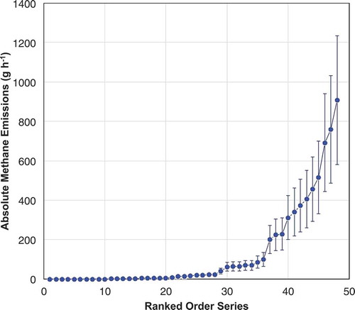
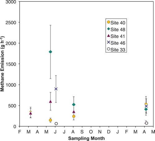
Figure 2. 13-month time series of CH₄ emissions from five wells where emission rates were measured more than once. Well numbers are as in Table 1 and Figure 1. Error bars represent the average standard deviation of all samples taken from the high-flow instrument of 36%.

Production data for the wells we sampled were taken from the ODNR production database and is shown in Table 1. Most wells produced only oil or gas, and a few produced both (Table 1), but all of the wells were listed as “producing” or “active” by ODNR, even if they had a production rate of 0 for 2018 (4 out of 48 wells in Table 1). Annual production of natural gas for 2018 (the most recent year available) for the wells visited ranges from 0 to 2584 MCF, with an average of 349 MCF. The annual production of oil ranges from 0 to 214 barrels for 2018, with an average of 30 barrels (“Oil & Gas Well Production Numbers,” 2020). Although ODNR maintains a vast archive of oil and gas records, there is a disclaimer on their oil and gas production database that does not guarantee the accuracy of the information provided. All of our wells are considered marginally producing wells, using the IRS definition of less than 15 barrels per day (5,475 barrels per year) for oil and 90 MCF per day (approximately 33,000 MCF annually) for gas production (Internal Revenue Service 2019; US Energy Information Administration 2018). All of the wells we sampled are in EIA’s lowest production rate bracket for marginal wells, 0−1 barrel of oil equivalent/well/day. This is the most abundant type of oil and gas well in the United States, with over 325,000 wells in 2018 (US Energy Information Administration 2018). In addition, wells producing between 0 and 1 BOE are the most abundant category of well in Ohio, making our results likely representative of the full population.

Methane emission quantification

Upon arrival, components at the wellhead and pumpjack such as joints, fittings, valves, and vents at each well were screened using a Bascom Turner Gas-Rover, which detects CH₄ enhancements above 10 ppm. We did not make measurements at gathering lines, separators, or tanks. In some cases, components such as valves and vents that appeared to be closed were emitting CH₄. Some oil producing wells had open vents, such as where a gas gathering line would otherwise be attached for natural gas collection or to vent annular gas. These vents were quantified, so our measurements include intentional vents as well as leaks. The number of emission sources quantified at each well is included in Table 1, as whether the well was venting or not, where noted in our field notes.

When a component with a CH₄ concentration over 500 ppm was identified with the screening instrument, the emission rate was subsequently measured using an Indaco Hi-Flow sampler (Townsend-Small et al. 2016). When a well had no components that screened above 500 ppm, this well was assigned an emission rate of 0 g hr⁻¹, similar to EPA method 21 (United States Code of Federal Regulations (US CFR) 2017) and as in our previous work (Townsend-Small et al. 2016).

High-flow sampling has been used across the oil and gas supply chain to measure CH₄ emissions (Brantley, Thoma, and Eisele 2015; Lamb et al. 2015; Townsend-Small et al. 2016). The high-flow sampling technique uses a high-flow rate of air and a loose enclosure to completely capture the gas emitting from a source. Due to the loose enclosure, emitted gas is mixed with background air. The sampler measures concentrations of background air and the mixed air plus emitted gas, as well as the flow of the sample (emitted gas plus background air). Methane emissions are calculated using Equation (1)(1) $\begin{array}{rl}& \mathrm{C}{\mathrm{H}}_4\mathrm{e}\mathrm{m}\mathrm{i}\mathrm{s}\mathrm{s}\mathrm{i}\mathrm{o}\mathrm{n}\mathrm{r}\mathrm{a}\mathrm{t}\mathrm{e}\left(\mathrm{k}\mathrm{g}/\mathrm{h}\right)=\mathrm{f}\mathrm{l}\mathrm{o}{\mathrm{w}}_{\mathrm{h}\mathrm{i}\mathrm{g}\mathrm{h}-\mathrm{f}\mathrm{l}\mathrm{o}\mathrm{w}\mathrm{s}\mathrm{a}\mathrm{m}\mathrm{p}\mathrm{l}\mathrm{e}\mathrm{r}}\\ & \mathrm{x}\left(\mathrm{c}\mathrm{o}\mathrm{n}\mathrm{c}\mathrm{e}\mathrm{n}\mathrm{t}\mathrm{r}\mathrm{a}\mathrm{t}\mathrm{i}\mathrm{o}{\mathrm{n}}_{\mathrm{s}\mathrm{a}\mathrm{m}\mathrm{p}\mathrm{l}\mathrm{e}}-\mathrm{c}\mathrm{o}\mathrm{n}\mathrm{c}\mathrm{e}\mathrm{n}\mathrm{t}\mathrm{r}\mathrm{a}\mathrm{t}\mathrm{i}\mathrm{o}{\mathrm{n}}_{\mathrm{b}\mathrm{a}\mathrm{c}\mathrm{k}\mathrm{g}\mathrm{r}\mathrm{o}\mathrm{u}\mathrm{n}\mathrm{d}}\right)\\ & /\mathrm{r}\mathrm{e}\mathrm{s}\mathrm{p}\mathrm{o}\mathrm{n}\mathrm{s}\mathrm{e}\mathrm{f}\mathrm{a}\mathrm{c}\mathrm{t}\mathrm{o}\mathrm{r}\end{array}$(1) , below. The Indaco device uses a vacuum pump, two Bascom Turner Gas Sentry instruments and a hot wire anemometer to measure the amount of CH₄ being emitted from each source (Howard, Ferrara, and Townsend-Small 2015; Lamb et al. 2015). One of the Gas Sentry instruments measures the CH₄ concentration of the sample plus background air, and the other measures the background air only (Howard, Ferrara, and Townsend-Small 2015). Photographs of the screening and emission rate quantification techniques are provided in the supplemental information.

When the inlet of the high-flow sampler was positioned on an emitting component, a tarp attached to the inlet was draped over the source of CH₄ and loosely tightened to ensure all the gas was routed into the measurement system. To ensure the high-flow sampler was positioned properly, the Gas-Rover was placed in the outlet of the high-flow sampler. This practice allows for the operator to compare the screening values and outflow values to further ensure an accurate measurement.

A series of three CH₄ samples were collected at each measurement point from the outlet of the high-flow sampler via syringe and transferred into evacuated glass vials. The samples collected were analyzed by gas chromatography-flame ionization detection (GC-FID) at the University of Cincinnati. The CH₄ concentrations measured by the GC-FID were used to calculate the CH₄ emission rate at each emitting component. This method was chosen because both the Gas Rover and the Gas Sentry are designed to measure CH₄ in high CH₄ concentration environments, such as distribution pipelines, and not in production gas environments where there are other hydrocarbons present. Sensors in these instruments have unknown response factors from non-methane hydrocarbons which make it difficult to correct the CH₄ concentrations measured by the Gas Rover and the high-flow (Connolly, Robinson, and Gardiner 2019; Howard, Ferrara, and Townsend-Small 2015). The GC-FID provides a concentration measurement for CH₄ only.

The CH₄ detectors on the Gas Rover and the high-flow sampler were calibrated daily on each day of use, using standards of 2.5% CH₄ and 100% CH₄. The flow velocity sensor on the high-flow sampler was also calibrated daily during use, using a four or five point calibration curve. Samples on the GC-FID were analyzed with bracketed standards, ranging from sub-atmospheric concentrations to 95% CH₄.

Whole-air samples

An additional focus of this study was to measure the emission rate of VOCs from marginal oil and gas wells. We took whole air samples at a subset of sampling sites (n = 16) to determine the emission rate of VOCs that are known hazardous air pollutants (HAPs). 1–3 L evacuated stainless steel canisters without flow regulators were positioned to take samples in the outlet of the high-flow sampler (in the same location as the CH₄ sample collection) during emission rate measurement (Brantley, Thoma, and Eisele 2015). These samples were collected in conjunction with a CH₄ sample from the outlet of the high-flow sampler to establish a VOC:CH₄ ratio. This method provides a measurement with the assumption of no losses of VOCs throughout the sampler during passage through the sampler. Whole air samples were taken at the component with the highest screening value at each well. The whole air samples were analyzed according to EPA method TO-15. VOCs in ambient air including a variety of VOCs related to the oil and gas industry, such as the BTEX compounds, hexane, cyclohexane, and heptane (United States Environmental Protection Agency 1999). HAPs are defined by the U.S. Environmental Protection Agency as air pollutants that can cause cancer or have other impacts on human health. They may also be referred to as air toxics or toxic air pollutants (EPA 2017; US EPA 2015).

Data analysis

CH₄ emissions were calculated using Equation 1(1) $\begin{array}{rl}& \mathrm{C}{\mathrm{H}}_4\mathrm{e}\mathrm{m}\mathrm{i}\mathrm{s}\mathrm{s}\mathrm{i}\mathrm{o}\mathrm{n}\mathrm{r}\mathrm{a}\mathrm{t}\mathrm{e}\left(\mathrm{k}\mathrm{g}/\mathrm{h}\right)=\mathrm{f}\mathrm{l}\mathrm{o}{\mathrm{w}}_{\mathrm{h}\mathrm{i}\mathrm{g}\mathrm{h}-\mathrm{f}\mathrm{l}\mathrm{o}\mathrm{w}\mathrm{s}\mathrm{a}\mathrm{m}\mathrm{p}\mathrm{l}\mathrm{e}\mathrm{r}}\\ & \mathrm{x}\left(\mathrm{c}\mathrm{o}\mathrm{n}\mathrm{c}\mathrm{e}\mathrm{n}\mathrm{t}\mathrm{r}\mathrm{a}\mathrm{t}\mathrm{i}\mathrm{o}{\mathrm{n}}_{\mathrm{s}\mathrm{a}\mathrm{m}\mathrm{p}\mathrm{l}\mathrm{e}}-\mathrm{c}\mathrm{o}\mathrm{n}\mathrm{c}\mathrm{e}\mathrm{n}\mathrm{t}\mathrm{r}\mathrm{a}\mathrm{t}\mathrm{i}\mathrm{o}{\mathrm{n}}_{\mathrm{b}\mathrm{a}\mathrm{c}\mathrm{k}\mathrm{g}\mathrm{r}\mathrm{o}\mathrm{u}\mathrm{n}\mathrm{d}}\right)\\ & /\mathrm{r}\mathrm{e}\mathrm{s}\mathrm{p}\mathrm{o}\mathrm{n}\mathrm{s}\mathrm{e}\mathrm{f}\mathrm{a}\mathrm{c}\mathrm{t}\mathrm{o}\mathrm{r}\end{array}$(1) (Howard, Ferrara, and Townsend-Small 2015)

(1) $\begin{array}{rl}& \mathrm{C}{\mathrm{H}}_4\mathrm{e}\mathrm{m}\mathrm{i}\mathrm{s}\mathrm{s}\mathrm{i}\mathrm{o}\mathrm{n}\mathrm{r}\mathrm{a}\mathrm{t}\mathrm{e}\left(\mathrm{k}\mathrm{g}/\mathrm{h}\right)=\mathrm{f}\mathrm{l}\mathrm{o}{\mathrm{w}}_{\mathrm{h}\mathrm{i}\mathrm{g}\mathrm{h}-\mathrm{f}\mathrm{l}\mathrm{o}\mathrm{w}\mathrm{s}\mathrm{a}\mathrm{m}\mathrm{p}\mathrm{l}\mathrm{e}\mathrm{r}}\\ & \mathrm{x}\left(\mathrm{c}\mathrm{o}\mathrm{n}\mathrm{c}\mathrm{e}\mathrm{n}\mathrm{t}\mathrm{r}\mathrm{a}\mathrm{t}\mathrm{i}\mathrm{o}{\mathrm{n}}_{\mathrm{s}\mathrm{a}\mathrm{m}\mathrm{p}\mathrm{l}\mathrm{e}}-\mathrm{c}\mathrm{o}\mathrm{n}\mathrm{c}\mathrm{e}\mathrm{n}\mathrm{t}\mathrm{r}\mathrm{a}\mathrm{t}\mathrm{i}\mathrm{o}{\mathrm{n}}_{\mathrm{b}\mathrm{a}\mathrm{c}\mathrm{k}\mathrm{g}\mathrm{r}\mathrm{o}\mathrm{u}\mathrm{n}\mathrm{d}}\right)\\ & /\mathrm{r}\mathrm{e}\mathrm{s}\mathrm{p}\mathrm{o}\mathrm{n}\mathrm{s}\mathrm{e}\mathrm{f}\mathrm{a}\mathrm{c}\mathrm{t}\mathrm{o}\mathrm{r}\end{array}$(1)

For this study, the value used for sample concentration was the concentration of CH₄ measured with GC-FID. The background concentration was measured by the Gas Sentry instrument in the high-flow sampler. Since CH₄ samples for GC analysis were taken at every measurement point, the response factor was assumed to be 1 for the GC, which only measured CH₄ and not any other non-CH₄ hydrocarbons.

VOC emission rates were estimated using the concentrations of VOCs measured in the whole air samples. Each whole air sample was taken in conjunction with a CH₄ sample, allowing the use of a VOC:CH₄ ratio to estimate a VOC emission rate. Following the equation presented in (Marrero et al. 2016), emission rates for each HAP measured were calculated as in Equation 2(2) $\begin{array}{rl}& \mathrm{V}\mathrm{O}\mathrm{C}\mathrm{f}\mathrm{l}\mathrm{u}\mathrm{x}=\mathrm{C}{\mathrm{H}}_4\mathrm{f}\mathrm{l}\mathrm{u}\mathrm{x}\left(\mathrm{g}{\mathrm{h}}^{-1}\right)\\ & \ast \left(\mathrm{m}\mathrm{o}\mathrm{l}\mathrm{e}\mathrm{c}\mathrm{u}\mathrm{l}\mathrm{a}\mathrm{r}\mathrm{w}\mathrm{e}\mathrm{i}\mathrm{g}\mathrm{h}\mathrm{t}\mathrm{V}\mathrm{O}\mathrm{C}/\mathrm{m}\mathrm{o}\mathrm{l}\mathrm{e}\mathrm{c}\mathrm{u}\mathrm{l}\mathrm{a}\mathrm{r}\mathrm{w}\mathrm{e}\mathrm{i}\mathrm{g}\mathrm{h}\mathrm{t}\mathrm{C}{\mathrm{H}}_4\right)\\ & \ast \left(\left[\mathrm{V}\mathrm{O}\mathrm{C}\right]:\left[\mathrm{C}{\mathrm{H}}_4\right]\right)\end{array}$(2) .

(2) $\begin{array}{rl}& \mathrm{V}\mathrm{O}\mathrm{C}\mathrm{f}\mathrm{l}\mathrm{u}\mathrm{x}=\mathrm{C}{\mathrm{H}}_4\mathrm{f}\mathrm{l}\mathrm{u}\mathrm{x}\left(\mathrm{g}{\mathrm{h}}^{-1}\right)\\ & \ast \left(\mathrm{m}\mathrm{o}\mathrm{l}\mathrm{e}\mathrm{c}\mathrm{u}\mathrm{l}\mathrm{a}\mathrm{r}\mathrm{w}\mathrm{e}\mathrm{i}\mathrm{g}\mathrm{h}\mathrm{t}\mathrm{V}\mathrm{O}\mathrm{C}/\mathrm{m}\mathrm{o}\mathrm{l}\mathrm{e}\mathrm{c}\mathrm{u}\mathrm{l}\mathrm{a}\mathrm{r}\mathrm{w}\mathrm{e}\mathrm{i}\mathrm{g}\mathrm{h}\mathrm{t}\mathrm{C}{\mathrm{H}}_4\right)\\ & \ast \left(\left[\mathrm{V}\mathrm{O}\mathrm{C}\right]:\left[\mathrm{C}{\mathrm{H}}_4\right]\right)\end{array}$(2)

Because the TO-15 method analyzes for a variety of VOCs, the emission rates of each VOC detected in the whole air samples were calculated separately.

Production rates were obtained through the ODNR production database in order to calculate gas production-normalized emissions and assess the ratio of natural gas lost at each well. We took samples and measured the composition of wellhead gas in seven wells in the Wayne National Forest and used these data to convert the natural gas production rate to CH₄ production rate. The average gas composition for wells in the Marietta section was 78.4% CH₄ and the average gas composition for wells in the Athens section was 85.5% CH₄.

Error analysis

Each component was measured a total of three times during each visit. The error in our study-wide CH₄ emission rate measurement was estimated by averaging the standard deviation of the three CH₄ measurements with the mean emission rate for each measurement, for an average error of 36%.

Results and discussion

Methane emissions from marginal wells

Methane emissions from marginal wells measured in our study are shown in Figure 1. The error bars represent the average normalized standard deviation of the CH₄ emission rates derived from the CH₄ samples taken from the outflow of the high-flow sampler. We found a skewed distribution of CH₄ emission rates, indicating that only few of the wells measured are responsible for a majority of the emissions. Many of the wells (n = 22 out of 48) emitted 10 g h⁻¹ or less. Twenty-seven percent (n = 13) of the wells measured emitted over 100 g h⁻¹. The emission rates ranged from 0 g h⁻¹ to 907 g h⁻¹ with an average emission rate of 128 g h⁻¹ and a median emission rate of 18 g h⁻¹. The top four highest emitters, or 8% of the wells measured, were responsible for approximately 50% of the total CH₄ emissions observed in the study. This pattern of skewed distribution of CH₄ emissions has been found in previous studies of abandoned wells (Townsend-Small et al. 2016) as well as one previous study of active conventional wells (Omara et al. 2016) in the Appalachian Basin, and is characteristic of all natural gas systems nationally (Zavala-Araiza et al. 2015). The highest emitter in this study had an average emission rate of 906.7 g h⁻¹. The wellhead had been damaged by a fallen tree, the natural gas gathering line was not present, and a valve was opened to vent the natural gas being produced. This well was measured three times over the course of the study (see further discussion below).

The average CH₄ emission rate for marginal wells in this study was in the same order of magnitude as other conventional wells in Appalachia. Marginally producing conventional gas wells in Pennsylvania and West Virginia had an average emission rate of 820 g h⁻¹ (Omara et al. 2016); higher than our wells, although the wells in the current study had much lower oil and gas production rates than those measured by (Omara et al. 2016). The study by (Omara et al. 2016) used site-level measurement techniques that would include emissions from tanks, which we did not measure, and our results should be considered conservative for that reason. Our results are similar to the average emission rate of conventional oil and gas wells in West Virginia of 138 g h⁻¹, with production normalized emissions ranging from 0.02% to 56% from wells with an average gas production rate of 33,387 kg yr⁻¹ (Riddick et al. 2019). Although the wells we measured had the lowest rates of production nationally, and most were producing only oil or gas and not both, they had much higher CH₄ emission rates than abandoned wells. Unplugged abandoned wells in Appalachian Ohio emit CH₄ at an average emission rate of 28 g h⁻¹ (Townsend-Small et al. 2016). This is similar to the average emission rate for abandoned wells in Pennsylvania of 11 g h⁻¹ (Kang et al. 2014).

It is complicated to directly compare our results to measurements from higher producing hydraulic fracturing wells, because so many of our wells may be venting natural gas, whereas previous studies have been from hydraulic fracturing wells that are producing gas to pipelines. However, emission rates from marginal wells were lower than those reported from hydraulic fracturing wells. Unconventional wells in the Marcellus Shale were emitting CH₄ at an average of 18,800 g hr⁻¹, and at a much smaller proportion of production than conventional wells (0.01– 1.2%) (Omara et al. 2016). A study of wells in the Barnett Shale found average emission rates of 630 g hr⁻¹ (Rella et al. 2015). Hydraulic fracturing wells in the Barnett, Denver-Julesburg, and Pinedale Basins had average emission rates of 1200, 504, and 2124 g hr⁻¹, respectively (Brantley et al. 2014).

The United States EPA developed an emission factor for active marginal wells based on model wells from a previous study of unconventional wells (Brantley et al. 2014). EPA estimates that marginal gas wells emit 4.8 tons of CH₄ per year (548 g CH₄ hr⁻¹) and that marginal oil wells emit 1.83 tons CH₄ per year (208 g CH₄ hr⁻¹) (United States Environmental Protection Agency 2018). ODNR does not distinguish between oil versus gas wells, but our average CH₄ emission rates were not different between wells that did and did not report an oil production rate for 2018. Our study sites are at the very lowest end of production rates for active wells nationally (0–1 BOE d⁻¹), whereas we assume that the EPA emission factor represents the entire production range of marginal wells (0–15 BOE d⁻¹), so this comparison is not straightforward. More field studies are needed to quantify CH₄ emission factors from the full production range of marginal wells.

Relationship with gas production

Previous studies in this region have shown that CH₄ emissions from natural gas wells have a predictable, positive relationship with gas production (Omara et al. 2016; Riddick et al. 2019). This relationship has also been used to scale national CH₄ emission rates from the production sector, including both conventional and unconventional wells (Alvarez et al. 2018; Omara et al. 2018). A recent synthesis including new data indicated that while newer, higher producing wells are a major source of CH₄ nationally, marginal wells may emit a much higher proportion of the gas produced (Omara et al. 2018). In the current study, out of the 48 wells visited, only 25 produced natural gas in 2018 according to the ODNR database, and the rest were either oil wells with a reported production rate of 0 for natural gas, or had no oil or gas production in 2018 (Table 1).

To explore the relationship between CH₄ emissions and natural gas production rates, we calculated production normalized emissions using the CH₄ emissions we measured in the field and annual natural gas production data for 2018 obtained from the ODNR production database (“Oil & Gas Well Production Numbers,” 2020). After correcting for CH₄ composition of natural gas, the overall mean CH₄ production rate for our wells was 612 g hr⁻¹, including wells with zero production. Using this average production rate, we can calculate a weighted average for all wells of total CH₄ emitted divided by total CH₄ produced of 21%. For wells with non-zero gas production rates (i.e., gas or oil and gas wells), the average production normalized emission rate was 117% (median: 2%, range: 0%-2434%). Two wells had production normalized emissions greater than 100%: one well had a CH₄ emission rate of 515 g h⁻¹ and an annual production rate of 131 MCF for 2018, for a normalized production rate of 229% (Table 1). Another well had a CH₄ emission rate of 455 g h⁻¹ and an annual production rate of 10 MCF for 2018, for a normalized production rate of 2434% (Table 1). Without these two outliers, the average production normalized emission rate for gas wells was 7%. We also had 21 wells where we found a positive CH₄ emission rate and no recorded natural gas production for 2018 (i.e., oil wells). This includes our highest emitting well in the entire study (Table 1). These wells had a CH₄ emission rate ranging from 0.1 to 907 g h⁻¹. No production normalized emission rate can be calculated for these wells; a production normalized rate of >100% is assigned in Table 1. Finally, we also had four wells where we found no emissions and there was no gas production reported for 2018 in the ODNR database; for these wells, we assigned a production normalized emission rate of 0%.

Both of the previous studies of low producing conventional wells in Appalachia found a positive relationship between production rate and CH₄ emissions. A study conducted in West Virginia sampled at 74 wells but was only able to gather gas production data for 25 of them. Their average production normalized emission rate was 8.8% (range: 0.02–56%) (Riddick et al. 2019). Another study conducted in Pennsylvania and West Virginia found similar results to Riddick et al., with a median of 10.5% and range of 0.35–91% (Omara et al. 2016). Neither of these studies found CH₄ emissions that were greater than reported gas production at any well. Unlike in the previous studies, there was no correlation between the CH₄ emissions and annual production in our data, with many zero production numbers in our database (R² = 0.003). Because our wells had such low production rates, and many of our wells were found to be emitting more gas than producing and leaking oil (Table 1), the production rate data are somewhat less meaningful than for higher producing wells. Because of this, our “production normalized” emission rates should be interpreted with caution, as clearly the state production data do not represent all of the oil and gas coming from these wells.

We propose that the main driver of emissions from the wells visited is neglect. The state of maintenance at these wells was poor. Often, pumpjacks, tanks, and other infrastructure were rusty and sometimes appeared to have temporary fixes to just keep the well mechanically operational. When we noted maintenance problems at sampling sites, these are described in Table 1. Some wells looked like they had not been serviced in years. Sometimes, leaks were found at fittings and joints. We also found several wells with open valves that appeared to be for natural gas gathering lines. One well had a ~1 inch diameter hole in the casing near the base of the wellhead. Two of the wells had trees that had fallen on the wellhead. In other cases, emissions were detectable via sight or smell at wellheads. Oil was sometimes present spilled on the ground or around well casings. Maintenance status had a significant effect on CH₄ emissions in our study (p = .04). At wells where poor maintenance was noted, the average CH₄ emission rate was 183 g h⁻¹, whereas at wells were we noted maintenance was good or no maintenance status was noted, the average CH₄ emission rate was 50 g h⁻¹ (see Table 1 for a description of maintenance at all study sites). While we note that our study did not aim to collect maintenance data at each well, and thus these calculations should be considered preliminary, the effect of maintenance status on CH₄ emissions, as well as the fact that many wells are venting gas and leaking oil (Table 1) may suggest that these wells are producing just enough oil or gas to keep them in the “active” category and forestall permanent abandonment, which requires expensive plugging within a certain amount of time. On the other hand, these wells may provide a minor but critical and steady amount of income to small operators in Appalachia, helped with tax offsets.

Are methane emissions episodic?

Most previous studies of CH₄ emissions from production sites have been based on single measurements, leading to questions about whether high emitters represent episodic events. In order to address this question, we visited some wells multiple times to assess whether CH₄ emissions are changing significantly over time. Figure 2 shows CH₄ emissions of five wells sampled between two and five times over 13 months. The error bars represent the average normalized standard deviation of all samples of 36%. We observed variation in CH₄ emissions over the study period, however, at no well did we observe an emission that appeared to be a one-time event. At some wells, CH₄ emissions decreased over time, including at our highest emitter, well 48, as well as at well 46 (Figure 2). At other sites, the emission rate varied overtime or increased (Figure 2).

The well with the largest decrease in emission rate was the largest emitter in our study (well 48, Figure 2, Table 1). This was the well-described above with the fallen tree on the wellhead and the open gathering line. In our second sampling visit (August 2018), we observed the tree had been cleared away, indicating at least some maintenance had been done on the well, but the open gathering line was still audibly emitting. Decreasing reservoir pressure due to venting may also be responsible for the decrease in emission rate observed at this well between the first and second measurement. Other wells did not exhibit significant differences in emission rate between measurements. Environmental conditions such as temperature and pressure were incorporated into the flow calibration for the quantification of CH₄ emissions. Wind speed was addressed by isolating emissions with a plastic tarp.

Volatile organic carbon emissions

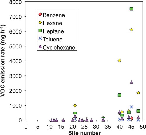
Figure 3 shows the distribution of VOC emissions for the top five VOCs emitted. Emission rates are also shown in Table 2, with the full suite of VOCs identified in the study found in Table S1. As with CH₄ emissions, there is a skewed distribution of VOCs with a few wells representing the majority of emissions (Figure 3). Hexane and heptane were the most abundantly emitted VOCs, with average emission rates of 902 and 704 mg h⁻¹, respectively (Figure 3, Table 2). This was followed by cyclohexane, toluene, and benzene, with average emission rates of 246, 68, and 50 mg h⁻¹, respectively (Figure 3). Emission rates of VOCs did not follow the same distribution of CH₄ emissions, as the highest CH₄ emitter, well 48, was not the highest emitter of VOCs (Figure 3). As seen in Figure 3, each gas well had a different VOC emission profile. As with CH₄ emissions, we also did not see a relationship of VOC emissions with oil or gas production rate.

Table 2. Range of VOC emissions found in the current study. Well numbers are the same as in Table 1. Top five most abundantly emitted VOCs are shown. Data are also shown in Figure 3. The full suite of VOC emissions found in this study can be found in Table S1.

Well number	Benzene Emission Rate (mg h^−1)	Hexane Emission Rate (mg h^−1)	Heptane Emission Rate (mg h^−1)	Toluene Emission Rate (mg h^−1)	Cyclohexane Emission Rate (mg h^−1)
11	0	0	1	0	0
12	0	1	1	0	0
13	0	3	1	0	0
16	1	16	7	0	2
20	0	4	10	0	17
21	25	970	446	51	264
23	1	49	18	2	10
24	0	22	11	1	4
26	3	75	33	2	27
28	0	8	3	0	2
33	1	145	80	1	18
40	492	4021	1683	69	550
41	28	554	299	29	127
44	25	617	533	35	210
45	134	6117	7526	884	2564
48	92	1830	619	13	195

Figure 3. Emission rate of the five most abundantly emitted VOCs (mg h⁻¹). Well numbers are the same as in Table 1 and Figure 1.

Other studies have measured VOC emission rates from unconventional oil and gas wells and found higher rates of VOC emissions, although these wells are also larger sources of CH₄ and produce oil and gas at rates many orders of magnitude larger than the ones in the current study. For example, the average benzene flux from individual unconventional wells in the Barnett Shale was 4.9 g h⁻¹ (Marrero et al. 2016), compared to an average flux from marginal wells in the current study of 50 mg h⁻¹ (Table 2). However, similar to the current study, the most abundantly emitted VOC from wells in the Barnett Shale was hexane (Marrero et al. 2016). Unconventional wells in the Denver-Julesburg Basin also emit VOCs at higher rates than marginal wells, from 72 to 8352 g h⁻¹ (Brantley, Thoma, and Eisele 2015). The whole air samples collected in this study were tested for several PAHs, however, none were detectable, unlike in previous studies that sampled adjacent to unconventional wells in Ohio (Paulik et al. 2016).

Despite the relatively low emission rates found here, these sources may still pose a significant risk to those exposed, especially if marginal wells are on or near residential property and lead to long-term exposure; a particular danger given the large number of marginal wells in Appalachia and nationwide. For example, proximity to low producing and inactive wells in urban areas can affect birth outcomes in pregnant women (Tran et al. 2020). Holes in well casings, as noted in a few cases in Table 1, could lead to aquifer contamination: an additional hydrocarbon exposure pathway for residents of rural areas who rely on groundwater as their only water source (Botner et al. 2018; Osborn et al. 2011). We also noted some wellheads where brine appeared to have spilled from vents, which could pose a hazard to human and ecosystem health. Another serious consequence of our results is for oil and gas field workers, who will be exposed to high levels of VOCs at wells that are venting. Although we observed at least two wells where vents were routed up above inhalation level using tubing, in other cases, venting was at ground level or on the wellhead (Table 1). Acute exposure to VOCs can cause serious harm in oilfield workers, including sudden death (Harrison et al. 2016). These high emitting wells also present an explosion risk to workers.

Some VOCs and HAPs, like benzene and the other BTEX compounds, can lead to chronic diseases such as leukemia and other cancers, neurological damage, birth defects, and hearing loss (Garcia-Gonzalez et al. 2019; McKenzie et al. 2012). In this study, the most abundant HAPs measured were heptane and hexane. Inhalation of hexane, for example, can cause neuropathy and other neurological effects (US EPA 2013). Acute exposure of heptane can lead to dizziness, nausea, and dermatitis, among other symptoms (CDC 2018). Emissions of VOCs from marginal wells may also impact human health indirectly through the formation of tropospheric ozone (Pekney et al. 2014). The level of risk from these marginal wells would depend on the ambient concentration and the exposure time, as well as the emission rate of the toxic chemical from the well in question. As previously noted, the highest risk may be to workers who routinely come in close contact with high emitting wells (Esswein et al. 2014; Goldstein et al. 2014; Harrison et al. 2016).

Policy implications

Marginal natural gas wells on federal land in Ohio are emitting a significant portion of natural gas produced, and many oil wells are venting 100% of natural gas produced. There are hundreds of thousands of these marginal “stripper” wells in the United States. The results of this study indicate that, despite the lower absolute emission rates we have found relative to unconventional wells, these marginal wells may be a nationally significant source of CH₄. Scaling our results to a national level is a challenge. Previous studies have used the relationship of CH₄ emission rate with gas production for scaling-up, but we found no such relationship. We also found no relationship of CH₄ emissions with well age. Multiplying our average emission factor for marginal wells in the 0 −1 BOE well⁻¹ d⁻¹ category by the total number of wells in this category (336,012 in 2018) (US Energy Information Administration 2018) gives an annual emission rate of 0.4 ± 0.1 Tg CH₄ yr⁻¹: this is about 11% of total CH₄ emissions from oil and gas production in the EPA GHG inventory and 5% of CH₄ emissions from the production sector in a recent synthesis of measurement campaigns (Alvarez et al. 2018). According to EIA, marginal wells in the 0–1 BOE d⁻¹ category produced only 0.2% of annual oil production and 0.4% of annual natural gas production in 2018 (US Energy Information Administration 2018), indicating that wells in this category are a disproportionate source of CH₄. Future work may consider measurements in additional production rate brackets and regions to create national emissions factors (US Energy Information Administration 2018), as well as measurements from oil storage tanks at marginal wells, as these tanks may have similar maintenance issues to those noted at wellheads.

Mitigating emissions from just one category of stripper wells (0–1 BOE d⁻¹) could reduce CH₄ emissions from the oil and gas supply chain by up to 5% to 10% with an extremely minor impact on domestic energy supply. This shortfall in oil and gas supply could be eliminated by drilling a much smaller number of new unconventional wells, which emit CH₄ at lower proportions (Omara et al. 2016). There may be a large number of stripper wells on public land, and these could be a preliminary target for mitigation, with concomitant air quality and recreational benefits (Pekney et al. 2014; Ratledge, Davis, and Zachary 2019). Regular maintenance may be one way to prevent the loss of natural gas and emissions of VOCs from marginal wells. Regulation of marginal wells such as leak detection and repair or requiring flaring instead of venting may help mitigate emissions. Over the past decade, the contribution of marginal wells to regional and national oil and natural gas supply chains has sharply declined (US Energy Information Administration 2018); therefore, another mitigation pathway for these emissions may be permanent plugging, which sharply decreases CH₄ and VOC emissions (Townsend-Small et al. 2016) and may also create jobs. Because these emissions may be relatively easy to mitigate and may represent a substantial portion of national emissions from oil and gas production, this is an important area for future research and regulation.

Acknowledgment

The authors thank Edwin Barth and Daniel Sturmer for supportive comments on the manuscript draft, Anastasia Fries and Julianne Fernandez for assistance with field and laboratory work, David Lyon with assistance with database access, and Tom Ferrara for assistance with equipment and many other technical and scientific aspects of the study. The manuscript was significantly improved with the help of three anonymous reviewers. TO-15 whole air samples were processed and analyzed by ALS Environmental Services in Blue Ash, Ohio, and wellhead gas samples were analyzed by PACE Analytical Services. The authors declare no competing financial interests.

Disclosure statement

No potential conflict of interest was reported by the authors.

Supplementary material

Supplemental data for this paper can be accessed on the publisher’s website.

Additional information

Funding

This work was funded by a grant from the Bureau of Land Management, United States Department of Interior (Grant number L17AC00015). Additional funding was provided by the University of Cincinnati Women in Science and Engineering program.

Notes on contributors

Jacob A. Deighton

Jacob A. Deighton was an M.S. student in Geology at the University of Cincinnati. He is an environmental scientist with a background in air quality research.

Amy Townsend-Small

Amy Townsend-Small is an Associate Professor in the Department of Geology at University of Cincinnati. She can be contacted at [email protected].

Sarah J. Sturmer

Sarah J. Sturmer was a lab manager in Geology at University of Cincinnati. She is currently an adjunct professor of Environmental Studies at University of Cincinnati and of Geology at Southern New Hampshire University.

Jacob Hoschouer

Jacob Hoschouer is pursuing a B.S. in Environmental Studies at the University of Cincinnati with an interest in air quality.

Laura Heldman

Laura Heldman is in her senior year at the University of Cincinnati pursuring a B.S. in Environmental Studies. She plans to continue her studies in the field of environmental law.

References

- Alvarez, R. A., D. Zavala-Araiza, D. R. Lyon, D. T. Allen, Z. R. Barkley, A. R. Brandt, K. J. Davis, S. C. Herndon, D. J. Jacob, A. Karion, et al. 2018. Assessment of methane emissions from the U.S. oil and gas supply chain. Science eaar7204. doi:10.1126/science.aar7204.
- Botner, E. C., A. Townsend-Small, D. B. Nash, X. Xu, A. Schimmelmann, and J. H. Miller. 2018. Monitoring concentration and isotopic composition of methane in groundwater in the Utica Shale hydraulic fracturing region of Ohio. Environ. Monit. Assess. 190:322. doi:10.1007/s10661-018-6696-1.
- Brandt, A. R., G. A. Heath, E. A. Kort, F. O’Sullivan, G. Pétron, S. M. Jordaan, P. Tans, J. Wilcox, A. M. Gopstein, D. Arent, et al. 2014. Methane leaks from North American natural gas systems. Science 343:733–35. doi:10.1126/science.1247045.
- Brantley, H. L., E. D. Thoma, and A. P. Eisele. 2015. Assessment of volatile organic compound and hazardous air pollutant emissions from oil and natural gas well pads using mobile remote and on-site direct measurements. J. Air Waste Manag. Assoc. 65:1072–82. doi:10.1080/10962247.2015.1056888.
- Brantley, H. L., E. D. Thoma, W. C. Squier, B. B. Guven, and D. Lyon. 2014. Assessment of methane emissions from oil and gas production pads using mobile measurements. Environ. Sci. Technol. 48:14508–15. doi:10.1021/es503070q.
- CDC. 2018. NIOSH pocket guide to chemical hazards - n-heptane [WWW Document]. Cent. Dis. Control Prev. Accessed April 15, 2020. https://www.cdc.gov/niosh/npg/npgd0312.html.
- Connolly, J. I., R. A. Robinson, and T. D. Gardiner. 2019. Assessment of the Bacharach Hi Flow® Sampler characteristics and potential failure modes when measuring methane emissions. Measurement 145:226–33. doi:10.1016/j.measurement.2019.05.055.
- Elliott, E. G., X. Ma, B. P. Leaderer, L. A. McKay, C. J. Pedersen, C. Wang, C. J. Gerber, T. J. Wright, A. J. Sumner, M. Brennan, et al. 2018. A community-based evaluation of proximity to unconventional oil and gas wells, drinking water contaminants, and health symptoms in Ohio. Environ. Res. 167:550–57. doi:10.1016/j.envres.2018.08.022.
- Esswein, E. J., J. Snawder, B. King, M. Breitenstein, M. Alexander-Scott, and M. Keifer. 2014. Evaluation of some potential chemical exposure risks during flowback operations in unconventional oil and gas extraction: Preliminary results. J. Occup. Environ. Hyg. 11:D174–D184. doi:10.1080/15459624.2014.933960.
- Garcia-Gonzalez, D. A., S. A. Shonkoff, J. Hays, and M. Jerrett. 2019. Hazardous air pollutants associated with upstream oil and natural gas development: A critical synthesis of current peer-reviewed literature. Annu. Rev. Public Health 40:283–304. doi:10.1146/annurev-publhealth-040218-043715.
- Goldstein, B. D., B. W. Brooks, S. D. Cohen, A. E. Gates, M. E. Honeycutt, J. B. Morris, J. Orme-Zavaleta, T. M. Penning, and J. Snawder. 2014. The role of toxicological science in meeting the challenges and opportunities of hydraulic fracturing. Toxicol. Sci. 139:271–83. doi:10.1093/toxsci/kfu061.
- Harrison, R. J., K. Retzer, M. J. Kosnett, M. Hodgson, T. Jordan, S. Ridl, and M. Kiefer. 2016. Sudden deaths among oil and gas extraction workers resulting from oxygen deficiency and inhalation of hydrocarbon gases and vapors - United States, January 2010-March 2015. Morb. Mortal. Wkly. Rep. 65:6–9. doi:10.15585/mmwr.mm6501a2.
- Howard, T., T. W. Ferrara, and A. Townsend-Small. 2015. Sensor transition failure in the high flow sampler: Implications for methane emission inventories of natural gas infrastructure. J. Air Waste Manag. Assoc. 65:856–62. doi:10.1080/10962247.2015.1025925.
- Internal Revenue Service. 2019. 26 U.S. Code § 613A [WWW Document]. LII Leg. Inf. Inst. Accessed April 9, 2020. https://www.law.cornell.edu/uscode/text/26/613A.
- Kang, M., C. M. Kanno, M. C. Reid, X. Zhang, D. L. Mauzerall, M. A. Celia, Y. Chen, and T. C. Onstott. 2014. Direct measurements of methane emissions from abandoned oil and gas wells in Pennsylvania. Proc. Natl. Acad. Sci. 111:18173–77. doi:10.1073/pnas.1408315111.
- Lamb, B. K., S. L. Edburg, T. W. Ferrara, T. Howard, M. R. Harrison, C. E. Kolb, A. Townsend-Small, W. Dyck, A. Possolo, and J. R. Whetstone. 2015. Direct measurements show decreasing methane emissions from natural gas local distribution systems in the United States. Environ. Sci. Technol. 49:5161–69. doi:10.1021/es505116p.
- Marrero, J. E., A. Townsend-Small, D. R. Lyon, T. R. Tsai, S. Meinardi, and D. R. Blake. 2016. Estimating emissions of toxic hydrocarbons from natural gas production sites in the Barnett Shale region of Northern Texas. Environ. Sci. Technol. 50:10756–64. doi:10.1021/acs.est.6b02827.
- McKenzie, L. M., R. Z. Witter, L. S. Newman, and J. L. Adgate. 2012. Human health risk assessment of air emissions from development of unconventional natural gas resources. Sci. Total Environ. 424:79–87. doi:10.1016/j.scitotenv.2012.02.018.
- ODNR Oil & Gas Well Viewer. 2019. [WWW Document]. Accessed May 29, 2019. https://gis.ohiodnr.gov/MapViewer/?config=oilgaswells.
- Ohio Division of Geological Survey. 2004. Oil and Gas Fields Map of Ohio. Columbus, OH: Ohio Division of Natural Resources, Division of Geological Survey.
- Oil & Gas Well Production Numbers [WWW Document]. 2020. Accessed April 11, 2020. http://oilandgas.ohiodnr.gov/production.
- Omara, M., M. R. Sullivan, X. Li, R. Subramanian, A. L. Robinson, and A. A. Presto. 2016. Methane emissions from conventional and unconventional natural gas production sites in the Marcellus Shale Basin. Environ. Sci. Technol. 50:2099–107. doi:10.1021/acs.est.5b05503.
- Omara, M., N. Zimmerman, M. R. Sullivan, X. Li, A. Ellis, R. Cesa, R. Subramanian, A. A. Presto, and A. L. Robinson. 2018. Methane emissions from natural gas production sites in the United States: Data synthesis and national estimate. Environ. Sci. Technol. 52:12915–25. doi:10.1021/acs.est.8b03535.
- Osborn, S. G., A. Vengosh, N. R. Warner, and R. B. Jackson. 2011. Methane contamination of drinking water accompanying gas-well drilling and hydraulic fracturing. Proc. Natl. Acad. Sci. 108:8172–76. doi:10.1073/pnas.1100682108.
- Paulik, L. B., C. E. Donald, B. W. Smith, L. G. Tidwell, K. A. Hobbie, L. Kincl, E. N. Haynes, and K. A. Anderson. 2016. Emissions of polycyclic aromatic hydrocarbons from natural gas extraction into air. Environ. Sci. Technol. 50:7921–29. doi:10.1021/acs.est.6b02762.
- Pekney, N. J., G. Veloski, M. Reeder, J. Tamilia, E. Rupp, and A. Wetzel. 2014. Measurement of atmospheric pollutants associated with oil and natural gas exploration and production activity in Pennsylvania’s Allegheny National Forest. J. Air Waste Manag. Assoc. 64:1062–72. doi:10.1080/10962247.2014.897270.
- Potter, K., D. Shirley, I. Manos, and K. Muraoka. 2017. Tax credits and incentives for oil & gas producers in a low-price environment. J. Multistate Tax. Incent. 27:31–35.
- Ratledge, N., S. J. Davis, and L. Zachary. 2019. Public lands fly under climate radar. Nat. Clim. Change 9:92. doi:10.1038/s41558-019-0399-7.
- Rella, C. W., T. R. Tsai, C. G. Botkin, E. R. Crosson, and D. Steele. 2015. Measuring emissions from oil and natural gas well Pads using the mobile flux plane technique. Environ. Sci. Technol. 49:4742–48. doi:10.1021/acs.est.5b00099.
- Riddick, S. N., D. L. Mauzerall, M. A. Celia, M. Kang, K. Bressler, C. Chu, and C. D. Gum. 2019. Measuring methane emissions from abandoned and active oil and gas wells in West Virginia. Sci. Total Environ. 651:1849–56. doi:10.1016/j.scitotenv.2018.10.082.
- Townsend-Small, A., T. W. Ferrara, D. R. Lyon, A. E. Fries, and B. K. Lamb. 2016. Emissions of coalbed and natural gas methane from abandoned oil and gas wells in the United States. Geophys. Res. Lett. 43:2283–90. doi:10.1002/2015GL067623.
- Tran, K., J. Casey, L. Cushing, and R. Morello-Frosch. 2020. Residential proximity to oil and gas development and birth outcomes in California: A retrospective cohort study of 2006-2015 births. Environ. Health Perspect. 128. doi:org/doi:10.1289/EHP5842.
- U.S. Energy Information Administration. 2017. Appalachia region drives growth in U.S. natural gas production since 2012 - Today in Energy [WWW Document]. Accessed May 1, 2019. https://www.eia.gov/todayinenergy/detail.php?id=33972.
- United States Code of Federal Regulations (US CFR). 2017. Standards of performance for new stationary sources, Appendix A-7, Method 21 - Determination of volatile organic compound leaks (No. 40 CFR Part 60). Washington, DC: The United States Government.
- United States Environmental Protection Agency. 1999. Compendium of Methods for the Determination of Toxic Organic Compounds in Ambient Air, Second Edition, Compendium Method TO-15: Determination of Volatile Organic Compounds (VOCs) in Air Collected in Specially-Prepared Canisters and Analyzed by Gas Chromatography/Mass Spectrometry (GC/MS). Cincinnati, OH: USEPA Center for Environmental Research Information.
- United States Environmental Protection Agency. 2008. Polycyclic Aromatic Hydrocarbons (PAHs). Washington, DC: USEPA Office of Solid Waste.
- United States Environmental Protection Agency. 2018. Oil and natural gas sector: Emission standards for new, reconstructed, and modified sources. Background Technical Support Document for the Proposed Reconsideration of the New Source Performance Standards. 40 CFR Part 60, subpart OOOOa. Research Triangle Park, NC: USEPA Office of Air Quality Planning and Standards.
- US Energy Information Administration. 2018. The distribution of U.S. oil and natural gas wells by production rate. U.S. Department of Energy, Office of Independent Statistics and Analysis.
- US EPA. 2013. Integrated risk information system [WWW document]. US EPA. Accessed April 15, 2020. https://www.epa.gov/iris.
- US EPA. 2015. Hazardous air pollutants [WWW document]. US EPA. Accessed May 1, 2019. https://www.epa.gov/haps.
- US EPA. 2017. Inventory of U.S. greenhouse gas emissions and sinks: 1990-2017 [WWW Document]. US EPA. Accessed May 1, 2019. https://www.epa.gov/ghgemissions/inventory-us-greenhouse-gas-emissions-and-sinks-1990-2017.
- Zavala-Araiza, D., D. R. Lyon, R. A. Alvarez, K. J. Davis, R. Harriss, S. C. Herndon, A. Karion, E. A. Kort, B. K. Lamb, X. Lan, et al. 2015. Reconciling divergent estimates of oil and gas methane emissions. Proc. Natl. Acad. Sci. 112:15597–602. doi:10.1073/pnas.1522126112.