Contribution of tailpipe and non-tailpipe traffic sources to quasi-ultrafine, fine and coarse particulate matter in southern California

ABSTRACT

Exposure to traffic-related air pollution (TRAP) in the near-roadway environment is associated with multiple adverse health effects. To characterize the relative contribution of tailpipe and non-tailpipe TRAP sources to particulate matter (PM) in the quasi-ultrafine (PM_0.2), fine (PM_2.5) and coarse (PM_2.5–10) size fractions and identify their spatial determinants in southern California (CA). Month-long integrated PM_0.2, PM_2.5 and PM_2.5–10 samples (n = 461, 265 and 298, respectively) were collected across cool and warm seasons in 8 southern CA communities (2008–9). Concentrations of PM mass, elements, carbons and major ions were obtained. Enrichment ratios (ER) in PM_0.2 and PM₁₀ relative to PM_2.5 were calculated for each element. The Positive Matrix Factorization model was used to resolve and estimate the relative contribution of TRAP sources to PM in three size fractions. Generalized additive models (GAMs) with bivariate loess smooths were used to understand the geographic variation of TRAP sources and identify their spatial determinants. EC, OC, and B had the highest median ER in PM_0.2 relative to PM_2.5. Six, seven and five sources (with characteristic species) were resolved in PM_0.2, PM_2.5 and PM_2.5–10, respectively. Combined tailpipe and non-tailpipe traffic sources contributed 66%, 32% and 18% of PM_0.2, PM_2.5 and PM_2.5–10 mass, respectively. Tailpipe traffic emissions (EC, OC, B) were the largest contributor to PM_0.2 mass (58%). Distinct gasoline and diesel tailpipe traffic sources were resolved in PM_2.5. Others included fuel oil, biomass burning, secondary inorganic aerosol, sea salt, and crustal/soil. CALINE4 dispersion model nitrogen oxides, trucks and intersections were most correlated with TRAP sources. The influence of smaller roadways and intersections became more apparent once Long Beach was excluded. Non-tailpipe emissions constituted ~8%, 11% and 18% of PM_0.2, PM_2.5 and PM_2.5–10, respectively, with important exposure and health implications. Future efforts should consider non-linear relationships amongst predictors when modeling exposures.

Implications: Vehicle emissions result in a complex mix of air pollutants with both tailpipe and non-tailpipe components. As mobile source regulations lead to decreased tailpipe emissions, the relative contribution of non-tailpipe traffic emissions to near-roadway exposures is increasing. This study documents the presence of non-tailpipe abrasive vehicular emissions (AVE) from brake and tire wear, catalyst degradation and resuspended road dust in the quasi-ultrafine (PM_0.2), fine and coarse particulate matter size fractions, with contributions reaching up to 30% in PM_0.2 in some southern California communities. These findings have important exposure and policy implications given the high metal content of AVE and the efficiency of PM_0.2 at reaching the alveolar region of the lungs and other organ systems once inhaled. This work also highlights important considerations for building models that can accurately predict tailpipe and non-tailpipe exposures for population health studies.

Introduction

Exposure to particulate air pollution has been associated with multiple adverse health outcomes and mortality in epidemiological studies (Pope and Dockery 2006). Depending on its source, composition and size distribution, particulate matter (PM) can vary in toxicity (Delfino et al. 2010; Strak et al. 2013). In 1992, the Children’s Health Study (CHS) was launched to study the chronic effects of air pollution exposure on the respiratory health of children in southern California (CA) communities (Gauderman, McConnell, and Gilliland et al. 1999; Peters et al. 1999a, 1999b; Peters, Thomas, and Avol et al. 1999), including lung function and asthma (Gauderman et al. 2005; Gilliland et al. 2001; McConnell et al. 1999; Peters, McConnell, and Berhane et al. 2002). Southern CA is impacted by several natural and anthropogenic sources of PM, with vehicular and truck traffic being one of the major contributors, along with ports, airports, freight rail, biomass burning, dust, and secondary formation processes among others (Hasheminassab et al. 2014b).

Traffic is an especially ubiquitous source of air pollution in the region owing to a vast and complex network of freeways and highways, especially the I-710 with extensive heavy-duty diesel truck activity linking the adjacent ports of Long Beach and Los Angeles to major freight distribution centers across southern CA and the United States (Minguillon et al. 2008). Prior studies have documented reductions in ambient PM concentrations (PM with an aerodynamic diameter less than 2.5 µm and 10 µm, PM_2.5 and PM₁₀, respectively) and oxides of nitrogen (NO_x) in southern CA, largely attributed to recent emission controls on traffic sources (Lurmann, Avol, and Gilliland 2015). In turn, they have been associated with improvements in lung function growth (Gauderman et al. 2015) and reductions in bronchitic symptoms in the CHS (Berhane et al. 2016). Despite these improvements, traffic-related air pollution (TRAP) remains an important source of near-roadway PM exposure in urban areas.

Vehicle emissions are a complex mix of gases, particles, volatiles and semi-volatiles, with both tailpipe and non-tailpipe components. They exhibit higher spatial and temporal variability and near-roadway gradients compared to overall PM mass due to more dynamic emission processes, dispersion and removal patterns (Karner, Eisinger, and Niemeier 2010). Tailpipe traffic emissions are generally associated with engine fossil fuel combustion, while non-tailpipe emissions are related to brake pads and tires abrasion, catalysts degradation, and resuspended road dust (Grigoratos and Martini 2015). Previous studies in Los Angeles have shown that mobile vehicular sources are the largest contributors to PM mass in the quasi-ultrafine size fraction (<0.25 µm in aerodynamic diameter) (Hasheminassab et al. 2013). Recent studies have shown that ultrafine PM is capable of reaching the alveolar region of the lungs once inhaled and crossing the air-blood barrier in the lung, thereby entering the circulation system and reaching other organ systems (Bourdrel et al. 2017; Calderón-Garcidueñas et al. 2019; Knibbs, Cole-Hunter, and Morawska 2011; Ruckerl et al. 2009; Understanding the Health Effects of Ambient Ultrafine Particles 2013). Similarly, gasoline and diesel vehicular emissions were the second largest contributors to PM_2.5 mass (following secondary aerosols) (Hasheminassab et al. 2014a), and abrasive vehicular wear was the second largest contributor to coarse PM after mineral and crustal (soil) sources (Pakbin et al. 2011).

Non-tailpipe abrasive vehicular wear emissions (AVE) are increasingly recognized as an important and unregulated source of toxic heavy metals in the urban environment (Adamiec, Jarosz-Krzeminska, and Wieszala 2016; Ferreira et al. 2016). These are hypothesized to be partially responsible for adverse TRAP health effects (Kelly and Fussell 2012; World Health Organization 2013). Therefore, there is a need to develop exposure metrics capable of accurately assessing exposure to AVE components of the TRAP mixture to investigate their independent health effects. This is increasingly important as mobile source regulations lead to decreases in tailpipe emissions (Institute HE 2015) despite increases in vehicle miles traveled (Lurmann, Avol, and Gilliland 2015; Williams et al. 2016), resulting in larger relative contributions of non-tailpipe sources to total TRAP (Amato et al. 2016; Grigoratos and Martini 2015). However, given complex non-linear relationships and differing correlation structures between tailpipe and non-tailpipe TRAP components across size fractions (Karner, Eisinger, and Niemeier 2010), standard geospatial metrics (e.g., distance to road) are typically poor surrogates of AVE exposure in the near-roadway environment.

Therefore, the first aim of this analysis is to leverage PM composition measurements from the CHS and source apportionment models to characterize the relative contribution of tailpipe and non-tailpipe TRAP sources to overall PM mass in the quasi-ultrafine (PM_0.2), fine (PM_2.5) and coarse (PM_2.5–10) size fractions across southern CA. The second aim is to use generalized additive models (GAMs) to understand the geographic variation of these derived traffic-related PM sources and to identify their potential spatial determinants. By examining non-linear relationships across a set of commonly used geospatial metrics and line source dispersion model estimates, future spatiotemporal exposure modeling efforts will be improved.

Methods

Sampling design

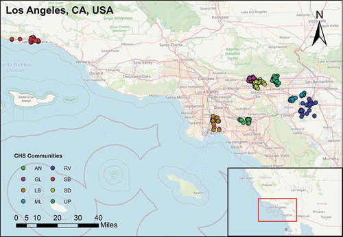
We used data from the CHS ‘Intra-Community Variation 2ʹ (ICV2) sampling campaign (Urman et al. 2014) which was conducted in Anaheim (AN), Glendora (GL), Long Beach (LB), Mira Loma (ML), Riverside (RV), San Dimas (SD), Santa Barbara (SB) and Upland (UP) (Figure 1). These communities range from coastal areas impacted by marine vessel emissions and marine aerosols (SB and LB), to further inland regions impacted by traffic, freight, dairy farming and secondary aerosol formation (AN, UP, GL, SD, ML and RV).

Figure 1. Map of CHS southern California communities participating in the ICV2 sampling campaign (AN = Anaheim, GL = Glendora, LB = Long Beach, ML = Mira Loma, RV = Riverside, SB = Santa Barbara, SD = San Dimas, UP = Upland)

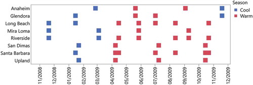
Sampling protocols and quality assurance procedures were described in detail in Fruin et al. (2014) and are summarized here. Month-long chemistry samples were obtained from two consecutive 2-week integrated samples between November 2008 and December 2009 in cool (Oct–Mar) and warm (Apr–Sep) seasons using a rotating deployment schedule (Figure 2) at up to 46 locations per community (Supplement ), with the exception of SB where local wildfire events resulted in a single round of two-week integrated samples. Sampling locations monitored included CHS participants’ residences, schools and central site stations to capture local, neighborhood and regional scale variation in air pollution, respectively. Additional sampling was conducted at the central sites to ensure more complete temporal coverage. Selection of residence locations within communities was based on maximizing the expected variability in traffic source impacts based on earlier modeling (Franklin et al. 2012) and line source dispersion models (Benson 1992).

Figure 2. Timeline of ICV2 rotating sampling schedule per community colored by cool and warm season

Two modified Harvard Cascade Impactors (Lee et al. 2006) with 0.2 µm, 0.5 µm, 2.5 µm and 10 µm cut-points were used to collect two-week integrated PM_0.2, PM_0.2–2.5 (defined as the sum of PM_0.2–0.5 and PM_0.5–2.5) and PM_2.5–10 samples at a flow rate of 5 liters per minute (lpm). Polyurethane foam (PUF) (Kavouras and Koutrakis 2001) was used as the impaction substrate in all stages except for the final 0.2 µm stage, where 37-mm Teflon or quartz filters were used. In addition, a Harvard Personal Environmental Monitor (H-PEM) was used to collect PM_2.5 on pre-baked quartz filters at 1.8 lpm (Supplement Figure S1). Both the PUF substrates and Teflon filters were specially pre-cleaned to remove inorganic and organic contaminants that might compromise quantification at the low levels needed for this study.

Chemical analyses

PM_2.5–10 (coarse), PM_0.2–2.5 (accumulation mode) and PM_0.2 (quasi-ultrafine) mass were determined from stage 2 PUFs, stage 3 + 4 PUFs and stage 5 Teflon filters, respectively, using reference gravimetric methods. A nylon backup filter was placed behind the Teflon filter in stage 5 to capture volatile nitrate losses, and fine and quasi-ultrafine masses were corrected accordingly. To obtain PM_2.5 (fine) mass and composition, PM_0.2 and PM_0.2–2.5 were summed for all chemical analyses. Similarly, PM₁₀ mass was calculated as the sum of PM_2.5–10 and PM_2.5. For consistency with the literature and ease of presentation, PM_2.5–10 will subsequently be referred to as the coarse size fraction, PM_2.5 as the fine and PM_0.2 as the quasi-ultrafine fraction, respectively.

The concentrations of 48 elements (both total and water-soluble) in each size fraction were determined by magnetic-sector inductively coupled plasma mass-spectroscopy (SF-ICP-MS; Thermo-Fisher Element 2) in the Trace Element Cleanroom Facility at the Wisconsin State Laboratory of Hygiene (WSLH) (Clements et al. 2014; Daher et al. 2013; Hays et al. 2011; Okuda, Schauer, and Shafer 2014). For the total analyses, PM was completely solubilized with a mixture of ultra-pure nitric, hydrochloric and hydrofluoric acids using an automated microwave-aided digestion system (Milestone Ethos Plus). The reported total uncertainties in the elemental data incorporate the three major sources of uncertainty (SF-ICPMS measurements, method blank subtraction, and digestion recovery). Elemental and organic carbon concentrations (EC and OC, respectively) in the quasi-ultrafine and fine fraction (not available in coarse) were determined from quartz filters using the thermal-optical transmittance method (TOT NIOSH method 5040). Quartz filters were also used to determine water-soluble organic carbon (wsOC) concentration in these two size fractions using a GE/Sievers 900 TOC Analyzer. Insoluble OC (isOC) was then calculated as the difference between total OC (from EC/OC measurement) and wsOC. Soluble, major cations (sodium, ammonium and potassium) and anions (chloride, nitrate, phosphate and sulfate) were analyzed following water extraction of Teflon filters by ion chromatography (IC) at secondary sites only, defined as schools and central sites.

A summary of the data available in each size fraction at the individual participant residences, schools and central sites is presented in Supplement Table S2. Due to cost considerations, only samples from the quasi-ultrafine size fraction were analyzed in full, and approximately half of the filters in the fine and coarse size fractions were analyzed (selected evenly across seasons). In all analyses, standard QA/QC procedures were followed, including lab and method blank corrections, 10% duplicate samples and sample spikes.

Geospatial traffic variables

In order to further understand spatial determinants of traffic-related PM sources and inform future spatiotemporal modeling efforts, the following commonly used geospatial metrics of TRAP were utilized. These capture spatial variability in different aspects of the traffic mix, including volume, speed and density, tailpipe and non-tailpipe signals, light and heavy-duty vehicles, and stop-and-go versus free-flowing traffic.

The California Line Source Dispersion (CALINE4) model was used to estimate nitrogen oxides (NO_x) concentrations at sampling locations contributed from local on-road vehicle emissions on freeways/highways and non-freeways/highways (major and minor roads) within 5 km during the 4-week sampling period, hereafter referred to as “fwy/hwy NO_x” and “non-fwy/hwy NO_x,” respectively (Benson 1992, 1989). The advantage of CALINE4 is that it incorporates local traffic volumes, emissions from light and heavy-duty vehicles and meteorology (wind direction and speed) in estimating NO_x concentrations at receptor sites using a deterministic Gaussian plume dispersion model. CALINE4 is well suited for estimating vehicle emissions concentrations downwind of roadways on the local scale (Benson 1992; Franklin et al. 2012) and on-road freeway concentrations (Fruin et al. 2011; Westerdahl et al. 2005; Zhu et al. 2002, 2006).

Traffic density was calculated as distance-decayed Annual Average Daily Traffic volume in both directions from all roads within a 300 m circular buffer using a kernel density function with a 300 m search radius and 10 m grid resolution. Total road length was calculated as the sum of the length of all roads within a 300 m radius buffer. Truck percent was calculated as the fraction of heavy-duty vehicles on the nearest freeway (FCC1 road class).

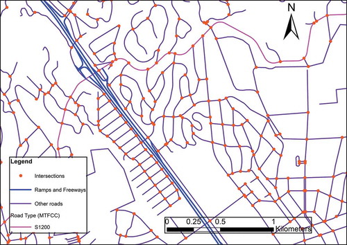
In addition, count of street intersections was calculated by first spatially intersecting 2014 Census Tiger line files for all roads to create intersection points, then removing end of road points and points intersecting limited access highways and ramps in ArcMap 10.5. This resulted in a points layer of intersections along roads (Figure 3), which were then summed within a 250 m or 500 m buffer around each sampling location.

Figure 3. Map illustrating GIS-derived street intersection points

Data analysis

Enrichment ratios

In addition to descriptive statistics and non-parametric correlations, enrichment ratios (ER) (Austin et al. 2013; Landsberger et al. 1992; Parviainen et al. 2020) were calculated for each element to indicate its contributions in the PM_0.2 and the PM₁₀ size fractions relative to PM_2.5, as follows:

(1) $E{R}_{i{j}_{0.2/2.5}}=(X_{i{j}_{0.2}}/P{M}_{j_{0.2}})/\left(X_{i{j}_{2.5}}/P{M}_{j_{2.5}}\right)$(1)

(2) $E{R}_{i{j}_{10/2.5}}=(X_{i{j}_{10}}/P{M}_{j_{10}})/\left(X_{i{j}_{2.5}}/P{M}_{j_{2.5}}\right)$(2)

Where X_ij is the concentration of species i in sample j. Median ER’s were then calculated for all species across all samples and plotted. These ratios reveal information about predominant emission or formation processes, where ratios approaching one indicate elements that are equally enriched in PM_2.5. We expect elements related to primary fresh combustion (potentially also secondary formation) to be smaller in size (<1 µm) and more enriched in PM_0.2 relative to PM_2.5 (median ER_0.2/2.5 > 1); while we expect elements related to crustal and mechanical abrasion sources to be larger in size and more enriched in PM₁₀ relative to PM_2.5 (median ER_10/2.5 > 1) (Hidy 2019).

Source apportionment using the EPA positive matrix factorization model

We used the EPA Positive Matrix Factorization (EPA PMF v5.0) (Norris et al. 2014; Paatero and Tapper 1994) model to apportion measured PM_0.2, PM_2.5 and PM_2.5–10 mass concentrations into their major contributing “sources” or “source groups” (Norris et al. 2014; Paatero and Tapper 1994). Methods are briefly described here, and additional details are included in the supplement for reference. The PMF model solves the following equation:

(3) $x_{ij}=\sum _{k=1}^p{g}_{ik}{f}_{kj}+e_{ij}$(3)

where x_ij is the concentration of species j in sample i, g_ik is the mass contribution of factor k to sample i, f_kj is the loading of species j on factor k and e_ij is the residual error for sample i and species j. PMF solves eq. (3)(3) $x_{ij}=\sum _{k=1}^p{g}_{ik}{f}_{kj}+e_{ij}$(3) by minimizing the following object function (Q) iteratively using the Multilinear Engine v2 (ME-2):

(4) $Q=\sum _{i=1}^n\sum _{j=1}^m{\left[\frac{e_{ij}}{u_{ij}}\right]}^2$(4)

where u_ij is the uncertainty of species j in sample i. Therefore, each observation is individually weighted by its uncertainty. Furthermore, elements of the G and F matrix are restricted to being positive (or non-significantly negative).

Two files were prepared to input to EPA PMF v5.0 – a concentrations file and a sample-specific uncertainties file – for each of the three size fractions. Sample-specific analytical uncertainties were provided by WSLH for metals, OC, EC, wsOC and ions. Any missing concentrations (and in turn uncertainties) were replaced by overall species-specific medians in PMF. Uncertainty values of zero were replaced by a low value (10⁻⁶ ng/m³).

Per PMF guidelines, “Strong” and “Weak” species were included in the analysis and “Bad” species were excluded, based on their signal-to-noise ratio (S/N) as follows: “Strong” S/N ≥ 3, “Weak” 1 ≤ S/N < 3 and “Bad” S/N < 1 (Supplement Table S3). Setting species as “Weak” increases their uncertainty by a factor of 3. However, some exceptions were made to exclude species as follows: Lu in PM_0.2 (S/N = 1.1); Se in all three size fractions (high frequency of missing data); and As, W and chloride ion in PM_0.2; Cr in both PM_0.2 and PM_2.5 for undue influence on the solution resulting in factor smearing. Out of all available samples, 6.5% (30 out of 461), 5.7% (15 out of 250) and 1% (3 out of 298) were excluded as outliers from the analysis based on species’ concentrations in PM_0.2, PM_2.5 and PM_2.5–10, respectively.

An additional 10% modeling uncertainty was added to all runs to account for sampling and modeling errors not captured in the analytical uncertainties. Five to nine factors were attempted for all size fractions, and the optimal factor number was chosen based on the solution with the most physically interpretable results and least factor smearing. Solution stability evaluation, rotations, and uncertainty evaluations are described in further detail in the supplement. Factors were identified based on the loading of species in their profiles and knowledge of expected spatial and temporal patterns in their contributions.

Spatial variation and determinants of traffic-related PM sources

Given the complex and often non-linear correlations of traffic-related, tailpipe and non-tailpipe PM sources across size fractions, we further investigated their spatial variation and potential determinants to identify top candidate predictors and inform future exposure modeling efforts. Predicted contributions for traffic-related sources were first averaged for each sampling location to remove the influence of any temporal factors in this spatial analysis.

The MapGAM package (Bai et al. 2019) in R (Team RC 2019) was used to fit generalized additive models (GAMs) of traffic-related PM sources. The utility of these nonparametric GAMs is in their ability to capture non-linear relationships among covariates (or predictors) and to generate smooth prediction surfaces that can reveal more complex relationships than standard linear approaches. In other words, GAMs allow the effect of variables on predicted sources to change or vary at different levels of the predicted source, rather than remain static or fixed. All variables were standardized (mean = 0, standard deviation = 1) to ensure they were on a similar scale since the loess smooth uses a spherical (isotropic) neighborhood when establishing nearest neighbors, and Spearman correlation coefficients were calculated.

Primary models included a bivariate loess smooth term with latitude and longitude to examine spatial variability in these sources (or whether geographic location was a significant predictor of these sources). In secondary analyses, geospatial metrics were used in the bivariate smooth (instead of geographic coordinates) to examine the combined “mixture” effect of two parameters at a time on predicted sources. The optimal span for each model was determined by searching from 0.10 to 0.90 in 0.05 increments. Predictions were generated and mapped across an equally spaced grid over the study domain with black contour lines indicating regions with significantly higher (red) or lower (blue) levels at an alpha = 0.05 level. In sensitivity analyses, Long Beach was excluded to examine its influence on observed patterns since it has some of the highest heavy-duty truck activity in the region, which might overshadow smaller signals from light-duty vehicles.

Finally, a significance threshold of p-value < .0005 for the non-parametric loess term (ANOVA F test) was used as a conservative approach to protect against chance findings due to multiple testing. For brevity, only models with a clear pattern of change in the predicted source along both x and y dimensions (when x and y are two geospatial metrics) and a more stringent p-value < .0001 for the “mixture” effect are reported in the main manuscript; remaining significant models are included in the supplement.

Results

Descriptive statistics of PM and elemental concentrations in the quasi-ultrafine, fine and coarse size fractions are presented in Table 1. Bar plots comparing concentrations of elemental species across size fractions are also provided in Supplement Figure S2.

Table 1. Descriptive statistics of PM and elemental concentrations in the quasi-ultrafine, fine and coarse size fractions

		Quasi-Ultrafine, PM0.2			Fine, PM2.5			Coarse, PM2.5–10
Units: ng/m^3		N	Mean	Std Dev	N	Mean	Std Dev	N	Mean	Std Dev
PM Mass		470	2,389.6	884.6	484	14,599.1	3,890.3	496	12,854.4	4,713.9
Carbon Species
	EC	461	364.7	192.5	470	873.6	483.0
	OC	460	1,069.8	383.1	471	2,784.9	991.1
	Water-soluble OC	460	426.6	136.3	473	975.6	305.8
	Water-insoluble OC	458	641.6	293.0	470	1,798.9	864.6
Ions*
	Ammonium	94	101.9	87.1	93	362.8	182.5	93	89.9	57.7
	Chloride	94	35.3	92.0	93	71.7	105.7	93	540.6	511.1
	Nitrate	93	127.7	249.9	92	781.5	541.8	93	1,803.8	706.1
Elements
	Al	461	1.6	1.8	265	51.9	32.0	298	408.0	328.8
	Ba	461	0.2	0.3	265	5.5	3.9	298	18.1	12.2
	Ca	461	2.1	2.4	265	55.5	33.0	298	383.1	296.2
	Cr	461	0.0	0.1	265	0.3	0.3	298	1.1	0.7
	Cu	461	0.2	0.3	265	3.8	2.7	298	10.5	7.4
	Fe	461	3.7	3.8	265	85.8	56.4	298	430.8	319.2
	K	461	7.4	7.2	265	46.1	20.5	298	172.7	133.4
	Mg	461	0.7	1.0	265	36.4	14.5	298	190.1	124.9
	Mn	461	0.1	0.2	265	1.6	1.2	298	6.8	5.2
	Na	461	3.9	3.8	265	194.1	116.8	298	821.5	699.4
	P	461	0.5	0.5	265	4.7	3.7	298	20.4	23.6
	Pb	461	0.5	0.5	265	1.5	0.9	298	1.2	0.8
	S	461	54.0	37.6	265	328.3	137.6	298	167.9	107.3
	Sb	461	0.2	0.1	265	1.0	0.7	298	1.7	1.3
	Sr	461	0.1	0.1	265	0.8	0.4	298	3.6	2.3
	Ti	461	0.3	0.6	265	5.6	3.6	298	34.5	26.0
	V	461	0.5	0.5	265	1.7	1.0	298	1.0	0.7
	Zn	461	1.3	2.8	265	6.4	7.4	298	9.5	8.2
Units: pg/m^3
	Ag	461	4.0	5.0	265	13.1	9.7	298	14.7	10.2
	As	461	63.1	62.0	265	173.2	88.3	298	132.6	91.5
	B	461	674.4	405.1	265	1,337.1	612.4	298	539.1	446.6
	Cd	461	14.1	24.8	265	52.9	45.5	298	22.0	14.6
	Ce	461	6.5	7.2	265	115.3	65.6	298	512.3	348.8
	Co	461	4.2	7.9	265	38.7	35.7	298	163.9	123.0
	Cs	461	0.5	0.6	265	5.7	3.1	298	29.1	22.0
	Dy	461	0.1	0.1	265	2.8	1.7	298	22.0	16.9
	Ho	461	0.0	0.0	265	0.6	0.3	298	4.4	3.4
	La	461	4.6	4.8	265	115.6	77.8	298	314.3	215.1
	Li	461	9.0	17.2	265	110.1	132.6	298	295.5	239.0
	Lu	461	0.0	0.0	265	0.3	0.2	298	1.9	1.4
	Mo	461	70.8	126.4	265	275.8	268.6	298	442.8	312.9
	Nb	461	0.8	2.3	265	14.7	8.0	298	84.9	59.9
	Nd	461	0.8	0.8	265	23.2	12.6	298	159.3	113.9
	Ni	461	148.9	203.9	265	683.1	488.7	298	703.9	480.8
	Pd	461	0.4	0.5	265	6.0	3.5	298	28.7	17.8
	Pr	461	0.3	0.3	265	7.3	3.9	298	44.7	31.0
	Pt	461	0.2	0.6	265	2.9	5.9	298	5.6	8.6
	Rb	461	9.4	8.8	265	96.0	55.0	298	592.0	490.0
	Rh	461	0.1	0.1	265	0.7	0.5	298	1.8	1.2
	Sc	461	0.4	0.7	265	9.3	5.9	298	72.1	56.7
	Se	45	80.0	29.2	47	235.9	70.7	54	84.8	50.3
	Sm	461	0.1	0.1	265	4.6	2.5	298	29.7	21.8
	Th	461	0.4	0.9	265	8.6	4.8	298	59.8	43.0
	Tl	461	1.7	2.0	265	5.2	3.4	298	4.5	3.5
	U	462	0.2	0.2	266	3.5	1.9	299	23.0	16.3
	W	461	17.6	24.6	265	61.9	54.2	298	106.1	76.0
	Y	461	0.5	1.2	265	18.3	11.3	298	141.2	98.1
	Yb	461	0.0	0.1	265	1.7	1.1	298	12.7	9.7

Notes. *Only measured ions concentrations collected at schools and central sites are summarized. Values at residences were imputed from community- and sampling period-specific measurements.

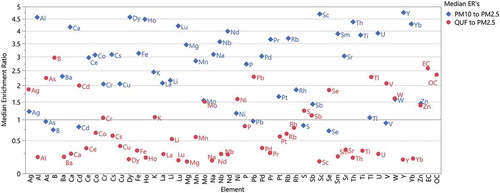
On average, EC constituted 15.8% and 6.3% of ultrafine and fine PM mass, respectively, while OC constituted 46.9% and 19.9% of the ultrafine and fine PM mass, respectively. The soil-related elements Y, Sc, Dy, Al, and Ho had the highest median enrichment ratios in PM₁₀ compared to PM_2.5; whereas, B, EC, and OC – species related to vehicular traffic tailpipe emissions – had the highest median enrichment ratios in the PM_0.2 compared to the PM_2.5 (Figure 4). The elements As, Pb, Tl, V and Cd were also some of the most enriched in PM_0.2 compared to PM_2.5 which reflects the relatively high volatility of these elements. The distribution of enrichment ratios for all species is presented in Supplement Table S4.

Figure 4. Median enrichment ratios in the PM₁₀ (blue diamonds) and PM_0.2 quasi-ultrafine (red circles) size fractions relative to PM_2.5.

Source apportionment

PMF solutions and model performance

A total of six, seven and five factors were selected as the optimal, physically interpretable solutions in PMF. These factors together explained 63%, 86% and 88% of the variability in PM_0.2, PM_2.5 and PM_2.5–10 mass, respectively (Table 2).

Table 2. Summary of PMF model performance in each size fraction (R² and intercept from base model, mean predicted mass from final rotated solutions)

		Measured		Predicted*		Intercept (% Unexplained Mass)
Size Fraction	N Factors	Mean (ng/m^3)	N Obs	Mean (ng/m^3)	R^2	Mean (ng/m^3)	%
PM0.2	6	2,347.6	431	2,167.7	0.63	593.9	25.3
PM2.5	7	14,018.5	250	13,868.5	0.86	679.5	4.8
PM2.5–10	5	11,713.8	295	11,660.7	0.88	33.7	0.3

R²’s for individual species and tests of normality for the residuals are presented in Supplement Table S5. In general, R²’s were lowest in the quasi-ultrafine size fraction, likely due to the lower concentrations and greater challenges in measuring mass concentrations accurately in this size fraction, with the exception of a few species (V, S, Zn, Rh, La, etc.) with the highest R² in the quasi-ultrafine fraction.

In initial runs, including Cr in the model resulted in a single Cr factor with highest contributions in SB and LB, both coastal communities, with remaining uninterpretable, smeared factors. While the Cr signal could be related to chromium plating, Cr was ultimately set to “Bad” and excluded from the PM_0.2 and PM_2.5 model solutions to obtain physically interpretable solutions. Similarly, keeping As and W in the PM_0.2 model resulted in them separating into a single factor with zero (negligible) estimated mass.

Predicted source profiles and contributions

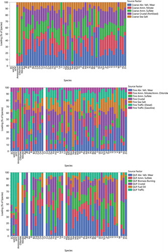
PMF-resolved factors were identified based on their loading profiles (Figure 5, and Supplement Figure S3 for individual plots of factor profiles) and spatial and temporal patterns in their source contributions (Supplement Figures S4.A and S4.B, respectively).

Figure 5. Source profiles (in % of species) in the quasi-ultrafine, fine and coarse PM size fractions

Mean predicted source contributions by size fraction overall and by community are shown in Figures 6 and 7, respectively.

Figure 6. Percent contribution of A) all PMF-predicted sources to total PM mass and B) tailpipe and non-tailpipe sources to total traffic-related PM mass in each size fraction (averaged across all communities)

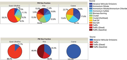
Figure 7. Percent contribution of PMF-predicted sources to total PM mass in each size fraction by community

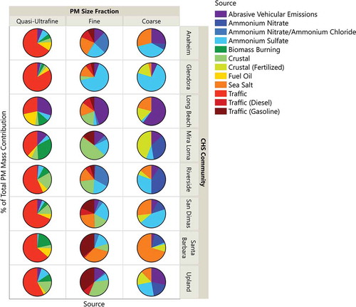
The study communities (as shown in Figure 1) range from coastal areas heavily impacted by primary marine vessel, port and traffic emissions with cooler temperatures and predominantly Westerly winds, to communities further inland with more significant impacts of secondary aerosol formation as a result of higher temperatures and conditions favoring photochemical reactions (Daher et al. 2013). In general, some categories of sources were identified in all three size fractions – such as abrasive vehicular emissions (AVE) and secondary inorganic PM (ammonium nitrates and ammonium sulfates); whereas, others were only distinguishable in a single size fraction (e.g., biomass burning).

Quasi-ultrafine PM sources

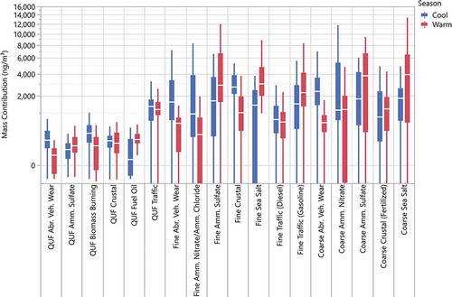
The six sources resolved in the quasi-ultrafine size fraction consisted of the following: “Traffic” constituted 58.2% of the PM_0.2 mass and had high loadings of EC, wsOC, isOC and B. Boron is a known gasoline fuel additive (Shah, Glavatskih, and Antzutkin 2013). “Fuel Oil” had the highest loadings of Ni and V and contributed 8.3% of the PM_0.2 mass, with the highest contributions in the port community of LB. “Crustal” had high loadings of Al, Ca, Yb and Ho and contributed 9.2% of the PM_0.2 mass. “Biomass Burning” was marked with high loading of K, Rb and wsOC and contributed 11.1% of the PM_0.2 mass with higher contributions in the cool season (Figure 8). “Abrasive Vehicular Emissions” (AVE) contributed 7.7% of the PM_0.2 mass and was marked by high loadings of tire, brake and catalyst wear markers Ba, Cu, Mo, Sb, Zn, Pt and Pd. It is important to note that this factor is named “AVE” given the high loadings of brake and tire abrasion markers; however, it also contains the platinum group metals Pt, Pd and Rh which are typically released from the attrition of catalysts through the tailpipe. This distinction applies to all subsequent references to “AVE” sources. “Ammonium Sulfates” had high loading of lanthanum (La), a marker of petroleum refineries emissions (Kulkarni, Chellam, and Fraser 2007), in addition to ammonium ion and sulfur (S) and contributed 5.5% to the PM_0.2 mass. Contributions were higher in the warm season (Figure 8).

Figure 8. Distribution of PMF-predicted source contributions by season. The horizontal white line inside the boxplots indicates the median, the bottom and top edges of the boxes indicate the 1st and 3rd quartile, respectively, and the bottom and top whiskers extend to the outermost data points that fall within distances defined using the interquartile range (IQR) as 1st quartile – (1.5*IQR) and 3rd quartile + (1.5*IQR), respectively

Fine PM sources

In the PM_2.5 size fraction, seven source factors were resolved as follows: “Ammonium Sulfates” with high loadings of La and S, possibly related to secondary formation from petroleum refineries and industrial emissions (Kulkarni, Chellam, and Fraser 2007). It contributed 22.8% of the total PM_2.5 mass. Two tailpipe traffic sources were identified in PM_2.5 – “Traffic (gasoline)” with loadings of wsOC, isOC and B (15% of the mass) and “Traffic (diesel)” with loadings of EC and barium (Ba) (5.9% of the mass). “Traffic (gasoline)” was elevated in most communities with major freeways (SB, ML, SD, UP) while “Traffic (diesel)” was elevated in communities with truck activity (LB, AN, SD, GL). “Sea Salt” also contributed 15.9% of PM_2.5 mass, with loadings of Na, Cl and Mg, and highest contributions in the coastal community of SB. “Abrasive Vehicular Emissions” (AVE) was also resolved, with an 11.4% contribution to mass and high loadings of Ag, Mo, Zn, Ni, V, Pt and Rh. This factor was highest in communities with significant truck and freight activity (LB, ML, AN), and the presence of Ni and V here suggests a certain degree of collinearity with fuel oil sources originating from source areas in close proximity (i.e., the ports) (Habre, Coull, and Koutrakis 2011). “Crustal” (19% of PM_2.5 mass) was also resolved with Al, Dy and Fe – elements related to soil – and highest contributions in the inland, arid community of ML with agricultural and dairy production. Finally, a factor related to secondary inorganic PM formation was identified with high loadings of ammonium, nitrate and chloride (“Ammonium Nitrate/Ammonium Chloride”). It contributed ~10% of PM_2.5 mass and had highest contributions in the cool season in RV (Figure 8). This is a result of ammonia (NH₃) reactions with nitric and hydrochloric acid, which is shown to favor formation of ammonium nitrate and ammonium chloride especially in cold conditions (Kelly et al. 2013; Wang et al. 2015).

Coarse PM sources

Finally, in the PM_2.5–10 size fraction, the following five sources were resolved: “Crustal (fertilized soil)” with Al, Ca, Dy, K, Rb and P loadings contributing 15.6% of the mass with highest concentrations inland in ML. “Ammonium Nitrate” (17.6% of mass) had highest contributions inland as well, downwind of the dairy farms producing ammonia in ML and RV and was somewhat higher in the cool season (Figure 8). “Abrasive Vehicular Emissions” (AVE) with Cu, Ba, Mo, Sb, Rh, and Pt contributed 18% of the PM_2.5–10 mass and was highest in LB, AN and ML. The presence of some crustal elements (Al, Ca) here also suggests some mixing with road dust. “Sea Salt” with Na, chloride and S (22.7% of mass) was highest in SB and LB. Finally, “Ammonium Sulfate” contributing 26.1% of the mass was higher in the warm season, with ammonium, nitrate and S (Figure 8).

Detailed results examining the variability in the PMF solution by bootstrapping, displacement analyses or Fpeak rotation are presented in Supplement Table S6. Briefly, PM_0.2 sources were minimally displaced in these evaluations; whereas, diesel traffic exhibited some swapping (13%) with AVE, and secondary ammonium nitrate/chloride with crustal (10%) in PM_2.5 Fpeak bootstraps. Finally, the crustal source mapped to AVE in 18% of Fpeak bootstraps in PM_2.5–10 implying greater difficulty in distinguishing these two sources in the coarse fraction.

Overall, tailpipe and non-tailpipe traffic-related sources together contributed around 66%, 32% and 18% of PM_0.2, PM_2.5 and PM_2.5–10 mass, respectively; with non-tailpipe AVE sources contributing around 8%, 11% and 18% of PM mass, respectively. Tailpipe traffic sources were resolved in PM_0.2 and PM_2.5 only, as one source in PM_0.2 and as two gasoline and diesel sources with differentiated source profiles in PM_2.5. Non-tailpipe traffic sources were resolved in all three size fractions with similar chemical signatures, although with some collinearity with diesel traffic (in PM_2.5) and crustal (in PM_2.5–10).

Spearman correlation coefficients between the resolved PM sources are presented in Supplement Table S7. Fuel oil (PM_0.2) was correlated with sea salt (PM_2.5) likely due to the proximity of their sources (ports and ocean). Sea salt in PM_2.5 and PM_2.5–10 had a 0.67 correlation. Tailpipe combustion-related traffic sources in PM_0.2 and PM_2.5 were not highly correlated suggesting they are potentially capturing different components of the traffic mixture. Whereas, non-tailpipe AVE sources exhibited high correlations with each other across all three size fractions (>0.79).

Location as a predictor of tailpipe and non-tailpipe traffic sources

Predicted surfaces from GAM models using geographic location as a bivariate smooth to predict standardized levels of traffic-related sources are shown in Figure 9A (all communities) and Figure 9B (excluding Long Beach).

Figure 9A. Predicted surfaces of traffic-related sources from GAM models on standardized scale. Contour lines delineate areas (locations) of statistically significant higher (red) or lower (blue) concentrations. Vertical lines in color scale indicate median values

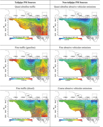
Figure 9B. Predicted surfaces of traffic-related sources from GAM models on standardized scale, excluding Long Beach from the analysis. Contour lines delineate areas (locations) of statistically significant higher (red) or lower (blue) concentrations. Vertical lines in color scale indicate median values

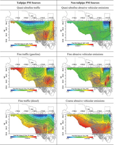
Tailpipe traffic in PM_0.2 was generally elevated across the basin, while gasoline traffic in PM_2.5 showed elevated levels in areas close to SB, GL, SD and UP – all communities with important freeway and highway traffic activity. In contrast, diesel traffic in PM_2.5 was elevated around LB and further inland toward ML along the truck and freight transport corridor. Non-tailpipe AVE sources exhibited generally similar patterns in space across all size fractions and were highest in the core, coastal area of the basin with the most primary emissions. However, when LB was excluded from the analysis, spatial patterns for tailpipe TRAP sources generally remained similar but increased in range (greater predicted levels) in an expected direction (greater where freeways/highways are located, and greater around LB for diesel traffic in PM_2.5). Spatial patterns of non-tailpipe AVE sources changed dramatically with higher predicted levels further inland in PM_0.2, in the urban core for PM_2.5 and across the entire modeling domain for PM_2.5–10. The maximum predicted range of AVE also decreased in PM_2.5 and PM_2.5–10.

Geospatial metrics as potential predictors of traffic-related PM sources

The distribution of geospatial metrics is presented in Supplement Table S7. Spearman correlations between the traffic-related sources (averaged in space and standardized) and geospatial metrics are shown in Supplement Tables S8.A (all communities) and S8.B (excluding Long Beach).

Tailpipe traffic in PM_0.2 was most correlated with intersections within 500 m and 250 m (r = 0.31 and r = 0.29, respectively) followed by total road length (300 m) (r = 0.22). These correlations became stronger once LB was excluded (r up to 0.42 with intersections (500 m)). It was also moderately inversely correlated with gasoline traffic in PM_2.5 (r = −0.18 overall, r = −0.34 excluding LB), but positively correlated with diesel traffic in PM_2.5 (r = 0.12 overall, r = 0.27 excluding LB). In general, geospatial metrics had low negative correlations with the gasoline traffic source but were positively correlated with the diesel traffic source in PM_2.5, with fwy/hwy NO_x (r = 0.55), non-fwy/hwy NO_x (r = 0.46) and traffic density (300 m) (r = 0.43) showing the highest correlations (even when LB was excluded).

In addition, non-tailpipe AVE in PM_2.5–10 and PM_0.2 were most correlated with fwy/hwy NO_x (r = 0.67 and r = 0.50, respectively, similarly once LB was excluded). Whereas, AVE in PM_2.5 was most strongly correlated with truck percent on nearest FCC1 (freeway) even once LB was excluded. Non-fwy/hwy NO_x was also more highly correlated with AVE in PM_2.5–10 (r = 0.62) and PM_2.5 (r = 0.32) compared to PM_0.2 (r = 0.26).

Bivariate relationships between geospatial metrics and traffic-related PM sources

Supplement Figure 10 shows predicted standardized values of select tailpipe (Supplement Figure 10A) and non-tailpipe (Supplement Figure 10B), traffic-related PM sources as a function of two geospatial metrics (mixtures) where p-value < .0001. All remaining GAM models with p-value < .0005 for the bivariate loess smooth term are presented in Supplement Figures S5.A (all communities) and S5.B (excluding Long Beach) and Supplement Table S10.

Simultaneous increases in fwy/hwy NO_x and truck percent, or in intersections (250 m) and truck percent, were associated with higher predicted levels of tailpipe diesel traffic in PM_2.5. A similar pattern was observed with non-fwy/hwy NO_x and truck percent. The prediction range for models including truck percent dropped once LB was excluded, and patterns remained similar except the relationship between truck percent and non-fwy/hwy NO_x on diesel traffic (PM_2.5) became less apparent.

As for tailpipe traffic in PM_0.2, the effect of a simultaneous increase in non-fwy/hwy NO_x and intersections (250 m) became apparent only once LB was excluded (Supplement Figure S5.B).

Similarly, for non-tailpipe AVE sources (Supplement Figure 10B), simultaneous increases in fwy/hwy NO_x and truck percent, or in non-fwy/hwy NO_x and intersections (500 m) were associated with higher AVE in PM_2.5–10 and PM_2.5. The interaction between truck percent and non-fwy/hwy NO_x was most apparent in PM_0.2. Excluding LB resulted in attenuated but still significant influence of truck percent in general, and greater influence of non-fwy/hwy NO_x in all size fractions, especially as intersections (250 m and 500 m) increased in PM_0.2.

Discussion

In this analysis, we were able to distinguish and quantify the contribution of tailpipe and non-tailpipe traffic-related sources among other major primary and secondary sources of PM in southern CA, in the quasi-ultrafine (PM_0.2), fine (PM_2.5) and coarse (PM_2.5–10) size fractions. We found that overall traffic-related sources contributed ~66%, 32% and 18% of PM_0.2, PM_2.5 and PM_2.5–10 mass, respectively, with the PM_2.5–10 traffic contribution consisting entirely of non-tailpipe AVE. We resolved distinct gasoline versus diesel tailpipe traffic profiles in PM_2.5, while non-tailpipe AVE sources had similar chemical signatures in all three size fractions and exhibited some collinearity with diesel traffic in PM_2.5 and crustal in PM_2.5–10.

We also found that the spatial distribution of tailpipe traffic sources in PM_0.2 and PM_2.5 was similar. Higher predicted gasoline traffic emissions (PM_2.5) were observed in areas with major freeways and highways, and higher predicted diesel traffic emissions (PM_2.5) were more localized around the ports and cargo movement activities in LB and further inland. Long Beach, with its extensive heavy-duty truck traffic activity, had a strong influence on observed spatial patterns of non-tailpipe AVE in all size fractions, pulling the highest predicted AVE levels toward the port area and urban core. Once excluded, the impact of inland freeways and highways and light-duty vehicular traffic areas became more apparent on AVE in PM_0.2 and PM_2.5, while predicted AVE in PM_2.5–10 was elevated across the entire basin (although the prediction range decreased).

Similarly, using bivariate GAMs to model non-linear relationships between commonly used geospatial metrics and traffic-related sources, several mixture effects were revealed that would not have otherwise been apparent using standard linear correlations or approaches. Below we discuss our findings in more detail, starting with our general source apportionment modeling results followed by a more focused discussion of tailpipe and non-tailpipe traffic sources and their determinants.

Overall source apportionment findings

Our PMF modeling results are in agreement with previously published literature from southern CA (Arhami et al. 2009; Cheung et al. 2011a, 2011b; Christoforou et al. 2000; Daher et al. 2013; Hasheminassab et al. 2014a, 2014b, 2013). We found traffic to be the largest contributor to PM_0.2 mass (Hasheminassab et al. 2013), while secondary aerosol (ammonium nitrates and ammonium sulfates) contributed the most to PM_2.5 mass (Hasheminassab et al. 2014a, 2014b), followed by primary gasoline and diesel vehicular emissions (Hasheminassab et al. 2014a). However, while other studies found mineral and crustal material contributed the most to PM_2.5–10 followed by abrasive vehicular wear, in our work, secondary aerosol (~44%) contributed slightly more than the crustal (fertilized soil) and AVE sources combined (~33%) (Cheung et al. 2011a, 2011b; Pakbin et al. 2011). We also resolved fuel oil in PM_0.2 (which has been extensively documented as a result of heavy fuel oil use in marine vessels and port operations in Long Beach (Arhami et al. 2009; Minguillon et al. 2008), biomass burning (PM_0.2) (Hasheminassab et al. 2014b; Minguillon et al. 2008), crustal (in all size fractions, distinguished by an additional fertilizer signal in PM_2.5–10 likely due to agricultural activity in Mira Loma) and sea salt (Hasheminassab et al. 2014b; Sowlat, Hasheminassab, and Sioutas 2016).

As for secondary inorganic aerosols, ammonium sulfate was resolved in all size fractions with high loadings of La in PM_0.2 and PM_2.5, suggesting emissions from petroleum refineries are contributing to secondary PM (Du and Turner 2015; Kulkarni, Chellam, and Fraser 2007). Ammonium sulfate is formed as a result of a series of reactions between sulfur dioxide and ammonia (ammonium) under warmer temperature conditions, which also favor photochemical ozone formation (Christoforou et al. 2000; Hasheminassab et al. 2014b; Schiferl, Heald, and Nowak et al. 2014). Ammonium nitrates were resolved in PM_2.5 (with ammonium chloride) and PM_2.5–10. Ammonium nitrate forms as a result of ammonia and nitric acid reactions under cool temperatures which shift the equilibrium into the particle phase. Ammonia is emitted from upwind agricultural and dairy production in Mira Loma, while nitric acid is formed as a result of the oxidation of nitric oxides emitted from primary fuel combustion sources (Wang et al. 2015; Ying and Kleeman 2006; Ying, Lu, and Kleeman 2009). Coarse nonvolatile sodium nitrate is also formed by heterogeneous replacement of chloride by nitrate in coarse sea-salt particles (Gard, Kleeman, and Gross et al. 1998) which may explain the large percentage of secondary aerosol in PM_2.5–10. Ammonium chloride can also form under similar conditions as a result of hydrochloric acid reactions with ammonia (Hayes, Ortega, and Cubison et al. 2013; Kelly et al. 2013; Schiferl, Heald, and Nowak et al. 2014; Wang et al. 2015).

Tailpipe traffic sources

Gasoline and diesel tailpipe traffic was resolved as one combined source in PM_0.2 and as two distinct sources in PM_2.5. Boron, a gasoline fuel additive (Shah, Glavatskih, and Antzutkin 2013, 2012), loaded on both PM_0.2 traffic and PM_2.5 gasoline traffic sources; while EC, a marker of diesel combustion, loaded on both PM_0.2 traffic and PM_2.5 diesel traffic sources (Christoforou et al. 2000; Lough and Schauer 2007). Overall, despite referring to these sources as tailpipe traffic (from on-road vehicles), it is possible for them to have captured some of the contributions of gasoline or diesel-operated off-road mobile vehicular sources impacting these receptor locations if they share similar chemical signatures.

Of these sources, PM_2.5 diesel traffic displayed the highest correlations with examined geospatial metrics, followed by PM_0.2 traffic which correlated weakly with intersections suggesting it could be capturing tailpipe emissions from acceleration in stop-and-go traffic. However, a significant relationship between non-fwy/hwy NO_x and intersections (250 m) on PM_0.2 traffic was revealed once LB excluded (Supplement Figure S5.B). This smaller spatial scale of influence was masked using standard linear correlations. Similarly, for PM_2.5 diesel traffic, bivariate GAMs revealed a joint effect of fwy/hwy NO_x with truck percent, and fwy/hwy NO_x with intersections (250 m) at a smaller spatial scale. This is consistent with (Karner, Eisinger, and Niemeier 2010) findings showing EC (marker of PM_2.5 diesel traffic) decays from the edge of the road to background within very short spatial scales (~130 m).

Non-tailpipe traffic sources

To our knowledge, this is one of very few studies finding non-negligible contributions of AVE across the entire quasi-ultrafine to coarse PM size distribution (minimum of ~8% in PM_0.2 and up to 18% in PM_2.5–10 on average), with important differences across communities. In Long Beach, the average predicted contribution of AVE reached up to 30%, 45% and 59% of PM_0.2, PM_2.5 and PM_2.5–10 mass, respectively, likely due to its concentrated heavy-duty vehicle (truck) activity. Earlier work has mainly focused on AVE signals in PM₁₀ or PM_2.5, with much fewer studies reporting brake, tire and catalyst wear signals in PM_0.2 or smaller. Kuwayama, Ruehl, and Kleeman (2013) found brake wear and road dust source in PM_0.1 marked by Fe, Cu, Zn and Pb in Sacramento, CA. Hays et al. (2011) found elevated catalyst (Pt, Rh, Pd) in the 1–2 µm aerodynamic diameter range and brake and tire wear (Cu and Sb) markers in the ≥1–4 µm range in a near-highway study with predominantly light-duty gasoline vehicles. Several studies have documented the presence of platinum group metals from catalyst attrition in airborne and settled traffic-related PM and road dust (Ely et al. 2001; Wiseman and Zereini 2009; Zereini, Alsenz, and Wiseman et al. 2012; Zereini, Wiseman, and Püttmann 2007). Laboratory dynamometer testing of a variety of modern brake materials showed that the PM₁₀ mass from brake wear consisted of 27%, 35% and 38% coarse (PM_10–2.5), fine (PM_2.5–0.1) and ultrafine particles, respectively (Garg et al. 2000). Increasingly, studies are showing non-negligible contributions of ultrafine brake wear particles to total PM₁₀ (Nosko and Olofsson 2017; Thorpe and Harrison 2008), with higher temperature increasing emissions in the ultrafine range (Grigoratos and Martini 2015; Shin et al. 2019). These findings underscore potentially important implications for near-roadway exposures as tailpipe emissions decrease because of clean technologies while non-tailpipe emissions increase in relative importance, especially in the smallest PM_0.2 size fraction.

In terms of potential geospatial predictors, AVE in PM_0.2 and PM_2.5–10 were most correlated with fwy/hwy NO_x, while AVE in PM_2.5 was most correlated with truck percent. Non-fwy/hwy NO_x was also highly correlated with AVE in PM_2.5–10 and to a lesser extent AVE in PM_2.5. However, in bivariate GAMs, truck percent was significantly related to AVE in all size fractions as NO_x increased. These relationships were heavily driven by Long Beach data. This suggests that the impact of light-duty vehicles on AVE was masked when LB data were included with its predominantly heavy-duty vehicle impact. Similarly, the impact of smaller roads with light-duty vehicles (non-fwy/hwy NO_x) and stop-and-go traffic (intersections (500 m)) on AVE in PM_0.2 was revealed once LB was excluded.

Overall, LB was much more influential in non-tailpipe traffic analyses compared to tailpipe, and CALINE4 line source dispersion estimates, trucks on nearest freeways and intersections strongly influenced predicted AVE levels in interrelated ways, and within small spatial scales. These results are in line with recent work in Boston that found strong spatial gradients away from major roadways for markers of AVE (e.g., Ba, Zn, Cu, Fe) in PM_2.5 and PM_2.5–10 size fractions (Koutrakis et al. 2018). Oakes et al. (2016) also showed brake wear metals Ba and Cu were most enriched in PM_2.5 and PM₁₀ within 100 m of a major interstate in Detroit, Michigan.

Trends in traffic emissions as a result of mobile source regulations

Our results show important contributions of AVE to traffic emissions in all three size fractions, and especially in areas with significant heavy-duty truck activity and ports. Our data were collected in 2008–9 as part of the CHS with the goal of modeling traffic-related PM exposures of participants and retrospectively assessing their impacts on health. However, since 2009, several federal and state mobile source control regulations have come into play in southern California for both on-road and off-road vehicles, engines and equipment (Lurmann, Avol, and Gilliland 2015).

Among those affecting tailpipe emissions, the California Air Resources Board (CARB) Truck and Bus Rule requires all heavy-duty diesel vehicles to reduce engine emissions of PM, NO_x and air toxics (Board 2018). The federal U.S. Environmental Protection Agency’s (EPA) Tier 3 Motor Vehicle Emission and Fuel Standards program required reductions in tailpipe and evaporative emissions from most light- and medium-duty and some heavy-duty vehicles and lowered the sulfur content of gasoline fuel starting in 2017 (Agency 2014). Overall, these regulations have led to reductions in on-road, tailpipe PM emissions from light, medium and heavy-duty vehicles over time. For example, Bishop (2019) measured on-road tailpipe emissions in Lynwood, CA in 1989, 1999 and 2018 and reported reductions of up to a factor of 20 for carbon monoxide and up to a factor of 25 for hydrocarbons in tailpipe emissions in 2018 compared to the early 1990s.

As for non-tailpipe emissions, some of the major regulations include the Federal Motor Vehicle Safety Standard (FMVSS 121) which required a reduction in stopping distance for heavy-duty trucks starting in 2011 (Caltrans Division or Research Innovation and System Information DoEA 2017). As a result, new materials with better stopping power such as semi-metallic brake linings are increasingly being used, and these release more airborne PM than traditional ceramic or metallic brakes (Caltrans Division or Research Innovation and System Information DoEA 2017). California legislation SB 346 also regulated hazardous material content in brake pads starting in 2014, with the goal of reducing copper weight content to 5% by 2021 and 0.5% by 2025. This is expected to influence the chemical composition and potentially size distribution (PM₁₀ to PM_2.5 ratios) of brake wear PM emissions (Caltrans Division or Research Innovation and System Information DoEA 2017). Finally, regenerative braking systems in electric and hybrid light- and heavy-duty vehicles are expected to significantly lower brake wear emissions especially at low speeds (<30 mph) (Caltrans Division or Research Innovation and System Information DoEA 2017).

In terms of tire wear emissions, with the push for more fuel economy (for example, Corporate Average Fuel Economy (CAFE) standards), lower rolling resistance tires are increasingly used, and these are thought to have higher tire wear emission rates (Caltrans Division or Research Innovation and System Information DoEA 2017). Other trends include increased use of larger brake pads and larger tire sizes with potentially unclear implications. Taken together, it is difficult to quantify the net impact of these regulations and trends on overall non-tailpipe AVE emissions. However, tailpipe emission reductions are likely resulting in a higher relative contribution of non-tailpipe sources to total traffic-related PM emissions over time (Thorpe and Harrison 2008).

Implications for exposure modeling and health analyses

Our work demonstrates the challenges involved in isolating and modeling the independent impacts of tailpipe and non-tailpipe traffic on observed PM concentrations. It also illustrates the extent to which mixture modeling approaches (e.g., bivariate GAMs) can uncover more complex and non-linear relationships among geospatial metrics in terms of how they might jointly influence concentrations of traffic-related PM.

Despite our robust PMF modeling results, collinearities in source profiles (e.g., similar physiochemical fingerprints) or contributions (e.g., similar source areas, or emissions, dispersion and removal patterns) (Habre, Coull, and Koutrakis 2011; Tian et al. 2014) can still complicate source apportionment. For example, like in other studies (Thorpe and Harrison 2008), we had difficulty discerning AVE from resuspended road dust in the PM_2.5–10. We also had difficulty disentangling fuel oil burning (marked by Ni and V) from the non-tailpipe AVE factor in PM_2.5, likely due to their highly collinear source contributions as a result of overlapping port source areas in LB.

In addition, even when sources are properly separated and quantified, their source contributions can still exhibit moderate to high degrees of correlation reflecting true variation. Examples include AVE and diesel traffic in PM_2.5 (r = 0.4), sea salt in PM_2.5 and fuel oil in PM_0.2 (r = 0.68), and AVE sources across all size fractions (r > 0.8) (Supplement Table S7). In particular, AVE in PM_0.2 and PM_2.5 are slightly more correlated (0.9) than with AVE in PM_2.5–10 (~0.8). This could be due to the combined road dust signal in PM_2.5–10 and the quicker settling rate and sharper spatial gradients for larger particles. Thorpe and Harrison (2008) similarly report difficulties in isolating contributions of AVE. These correlations have important implications for future spatiotemporal modeling efforts attempting to predict non-tailpipe AVE population exposures in different size fractions.

Furthermore, these correlations should be carefully considered when adjusting for potential confounders in health analyses, given humans are exposed to air pollution mixtures and not single pollutants or sources in isolation. Several alternate source apportionment modeling approaches allow analysts to impose orthogonal rotations on the factor solution in order to derive statistically independent sources. However, imposing strict orthogonality conditions – while desirable for statistical modeling – may fail to fully capture real-life physical variation in these sources and ultimately in exposures.

Finally, we noted the strong influence of the ports of Los Angeles and Long Beach on our geospatial predictor screening efforts for most traffic-related PM sources. Other areas and cities around the world may also have similarly complex zones of concentrated heavy-duty vehicular and marine vessel activity which may mask the contributions of light-duty vehicles, smaller roads and intersections. These characteristics along with microclimatic processes, heavy industrial activity and other major urban sources can create challenges for spatiotemporal exposure modeling. In our own NO_x machine-learning-based spatiotemporal model (Li, Girguis, and Lurmann et al. 2019), we demonstrated greater shared multiplicative exposure measurement error for the community of Long Beach compared to the rest of southern CA (Girguis et al. 2020, 2019). This error was partially explained by heavy-duty vehicle activity on the nearest freeway, major airports and vehicular activity on smaller roads (Girguis et al. 2019). Our earlier models included CALINE4 line source dispersion NO_x estimates, which was also one of the top geospatial metrics for capturing both diesel tailpipe and non-tailpipe traffic contributions in this analysis. This is expected given CALINE4 NO_x estimates from tailpipe emissions strongly reflect local vehicle miles traveled, which is a surrogate for tire wear, resuspended road dust, and, to a lesser extent, brake wear.

Limitations and strengths

We note several limitations to our analysis, including the smaller sample size in the fine and coarse PM size fractions compared to quasi-ultrafine and limited temporal variability at the residential locations (month-long samples in cool and warm seasons), but supplemental monitoring at central sites ensured more complete temporal coverage. In addition, our results are influenced by the representativeness of our sampling data across communities, seasons and in time, since the data were collected in 2008–9. Estimated source contributions and their relative importance might not fully represent average impacts across the entire modeling region of southern California at the time of sampling, and they do not reflect the impacts of regulations that entered into force after 2009 as explained earlier. However, the sampling strategy ensured adequate representation of low and high traffic communities from within southern California.

As noted in Fruin et al. (2014) we expect our sampling data to suffer from some degree of volatile losses especially for organic carbon in the warm season. Nitrate backup filters were consistently used but backup quartz filters were not. As reported in the 2010 CalNex studies (Hayes, Ortega, and Cubison et al. 2013), the organic fraction of PM_2.5 mass is expected to be much larger and closer to 50%. These sampling artifacts likely limited our ability to detect secondary organic aerosol sources and contributed to the difficulty in fully reconstructing PM_0.2 mass (since PMF was only able to explain ~63% of its variability). In addition, there is some degree of subjective decision-making involved in PMF modeling, as is common with all source apportionment models, in terms of requiring the analyst to set criteria, make decisions, label factors or interpret solutions in light of apriori knowledge and scientific literature.

Strengths of our analysis include low detection limits of the analytical methods and measurements in three size fractions capturing enhanced neighborhood to community scale spatial variability. In addition, we were able to identify and resolve abrasive vehicular emissions in all size fractions and distinguish gasoline from diesel tailpipe traffic signals in PM_2.5. Finally, our extensive suite of geospatial metrics and non-linear modeling approaches enabled us to detect joint effects of these metrics on predicted traffic-related PM at small spatial scales.

Acknowledgment

The authors gratefully acknowledge the contributions of Mr. Edward Rappaport to data management and processing. We are also indebted to the Children’s Health Study Field Team, participants and their families, schools and regional monitoring agencies who supported data collection efforts in this study.

Disclosure statement

No potential conflict of interest was reported by the authors.

Supplementary material

Supplemental data for this article can be accessed on the publisher’s website.

Additional information

Funding

This work was funded by Environmental Protection Agency [RD-83544101];National Institute of Environmental Health Sciences [P01ES011627,P01ES022845,P30ES007048,R01ES029963].

Notes on contributors

Rima Habre

Rima Habre is an Associate Professor of Clinical Preventive Medicine in the Division of Environmental Health, Department of Preventive Medicine, and the Spatial Sciences Institute at the University of Southern California. Her research focuses on air pollution exposure science, epidemiology and environmental health disparities.

Mariam Girguis

Mariam Girguis is an environmental epidemiologist and currently an Observational Research Manager at Amgen, Thousand Oaks, CA.

Robert Urman

Robert Urman is an environmental epidemiologist and currently an Observational Research Manager at Amgen, Thousand Oaks, CA.

Scott Fruin

Scott Fruin is Assistant Professor of Clinical Preventive Medicine in the Division of Environmental Health, Department of Preventive Medicine at the University of Southern California.

Fred Lurmann

Fred Lurmann is Manager of Exposure Assessment Studies at Sonoma Technology, Inc., a national environmental consulting firm. He has over 40 years of experience in air quality monitoring, modeling, and data analysis.

Martin Shafer

Martin Shafer is an environmental biogeochemist with the University of Wisconsin-Madison State Laboratory of Hygiene and the Environmental Chemistry & Technology Program. His research program addresses the cycling of metals in aquatic, biologic, and atmospheric systems. He is an expert in the analytical chemistry (particularly plasma mass spectrometry and electrochemistry) of metals in clinical and environmental matrices.

Patrick Gorski

Patrick Gorski is currently an Emerging Contaminants Research Scientist at the Wisconsin Department of Natural Resources, Madison, WI, USA.

Meredith Franklin

Meredith Franklin is Associate Professor of Clinical Preventive Medicine in the Division of Biostatistics, Department of Preventive Medicine at the University of Southern California.

Rob McConnell

Rob McConnell is Professor in the Department of Preventive Medicine at the University of Southern California.

Ed Avol

Ed Avol is a Professor of Clinical Preventive Medicine and Chief of the Environmental Health Division in the Department of Preventive Medicine at the University of Southern California.

Frank Gilliland

Frank Gilliland is Professor in the Division of Environmental Health, Department of Preventive Medicine at the University of Southern California.

References

- Adamiec, E., E. Jarosz-Krzeminska, and R. Wieszala. 2016, June. Heavy metals from non-exhaust vehicle emissions in urban and motorway road dusts. Article. Environ. Monit. Assess. 188 (6):11. doi:10.1007/s10661-016-5377-1.
- Amato, F., O. Favez, M. Pandolfi, A. Alastuey, X. Querol, S. Moukhtar, B. Bruge, S. Verlhac, J. A. G. Orza, N. Bonnaire, et al. 2016. Traffic induced particle resuspension in Paris: Emission factors and source contributions. Atmos. Environ. 129:114–24. doi:10.1016/j.atmosenv.2016.01.022.
- Arhami, M., M. Sillanpaa, S. H. Hu, M. R. Olson, J. J. Schauer, and C. Sioutas. 2009. Size-segregated inorganic and organic components of PM in the communities of the Los Angeles harbor. Aerosol Sci. Technol. 43 (2):145–60. Pii 906596520. doi:10.1080/02786820802534757.
- Austin, E., B. A. Coull, A. Zanobetti, and P. Koutrakis. 2013, September 1. A framework to spatially cluster air pollution monitoring sites in US based on the PM2.5 composition. Environ. Int. 59:244–54. doi:10.1016/j.envint.2013.06.003.
- Bai, L., S. Bartell, R. Bliss, and V. Vieira. 2019. MapGAM: Mapping smoothed effect estimates from individual-level data. R package version 1.2-5. CRAN.
- Benson, P. 1989. CALINE4–A dispersion model for predicting air pollutant concentrations near roadways. Washington, DC: Federal Highway Administration.
- Benson, P. E. 1992, September. A review of the development and application of the Caline3 and Caline4 models. Atmos. Environ. B, Urban Atmos. 26 (3):379–90. doi:10.1016/0957-1272(92)90013-I.
- Berhane, K., C. C. Chang, R. McConnell, W. J. Gauderman, E. Avol, E. Rapapport, R. Urman, F. Lurmann, F. Gilliland. 2016, April. Association of changes in air quality with bronchitic symptoms in children in California, 1993–2012. JAMA 315 (14):1491–501. doi:10.1001/jama.2016.3444.
- Bishop, G. A. 2019, August 3. Three decades of on-road mobile source emissions reductions in South Los Angeles. J. Air Waste Manage. Assoc. 69 (8):967–76. doi:10.1080/10962247.2019.1611677.
- Board, C. A. R. 2018. Regulation to reduce emissions of diesel particulate matter, oxides of nitrogen and other criteria pollutants from in-user heavy-duty diesel-fueled vehicles. In Use Heavy-Duty Diesel-Fueled Vehicles, ed. Board CAR, Vol. 13. California Code of Regulations.
- Bourdrel, T., M. A. Bind, Y. Béjot, O. Morel, and J. F. Argacha. 2017, November. Cardiovascular effects of air pollution. Arch. Cardiovasc. Dis. 110 (11):634–42. doi:10.1016/j.acvd.2017.05.003.
- Calderón-Garcidueñas, L., A. González-Maciel, P. S. Mukherjee, R. Reynoso-Robles, B. Pérez-Guillé, C. Gayosso-Chávez, R. Torres-Jardón, J. V. Cross, I. A. M. Ahmed, V. V. Karloukovski, et al. 2019, September. Combustion- and friction-derived magnetic air pollution nanoparticles in human hearts. Environ. Res. 176:108567. doi:10.1016/j.envres.2019.108567.
- Caltrans Division or Research Innovation and System Information DoEA. 2017. Brake wear emissions in particulate matter. https://dot.ca.gov/-/media/dot-media/programs/research-innovation-system-information/documents/preliminary-investigations/brake-wear-emissions-pi-a11y.pdf.
- Cheung, K., N. Daher, M. M. Shafer, Z. Ning, J. J. Schauer, and C. Sioutas. 2011b, November. Diurnal trends in coarse particulate matter composition in the Los Angeles basin. J. Environ. Monit. 13 (11):3277–87. doi:10.1039/c1em10296f.
- Cheung, K., N. Daher, W. Kam, M. M. Shafer, Z. Ning, J. J. Schauer, C. Sioutas. 2011a, May. Spatial and temporal variation of chemical composition and mass closure of ambient coarse particulate matter (PM10-2.5) in the Los Angeles area. Atmos. Environ. 45 (16):2651–62. doi:10.1016/j.atmosenv.2011.02.066.
- Christoforou, C. S., L. G. Salmon, M. P. Hannigan, P. A. Solomon, and G. R. Cass. 2000, January. Trends in fine particle concentration and chemical composition in Southern California. J. Air Waste Manage. Assoc. 50 (1):43–53. doi:10.1080/10473289.2000.10463985.
- Clements, N., J. Eav, M. Xie, M. P. Hannigan, S. L. Miller, W. Navidi, J. L. Peel, J. J. Schauer, M. M. Shafer, J. B. Milford, et al. 2014, June 1. Concentrations and source insights for trace elements in fine and coarse particulate matter. Atmos. Environ. 89:373–81. doi:10.1016/j.atmosenv.2014.01.011.
- Daher, N., S. Hasheminassab, M. M. Shafer, J. J. Schauer, and C. Sioutas. 2013. Seasonal and spatial variability in chemical composition and mass closure of ambient ultrafine particles in the megacity of Los Angeles. Environ. Sci. Process Impacts 15 (1):283–95. doi:10.1039/c2em30615h.
- Delfino, R. J., N. Staimer, T. Tjoa, M. Arhami, A. Polidori, D. L. Gillen, M. T. Kleinman, J. J. Schauer, C. Sioutas. 2010, June. Association of biomarkers of systemic inflammation with organic components and source tracers in quasi-ultrafine particles. Environ. Health Perspect. 118 (6):756–62. doi:10.1289/ehp.0901407.
- Du, L., and J. Turner. 2015, October. Using PM2.5 lanthanoid elements and nonparametric wind regression to track petroleum refinery FCC emissions. Article. Sci. Total Environ. 529:65–71. doi:10.1016/j.scitotenv.2015.05.034.
- Ely, J. C., C. R. Neal, C. F. Kulpa, M. A. Schneegurt, J. A. Seidler, and J. C. Jain. 2001, October 1. Implications of platinum-group element accumulation along U.S. roads from catalytic-converter attrition. Environ. Sci. Technol. 35 (19):3816–22. doi:10.1021/es001989s.
- Environmental Protection Agency 2014. Control of air pollution from motor vehicles: Tier 3 motor vehicle emission and fuel standards. Federal Register / Vol. 79, No. 81 / April 28, 2014 / Rules and Regulations.
- Ferreira, A. J. D., D. Soares, L. M. V. Serrano, R. P. D. Walsh, C. Dias-Ferreira, and C. S. S. Ferreira. 2016, November. Roads as sources of heavy metals in urban areas. The coves catchment experiment, Coimbra, Portugal. Article. J. Soils Sediments 16 (11):2622–39. doi:10.1007/s11368-016-1492-4.
- Franklin, M., H. Vora, E. Avol, R. McConnell, F. Lurmann, F. Liu, B. Penfold, K. Berhane, F. Gilliland, W. J. Gauderman, et al. 2012, March–April. Predictors of intra-community variation in air quality. Research support, N.I.H., extramural. J. Expo. Sci. Environ. Epidemiol. 22 (2):135–47. doi:10.1038/jes.2011.45.
- Fruin, S., R. Urman, F. Lurmann, R. McConnell, J. Gauderman, E. Rappaport, M. Franklin, F. D. Gilliland, M. Shafer, P. Gorski, et al. 2014, February. Spatial variation in particulate matter components over a large urban area. Atmos. Environ. 83:211–19. doi:10.1016/j.atmosenv.2013.10.063.
- Fruin, S. A., N. Hudda, C. Sioutas, and R. J. Delfino. 2011, April 15. Predictive model for vehicle air exchange rates based on a large, representative sample. Environ. Sci. Technol. 45 (8):3569–75. doi:10.1021/es103897u.
- Gard, E. E., M. J. Kleeman, D. S. Gross. 1998, February 20. Direct observation of heterogeneous chemistry in the atmosphere. Science 279 (5354):1184–87. doi:10.1126/science.279.5354.1184.
- Garg, B. D., S. H. Cadle, P. A. Mulawa, P. J. Groblicki, C. Laroo, and G. A. Parr. 2000, November 1. Brake wear particulate matter emissions. Environ. Sci. Technol. 34 (21):4463–69. doi:10.1021/es001108h.
- Gauderman, J., R. McConnell, F. Gilliland. 1999, July. Chronic respiratory effects of air pollution on southern California children: II. Results. Epidemiology 10 (4):S163–S163.
- Gauderman, W. J., E. Avol, F. Lurmann, N. Kuenzli, F. Gilliland, J. Peters, R. McConnell. 2005, November. Childhood asthma and exposure to traffic and nitrogen dioxide. Epidemiology 16 (6):737–43. doi:10.1097/01.ede.0000181308.51440.75.
- Gauderman, W. J., R. Urman, E. Avol, K. Berhane, R. McConnell, E. Rappaport, R. Chang, F. Lurmann, F. Gilliland. 2015, March. Association of improved air quality with lung development in children. N. Engl. J. Med. 372 (10):905–13. doi:10.1056/NEJMoa1414123.
- Gilliland, F. D., K. Berhane, E. B. Rapaport, D. C. Thomas, E. Avol, W. J. Gauderman, S. J. London, H. G. Margolis, R. McConnell, K. T. Islam, et al. 2001, January. The effects of ambient air pollution on school absenteeism due to respiratory illnesses. Epidemiology 12 (1):43–54. doi:10.1097/00001648-200101000-00009.
- Girguis, M. S., L. Li, F. Lurmann, J. Wu, C. Breton, F. Gilliland, D. Stram, R. Habre. 2020, May 15. Exposure measurement error in air pollution studies: The impact of shared, multiplicative measurement error on epidemiological health risk estimates. Air Qual. Atmos. Health 13 (6):631–43. doi:10.1007/s11869-020-00826-6.
- Girguis, M. S., L. Li, F. Lurmann, J. Wu, R. Urman, E. Rappaport, C. Breton, F. Gilliland, D. Stram, R. Habre, et al. 2019, April. Exposure measurement error in air pollution studies: A framework for assessing shared, multiplicative measurement error in ensemble learning estimates of nitrogen oxides. Environ. Int. 125:97–106. doi:10.1016/j.envint.2018.12.025.
- Grigoratos, T., and G. Martini. 2015. Brake wear particle emissions: A review. Environ. Sci. Pollut. Res. Int. 22:2491–504. doi:10.1007/s11356-014-3696-8.
- Habre, R., B. Coull, and P. Koutrakis. 2011, December. Impact of source collinearity in simulated PM2.5 data on the PMF receptor model solution. Atmos. Environ. 45 (38):6938–46. doi:10.1016/j.atmosenv.2011.09.034.
- Hasheminassab, S., N. Daher, A. Saffari, D. Wang, B. D. Ostro, and C. Sioutas. 2014b. Spatial and temporal variability of sources of ambient fine particulate matter (PM2.5) in California. Atmos. Chem. Phys. 14 (22):12085–97. doi:10.5194/acp-14-12085-2014.
- Hasheminassab, S., N. Daher, B. D. Ostro, and C. Sioutas. 2014a, October. Long-term source apportionment of ambient fine particulate matter (PM2.5) in the Los Angeles basin: A focus on emissions reduction from vehicular sources. Environ. Pollut. 193:54–64. doi:10.1016/j.envpol.2014.06.012.
- Hasheminassab, S., N. Daher, J. J. Schauer, and C. Sioutas. 2013, November. Source apportionment and organic compound characterization of ambient ultrafine particulate matter (PM) in the Los Angeles basin. Atmos. Environ. 79:529–39. doi:10.1016/j.atmosenv.2013.07.040.
- Hayes, P. L., A. M. Ortega, M. J. Cubison. 2013. Organic aerosol composition and sources in Pasadena, California, during the 2010 CalNex campaign. J. Geophys. Res. Atmos. 118 (16):9233–57. doi:10.1002/jgrd.50530.
- Hays, M. D., S.-H. Cho, R. Baldauf, J. J. Schauer, and M. Shafer. 2011, February 1. Particle size distributions of metal and non-metal elements in an urban near-highway environment. Atmos. Environ. 45 (4):925–34. doi:10.1016/j.atmosenv.2010.11.010.
- HEI Review Panel on Ultrafine Particles. 2013. Understanding the health effects of ambient ultrafine particles: A review panel on ultrafine particles. HEI Perspectives 3. Boston, MA: Health Effects Institute. http://pubs.healtheffects.org/getfile.php?u=893.
- Hidy, G. M. 2019, March 1. Atmospheric aerosols: Some highlights and highlighters, 1950 to 2018. Aerosol Sci. Eng. 3 (1):1–20. doi:10.1007/s41810-019-00039-0.
- Institute HE. 2015. HEI strategic plan for understanding the health effects of air pollution 2015–2020. Boston, MA: Health Effects Institute.
- Karner, A. A., D. S. Eisinger, and D. A. Niemeier. 2010, July 15. Near-roadway air quality: Synthesizing the findings from real-world data. Environ. Sci. Technol. 44 (14):5334–44. doi: 10.1021/es100008x.
- Kavouras, I., and P. Koutrakis. 2001, January. Use of polyurethane foam as the impaction substrate/collection medium in conventional inertial impactors. Article. Aerosol Sci. Technol. 34 (1):46–56. doi:10.1080/027868201300081987.
- Kelly, F. J., and J. C. Fussell. 2012. Size, source and chemical composition as determinants of toxicity attributable to ambient particulate matter. Atmos. Environ. 60:504–26. doi:10.1016/j.atmosenv.2012.06.039.
- Kelly, K. E., R. Kotchenruther, R. Kuprov, and G. D. Silcox. 2013, May. Receptor model source attributions for Utah’s Salt Lake City airshed and the impacts of wintertime secondary ammonium nitrate and ammonium chloride aerosol. J. Air Waste Manag. Assoc. 63 (5):575–90. doi:10.1080/10962247.2013.774819.
- Knibbs, L. D., T. Cole-Hunter, and L. Morawska. 2011, May. A review of commuter exposure to ultrafine particles and its health effects. Review. Atmos. Environ. 45 (16):2611–22. doi:10.1016/j.atmosenv.2011.02.065.
- Koutrakis, P., B. Coull, M. Martins, J. Lawrence, and S. Ferguson. 2018. Chemical and physical characterization of non-tailpipe and tailpipe emissions at 100 locations near major roads in the greater Boston area. Health Effects Institute Annual Conference 2018, Boston, MA.
- Kulkarni, P., S. Chellam, and M. P. Fraser. 2007, October. Tracking petroleum refinery emission events using lanthanum and lanthanides as elemental markers for PM2.5. Article. Environ. Sci. Technol. 41 (19):6748–54. doi:10.1021/es062888i.
- Kuwayama, T., C. R. Ruehl, and M. J. Kleeman. 2013, December 17. Daily trends and source apportionment of ultrafine particulate mass (PM0.1) over an annual cycle in a typical California city. Environ. Sci. Technol. 47 (24):13957–66. doi:10.1021/es403235c.
- Landsberger, S., V. G. Vermette, D. Stuenkel, P. K. Hopke, M. D. Cheng, and L. A. Barrie. 1992, January 1. Elemental source signatures of aerosols from the Canadian high Arctic. Environ. Pollut. 75 (2):181–87. doi:10.1016/0269-7491(92)90038-C.
- Lee, S., P. Demokritou, P. Koutrakis, and J. Delgado-Saborit. 2006, January. Development and evaluation of personal respirable particulate sampler (PRPS). Article. Atmos. Environ. 40 (2):212–24. doi:10.1016/j.atmosenv.2005.08.041.
- Li, L., M. Girguis, F. Lurmann. 2019, July. Cluster-based bagging of constrained mixed-effect models for high spatiotemporal resolution nitrogen oxides prediction over large regions. Environ. Int. 128:310–323.
- Lough, G. C., and J. J. Schauer. 2007, October 1. Sensitivity of source apportionment of urban particulate matter to uncertainty in motor vehicle emissions profiles. J. Air Waste Manage. Assoc. 57 (10):1200–13. doi:10.3155/1047-3289.57.10.1200.
- Lurmann, F., E. Avol, and F. Gilliland. 2015, March. Emissions reduction policies and recent trends in Southern California’s ambient air quality. J. Air Waste Manag. Assoc. 65 (3):324–35. doi:10.1080/10962247.2014.991856.
- McConnell, R., K. Berhane, F. Gilliland, S. J. London, H. Vora, E. Avol, W. J. Gauderman, H. G. Margolis, F. Lurmann, D. C. Thomas, et al. 1999, September. Air pollution and bronchitic symptoms in Southern California children with asthma. Environ. Health Perspect. 107 (9):757–60. doi:10.2307/3434662.
- Minguillon, M. C., M. Arhami, J. J. Schauer, and C. Sioutas. 2008, October. Seasonal and spatial variations of sources of fine and quasi-ultrafine particulate matter in neighborhoods near the Los Angeles-Long Beach harbor. Atmos. Environ. 42 (32):7317–28. doi:10.1016/j.atmosenv.2008.07.036.
- Norris, G., R. Duvall, S. Brown, and S. Bai. 2014. EPA positive matrix factorization (PMF) 5.0 fundamentals and user guide. Washington, DC: U.S. Environmental Protection Agency, Office of Research and Development.
- Nosko, O., and U. Olofsson. 2017, March 15. Quantification of ultrafine airborne particulate matter generated by the wear of car brake materials. Wear 374–75:92–96. doi:10.1016/j.wear.2017.01.003.
- Oakes, M. M., J. M. Burke, G. A. Norris, K. D. Kovalcik, J. P. Pancras, and M. S. Landis. 2016, November. Near-road enhancement and solubility of fine and coarse particulate matter trace elements near a major interstate in Detroit, Michigan. Article. Atmos. Environ. 145:213–24. doi:10.1016/j.atmosenv.2016.09.034.
- Okuda, T., J. J. Schauer, and M. M. Shafer. 2014, November 1. Improved methods for elemental analysis of atmospheric aerosols for evaluating human health impacts of aerosols in East Asia. Atmos. Environ. 97:552–55. doi:10.1016/j.atmosenv.2014.01.043.
- Paatero, P., and U. Tapper. 1994. Positive matrix factorization - a nonnegative factor model with optimal utilization of error-estimates of data values. Environmetrics 5 (2):111–26. doi:10.1002/env.3170050203.
- Pakbin, P., Z. Ning, M. M. Shafer, J. J. Schauer, and C. Sioutas. 2011. Seasonal and spatial coarse particle elemental concentrations in the Los Angeles area. Aerosol Sci. Technol. 45 (8):949–U156. doi:10.1080/02786826.2011.571309.
- Parviainen, A., E. M. Papaslioti, M. Casares-Porcel, and C. J. Garrido. 2020, August 1. Antimony as a tracer of non-exhaust traffic emissions in air pollution in Granada (S Spain) using lichen bioindicators. Environ. Pollut. 263:114482. doi:10.1016/j.envpol.2020.114482.
- Peters, J., D. Thomas, E. Avol. 1999, July. Chronic respiratory effects of air pollution on southern California children: I. Methods. Epidemiology 10 (4):S163–S163.
- Peters, J. M., E. Avol, W. Navidi, S. London, W. Gauderman, F. Lurmann, W. Linn, H. Margolis, E. Rappaport, H. Gong, et al. 1999b, March. A study of twelve southern California communities with differing levels and types of air pollution - I. Prevalence of respiratory morbidity. Am. J. Respir. Crit. Care Med. 159 (3):760–67. doi:10.1164/ajrccm.159.3.9804143.
- Peters, J. M., E. Avol, W. J. Gauderman, W. Linn, W. Navidi, S. London, H. Margolis, E. Rappaport, H. Vora, H. Gong, et al. 1999a, March. A study of twelve southern California communities with differing levels and types of air pollution - II. Effects on pulmonary function. Am. J. Respir. Crit. Care Med. 159 (3):768–75. doi:10.1164/ajrccm.159.3.9804144.
- Peters, J. M., R. McConnell, K. Berhane 2002, July. Air pollution and the incidence, prevalence and severity of childhood asthma: Results from the Southern California children’s health study. Epidemiology 13 (4):S132–S132.
- Pope, C. A., and D. W. Dockery. 2006. Health effects of fine particulate air pollution: Lines that connect. Journal of the Air & Waste Management Association 56 (6):709–742. doi:10.1080/10473289.2006.10464485
- Ruckerl, R., R. Hampel, T. Ylin-Tuomi, T. Lanki, S. Breitner, J. Cyrys, M. Pitz, P. Belcredi, I. Brüske-Hohlfeld, K. Wolf, et al. 2009, November. Personal measurements of ultrafine particles are associated with decreased heart rate variability. Epidemiology 20 (6):S19–S20. doi:10.1097/01.ede.0000362235.64049.14.
- Schiferl, L. D., C. L. Heald, J. B. Nowak. 2014, February 27. An investigation of ammonia and inorganic particulate matter in California during the CalNex campaign. J. Geophys. Res. Atmos. 119 (4):1883–902. doi:10.1002/2013JD020765.
- Shah, F. U., S. Glavatskih, and O. N. Antzutkin. 2012, January. Novel Alkylborate-dithiocarbamate lubricant additives: Synthesis and tribophysical characterization. Tribol. Lett. 45 (1):67–78. doi:10.1007/s11249-011-9855-x.
- Shah, F. U., S. Glavatskih, and O. N. Antzutkin. 2013, September. Boron in tribology: From Borates to ionic liquids. Tribol. Lett. 51 (3):281–301. doi:10.1007/s11249-013-0181-3.
- Shin, J., I. Yim, S.-B. Kwon, S. Park, M.-S. Kim, and Y. Cha. 2019, 12. Evaluation of temperature effects on brake wear particles using clustered heatmaps. Environ. Eng. Res. 24 (4): 680–89. doi:10.4491/eer.2018.385.
- Sowlat, M. H., S. Hasheminassab, and C. Sioutas. 2016. Source apportionment of ambient particle number concentrations in central Los Angeles using positive matrix factorization (PMF). Atmos. Chem. Phys. 16 (8):4849–66. doi:10.5194/acp-16-4849-2016.
- Strak, M., G. Hoek, K. J. Godri, I. Gosens, I. S. Mudway, R. van Oerle, H. M. H. Spronk, F. R. Cassee, E. Lebret, F. J. Kelly, et al. 2013. Composition of PM affects acute vascular inflammatory and coagulative markers - the RAPTES project. PLoS One 8 (3):e58944. doi:10.1371/journal.pone.0058944.
- Team RC. 2019. R: A language and environment for statistical computing. R foundation for statistical computing. Vienna, Austria: Team RC.
- Thorpe, A., and R. M. Harrison. 2008, August 1. Sources and properties of non-exhaust particulate matter from road traffic: A review. Sci. Total Environ. 400 (1):270–82. doi:10.1016/j.scitotenv.2008.06.007.
- Tian, Y.-Z., G.-L. Shi, B. Han, W. Wang, X.-Y. Zhou, J. Wang, X. Li, Y.-C. Feng. 2014, October 3. The accuracy of two- and three-way positive matrix factorization models: Applying simulated multisite data sets. J. Air Waste Manage. Assoc. 64 (10):1122–29. doi:10.1080/10962247.2014.926300.
- Urman, R., J. Gauderman, S. Fruin, F. Lurmann, F. Liu, R. Hosseini, M. Franklin, E. Avol, B. Penfold, F. Gilliland, et al. 2014, April. Determinants of the spatial distributions of elemental carbon and particulate matter in eight Southern Californian communities. Atmos. Environ. 86:84–92. doi:10.1016/j.atmosenv.2013.11.077.
- Wang, S., J. Nan, C. Shi, Q. Fu, S. Gao, D. Wang, H. Cui, A. Saiz-Lopez, B. Zhou. 2015, October 30. Atmospheric ammonia and its impacts on regional air quality over the megacity of Shanghai, China. Sci. Rep. 5 (1):15842. doi:10.1038/srep15842.
- Westerdahl, D., S. Fruin, T. Sax, P. Fine, and C. Sioutas. 2005. Mobile platform measurements of ultrafine particles and associated pollutant concentrations on freeways and residential streets in Los Angeles. Atmos. Environ. 39 (20):3597–610. doi:10.1016/j.atmosenv.2005.02.034.
- Williams, T. A., B. Chigoy, J. D. Borowiec, and B. Glover. 2016. Methodologies used to estimate and forecast vehicle miles traveled (VMT): Final report. College Station, TX: Texas A&M Transportation Institute.
- Wiseman, C. L., and F. Zereini. 2009, April. Airborne particulate matter, platinum group elements and human health: A review of recent evidence. Sci. Total Environ. 407 (8):2493–500. doi:10.1016/j.scitotenv.2008.12.057.
- World Health Organization. 2013. Review of evidence on health aspects of air pollution – REVIHAAP first results. Copenhagen, Denmark: World Health Organization, Regional Office for Europe.
- Ying, Q., J. Lu, and M. Kleeman. 2009, January. Modeling air quality during the California regional PM10/PM2.5 air quality study (CPRAQS) using the UCD/CIT source-oriented air quality model - Part III. Regional source apportionment of secondary and total airborne particulate matter. Article. Atmos. Environ. 43 (2):419–30. doi:10.1016/j.atmosenv.2008.08.033.
- Ying, Q., and M. J. Kleeman. 2006, February 1. Source contributions to the regional distribution of secondary particulate matter in California. Atmos. Environ. 40 (4):736–52. doi:10.1016/j.atmosenv.2005.10.007.
- Zereini, F., C. Wiseman, and W. Püttmann. 2007, January 1. Changes in Palladium, Platinum, and Rhodium concentrations, and their spatial distribution in soils along a major highway in Germany from 1994 to 2004. Environ. Sci. Technol. 41 (2):451–56. doi:10.1021/es061453s.
- Zereini, F., H. Alsenz, C. L. Wiseman. 2012, February. Platinum group elements (Pt, Pd, Rh) in airborne particulate matter in rural vs. urban areas of Germany: Concentrations and spatial patterns of distribution. Sci. Total Environ. 416:261–68. doi:10.1016/j.scitotenv.2011.11.070.
- Zhu, Y. F., T. Kuhn, P. Mayo, and W. C. Hinds. 2006, April. Comparison of daytime and nighttime concentration profiles and size distributions of ultrafine particles near a major highway. Environ. Sci. Technol. 40 (8):2531–36. doi:10.1021/es0516514.
- Zhu, Y. F., W. C. Hinds, S. Kim, S. Shen, and C. Sioutas. 2002, September. Study of ultrafine particles near a major highway with heavy-duty diesel traffic. Atmos. Environ. 36 (27):4323–35. Pii s1352-2310(02)00354-0. doi:10.1016/s1352-2310(02)00354-0.