Narrow stack emissions: Errors in flow rate measurement due to disturbances and swirl

ABSTRACT

European legislation continues to drive down emission limit values, making the emission measurement of narrow stacks of increasing importance. However, the applicable standards (EN ISO 16911–1 and EN 15259) are poorly validated for narrow stacks, and the effect of flow disturbances on the described methods are largely unknown. In this article, measurement errors are investigated in narrow stacks with flow disturbances and swirl, both experimentally and through computational fluid dynamics (CFD) simulations. The results indicate that measurement errors due to misalignment of the flow with typical measuring probes (pitot tubes) are small compared to errors resulting from the positioning of these probes in the measurement plane. Errors up to 15% are reported using the standardized methods, while the measurement error is both smaller and more predictable when using additional measurement points.

Implications: Current international standards provide methods to measure emissions from industrial stacks. With increasingly small emission limit values, the accuracy of these measurements is becoming considerably more important. The data from this study can be used to inform revisions of these standards, in particular with respect to flow disturbances in narrow stacks, and can help law- and policy-makers to obtain insight into the uncertainties of emission measurements in these specific situations.

Introduction

Air pollutants are an increasingly large hazard for the environment (Fowler et al. 2009) and health (Kampa and Castanas 2008). In recent years, new European legislation has come into place to drive down emissions, with increasingly low emission limit values (ELVs), such as the Medium Combustion Plant Directive (European Commission 2015), the Industrial Emissions Directive (European Commission 2010), and the Emission Trading System Directive (European Commission 2003). As ELVs become lower, the stack sizes for which these ELVs become relevant decreases as well, as legislation covers a wider range of processes with lower output. Emission measurements to enforce ELVs are legally required to adhere to European Committee for Standardization (CEN) standards, which are referred to as Standard Reference Methods (SRMs). For flow measurements, the first part of standard EN ISO 16911 is employed as the SRM (CEN 2013a), which “describes a method for periodic determination of the axial velocity and volume flow rate of gas within emissions ducts and stacks and for the calibration of automated flow monitoring systems permanently installed on a stack.” The second part of EN ISO 16911 (CEN 2013b) describes the quality assurance of automated monitoring systems. Amongst other methods, the SRM describes a widely used method to obtain the volume flow rate of gas using point flow measurements, which are typically performed using pitot tubes. For the requirements on measurement sections and sites, the SRM refers to EN 15259 (CEN 2007). This also sets requirements for the measurement plane when using such a grid of point flow measurements to determine the average flow rate.

Part of these requirements is that the “measurement plane shall be situated in a section of the waste gas duct (stack etc.) where homogeneous flow conditions and concentrations can be expected,” which is stated to be generally fulfilled in a section of duct with no less than five hydraulic diameters of straight duct upstream of sampling plane, as well as two hydraulic diameters downstream, as long as this section of duct is of constant shape and does not include any additional flow disturbances. The field validation trials for the SRM were however carried out at plants with no significant swirl (Dimopoulos, Robinson, and Coleman 2017) or cyclonic flow, so that this part of the SRM requirements is poorly validated, even though the standard does provide ways to correct for swirl when the swirl angle exceeds 15°, after assessment of the non-axial flow in accordance with ISO 10,780 (ISO 1994). It is noteworthy that in the second part of EN ISO 16911 (CEN 2013b), which describes quality assurance methods for automated measuring systems, computational fluid dynamics (CFD) is considered as a method for pre-investigation of the flow profile in the selection of a suitable position of the automated measuring system. Therefore, it is good to know what accuracy in predicting the flow profile the available CFD codes are able to provide.

EN 15259 also prescribes the minimum number of sampling points. For the case of circular stacks, only one measurement point is required for narrow stacks (sampling plane area < 0.1 m²), although of course, more measurement points are allowed. For larger stacks, grid measurements are required using two perpendicular sampling lines and two or more sampling points per line. To comply with the SRM, the positions of these sampling points need to be according to the “tangential method” as described in Annex D of EN 15259, which does not include sampling in the center of the stack. An additional requirement for all stack sizes is that the sampling point is at least 5 cm from the wall, which limits the practical usability of the tangential method for narrow stacks.

In this article, an investigation of the effect of flow disturbances (including swirl) on emission measurements is presented. Both experiments and simulations are performed on two distinct stack configurations with circular ducts. In both cases, the stack consisted of a horizontal duct connected to a vertical one through a T-junction, of which the top end was open, and the bottom end closed. In one configuration, an elbow just before the T-junction enables the development of significant swirl. Measurements were performed according to the SRM using an L-type pitot tube and compared with the CFD simulations. Two sources of measurement error were investigated: the error related to flow angle and the error relating to the number and positioning of the sampling points. Flow fields of the CFD simulations are combined with experimental measurement of the angle dependency of the pitot tube, to assess the measurement error due to misalignment of the L-type pitot tube and the flow direction (misalignment between the pitot tube and the stack axis is not assessed). Using literature values for the angle dependency of the S-type pitot tube, errors are also predicted for this commonly used device. As will be shown in this article, the results indicate that this type of error is typically relatively small ($<$4%). On the contrary, both experiments and simulations show large measurement errors (up to 20%) when using the single measuring point as prescribed by the SRM. Significant reductions of the measurement error can be achieved by measuring additional points, even when some of these points do not meet the requirement of being more than 5 cm away from the wall. The reported results presented here show how large measurement errors in narrow stacks in the field can be, and are considered valuable for possible revisions of the applicable standards.

Methods

Experimental

Experiments were performed in a stack simulator. The stack is a vertical pipe with a diameter of 0.2034 m. The stack has a blunt closed bottom, and the flow enters the stack through a T-junction, of which the horizontal tube, via a cone-shaped connecter, is connected to VSL’s wind tunnel. Using this approach, the flow entering the horizontal tube has an approximately flat velocity profile, which enables better comparison with CFD simulations. The stack simulator is used in two configurations: one with a straight supply pipe, and the other with an elbow just before the T-junction. For an overview of the two configurations of the stack simulator, see Figure 1.

Figure 1. Overview of the two configurations of the stack simulator. Red arrows indicate the flow direction. Green parts represent the mounting ring of the pitot tube support (Figure 2)

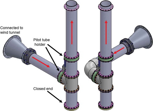
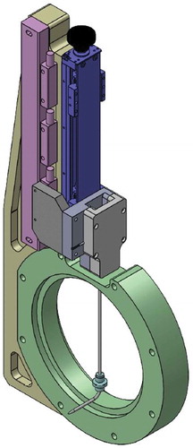
The pitot tube is held in place using a special support, equipped with a hand-controlled linear stage (Mitutoyo, Prod. Nr. 539–803) with a digital readout, allowing to accurately position the pitot tube at various radial positions in the stack. The pitot tube support is mounted to a ring of which there are two in our stack simulator (Figure 1). For an overview of the pitot tube support holder and mounting ring, see Figure 2.

Figure 2. Overview of the pitot tube support and mounting ring

The mounting rings are made such that, after loosening the bolts holding it in place, the ring is freely rotatable, allowing measurement at different measurement lines without disassembling the stack simulator. The mounting rings are placed in two positions: one just upstream of the T-junction, and the other in the vertical stack downstream of the T-junction. By using variable lengths of the pipe, the latter was placed at 3, 4, 5, 6, or 7 diameters downstream of the T-junction (as measured from the central axis of the supply pipe), to obtain five different measurement planes, which will be referred to as 3D, 4D, 5D, 6D, and 7D throughout this article. The vertical coordinates of these planes are referred to as, e.g., $z/D=3$. As only one pitot tube is used, but two mounting rings, the hole for the pitot tube on the mounting ring that is not in use, is sealed with a plug that sits flush with the inner surface of the ring. The experiments are performed with air under atmospheric pressure at temperatures of (20 ± 0.5)°C and relative humidity of (45 ± 5)%. Experiments are performed at two different volumetric flow rates, corresponding to bulk velocities $U_{bulk}=Q/A$ of 5.0 m/s and 10.0 m/s, where $Q$ denotes the volumetric flow rate and $A$ is the cross-sectional area. The wind tunnel is connected to a facility with a set of master meters, which are calibrated traceably to VSL’s primary standards. The expanded uncertainty in $Q$ does not exceed 0.15% of the reference volumetric flow rate.

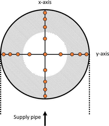
Sampling points are chosen in accordance with section 8.2 and Annex D of EN 15259 (CEN 2007), which describes the minimum number of sampling points and their position, respectively. For narrow stacks (sampling plane area less than 0.1 m²) such as our stack simulator, the standard stipulates a minimum of only 1 sampling point, which could be insufficient to get a reasonably accurate estimate of the bulk velocity in the stack. Therefore, measurements are performed at 8 sampling points per sampling line (16 points per plane), using two perpendicular sampling lines as required by the SRM (the tangential method is used). Additionally, the velocity in the center of the stack is measured to represent the situation in which one uses the minimal amount of sampling points. Thus, the axial velocity is determined in the stacks at 3.3%, 10.5%, 19.4%, 32.3%, 50.0%, 67.7%, 80.6%, 89.5%, and 96.7% of the diameter of the duct, in two lines, for the three planes 3D, 5D, and 7D. For the planes 4D and 6D, the axial velocity is determined only in the center. Note that only the points at 32.3%, 50.0%, and 67.7% of the diameter of the duct meet the requirement of the standard EN 15259 that sampling points should be at least 5 cm away from the wall. An overview of the measurement plane, lines, points, and associated definitions is given in Figure 3.

Figure 3. Top view of the measurement plane ($x$,$y$) in the stack. Orange dots represent the sampling points. The $z$-direction is perpendicular to the measurement plane. Shaded area denotes the part of the measurement plane that is less than 5 cm from the wall

The axial velocity in the stack was measured using an L-type pitot tube (AIRFLOW developments, UK), traceably calibrated in CMI’s wind tunnel. The uncertainty in the measured axial velocity $U_z$ is composed of several uncertainty sources including the pitot tube constant (calibration), differential pressure, and repeatability. The total measurement uncertainty of all measurements is calculated in agreement with the Guide to the Expression of Uncertainty in Measurement (BIPM 2008).

Computational fluid dynamics

In order to investigate the flow velocity in both configurations of the stack simulator (see Figure 1), a well-established CFD method was used. The CFD simulations were performed using OpenFOAM-5.x, free open source software containing several solvers for the turbulent flows that we are expecting in our stack (supposing fluid defined by air with kinematic viscosity 1.5 $\times$ 10⁻⁵ m²s⁻¹ Reynolds numbers reach 67,800 for $U_{bulk}=5.0$ m/s and 135,600 for $U_{bulk}=10.0$ m/s). Earlier investigations by (Geršl et al. 2018), showed limited agreement between experiment and CFD results using the so-called Reynolds Average Navier Stokes (RANS) method in stacks with a T-junction. Hence, in this study both RANS and a more precise Large Eddy Simulation (LES) method have been taken into account to obtain a more realistic flow velocity.

Geometry

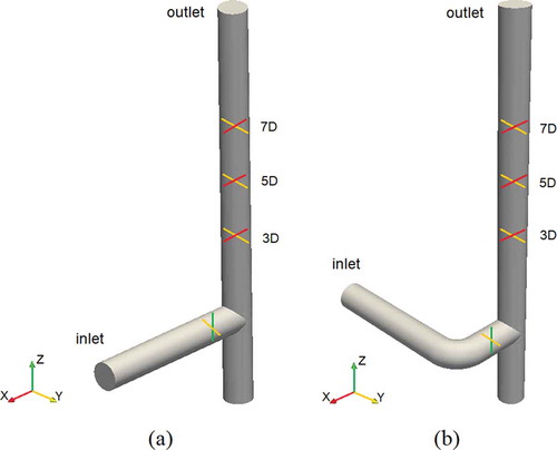
Geometrical models corresponding to the experimental stack simulators were designed for use in the CFD simulations, as can be seen in Figure 4, which also includes the measurement lines where experimental and CFD results are compared. The lines in the supply pipe to the junction are distanced 209 mm from the axis of the vertical stack. As in the experiments, the measurement planes are spaced 3, 5, or 7 diameters from the T-junction. The measurement lines in the supply pipe are oriented along the $y$- and $z$-axes, while the measurement lines in the vertical stack are oriented along the $x$- and $y$-axes. The orientation of geometries is defined so that the $x$-axis represents the reverse direction of the flow entering the T-junction and the orientation of $z$-axis represents the vertical direction in which the flow is leaving the stack.

Figure 4. Geometry of the two configurations modeled in OpenFOAM: one with a straight supply pipe (a), the other with an elbow just before the T-junction (b)

Mesh

A structured mesh was designed using the blockMesh tool (OpenCFD Ltd. 2018) implemented in OpenFOAM for both type of geometries. Several meshes were created to perform a mesh dependency study, to verify that the results are mesh independent. Note that due to the extraordinary computational demand of the LES method, only one mesh has been used in this case.

The finally chosen mesh refinement ensures for classically defined dimensionless cell thickness (CFD Online 2014): $y^{+}=1.25$, $z^{+}=40$ and $y^{+}=2.5$ and $z^{+}=80$ (23 million cells in total) for $U_{bulk}=5.0$ m/s and 10.0 m/s, respectively, for RANS simulations. The mesh refinement for LES simulation (set up only for $U_{bulk}=5.0$ m/s) was set to $y^{+}=2.5$ and $z^{+}=80$ (20 million cells in total) to conserve computational resources. For a detailed image of the mesh cross-sections, see Figure S1 of the Supplemental Material.

Numerical setting and boundary conditions

For the RANS attitude, the flow is simulated using simpleFoam, a solver for steady incompressible viscous turbulent flow implemented in OpenFOAM. Based on experience from simulations of turbulent flow in stacks (Geršl et al. 2018), the $k$-$\in$ turbulence model (Launder and Spalding 1974) was chosen in the setting of the solver. For other numerical schemes, the default combination of first and second order schemes were adopted.

The boundary conditions were defined by the classical scheme of velocity inlet and pressure outlet, i.e., a constant uniform velocity profile was set at the inlet plane and constant pressure was fixed at the outlet plane. On the walls, the no slip velocity condition was set using zero velocity and zero normal pressure gradient. The values of turbulent kinetic energy, $k$, and the rate of dissipation of turbulent kinetic energy, $\in$, were fixed at the inlet with values corresponding to the 5% turbulence intensity. The default prescriptions of the wall function have been used on the walls.

In case of the LES attitude, the large eddies (structures) in the transient flow are simulated using spatially filtered Navier-Stokes equations while the small structures are modeled using a variety of methods generally called sub-grid scale models. In order to distinguish the large and small scales an appropriate low-pass filter is used. In OpenFOAM a number of different LES packages are implemented. In this work, the Smagorinsky LES model (Smagorinsky 1963) has been used in combination with a transient pisoFoam solver for simulations of both geometries. The boundary conditions were the same as in the RANS attitude described above. In order to enhance the time averaged velocity field needed for comparison with RANS attitude, the resulting RANS velocity field was used as the initial state of the flow field. The comparison of the time averaged RANS vs. the instantaneous LES velocity field is depicted in Figure S2 of the Supplemental Material.

Validation of CFD results

CFD results have been validated by comparison of the computed axial velocity profiles with corresponding velocities experimentally measured in the sampling points defined in the Experimental section. In the case of the LES attitude, the velocity profiles are averaged over five seconds to make this comparison.

As can be seen from the velocity profiles depicted in the Supplemental Material (Figures S3--S6), both RANS and LES attitudes give similar results. While profiles on the “inlet” plane are reasonably well resolved, the agreement of CFD and experimental results is poorest in plane 3D, but is improving with increasing distance from the T-junction. Although the agreement is better for the straight supply pipe and $U_{bulk}=5$ m/s, it can be in general concluded---see also, e.g., (Walker et al. 2010) and (Ayhan and Sökmen 2012)---that the fluid behavior in the T-junction is still difficult for modeling using the classical RANS as well as the LES attitude. However, the agreement in longer distances from the T-junction is reasonable and can be used for demonstration of the flow field behavior and considerations in following sections.

Results and discussions

Resulting velocity fields

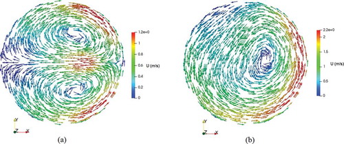
Figure 5 shows the swirl structures at a distance 3D from T-junction for the straight (a) and the elbowed (b) supply pipe. In case of the straight pipe, two counter-rotating swirls are observed, while in case of the elbowed supply pipe, only one counter-clockwise swirl is established.

Figure 5. Resulting swirl structures appearing in the stack with the straight supply pipe (a) and elbowed supply pipe (b). Cuts are in distance of 3D from T-junction. Both cases are computed using $k$-$\epsilon$ RANS attitude for $U_{bulk}$=5 m/s

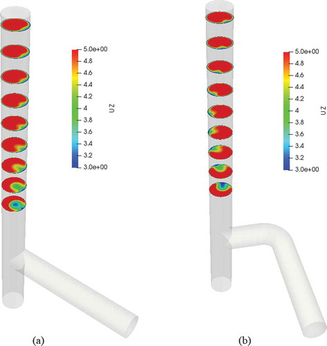
The cyclonic flow can be clearly seen in Figure 6 where the distributions of the axial velocity component are presented in cuts along the stack at several distances from the T-junction. The ($x$, $y$) location of the minimal/maximal axial velocity remains in the symmetry plane of the stack for the straight supply pipe, while counterclockwise movement is observed for the elbowed supply pipe. Although the velocity distribution is changing with distance from the T-junction, LES simulation results showed no significant temporal changes of the averaged velocity field. So, although the agreement with measurement is not perfect, as was mentioned above (see also Figures S3--S6), the RANS attitude is considered to be justified.

Figure 6. Distribution of the axial velocity component in cuts along the stack for the straight supply pipe (a) and the elbow supply pipe (b). The lowest cut is at height 3D, the highest at height 11D from T-junction

Discussion of the errors of flow measurement in stacks

Error due to flow angle sensitivity of pitot tubes

The first type of error that can occur when flow velocity is measured using pitot tubes is the error due to an angular misalignment of the pitot tube with respect to the actual flow direction in the measurement point. This error depends on how the pitot tube reacts on the angular deviations of the flow velocity vector and is different for various pitot tube types. Here we consider one representative L-type and one representative S-type pitot tube, and we discuss their possible velocity measurement errors.

Angular dependency of the L-type pitot tube

The L-type pitot tube was calibrated, and its angle dependence was measured in the wind tunnel of CMI. The pitot tube was fixed to a turntable with calibrated angle such that it could rotate around its axis given by the longer part of its L-shaped body. It was installed in the wind tunnel such that this rotation axis was always perpendicular to the air velocity vector. The inclination angle $\alpha$ was defined as the angle between the air velocity vector and the shorter sensing part of the pitot tube’s L-shaped body.

Taking the geometrical symmetry of the sensing part of the pitot tube into account we suppose that its indication depends on this inclination angle only, even if the velocity vector is not perpendicular to the longer part of its L-shape body, and therefore, the experimental configuration used gives a general angle dependence of the instrument. The pitot tube was calibrated in 15 angles α between 0° and 40° and 6 reference air velocities $U$ in the wind tunnel from 2 m/s to 15 m/s. A Laser Doppler anemometer was used as the velocity reference in the wind tunnel. The calibration coefficient of the pitot tube $C_p\left(\alpha ,U\right)$ is defined by equation

(1) $U=C_p\left(\alpha ,U\right)\sqrt{\frac{2\mathrm{\Delta }p\left(\alpha ,U\right)}{\rho }}$(1)

with $\mathrm{\Delta }p\left(\alpha ,U\right)$ being a differential pressure on the pitot tube for given angle and air velocity and $\rho$ being the air density. The coefficient $C_p\left(\alpha ,U\right)$ was determined by the measurement. The obtained results correspond well to the angle dependence of an NPL type pitot tube as published in ISO 3966 (ISO 2008); however, in our measurements we observed a dependency on the air velocity as well.

Normally, pitot tubes used in practice are calibrated in a wind tunnel with α = 0 so their calibration coefficient $C_p\left(0,U\right)$ is known only. However, when measuring in a stack, the gas flow inclination angles are typically unknown, unless non-axial flow was assessed using ISO 10,780 (ISO 1994). However, this assessment shall only be performerd if “swirl is either known to exist from previous measurements or is expected due to the geometry or stack conditions.” Therefore, the calibration coefficient $C_p\left(0,U\right)$ is used in the measurement which causes a bias if the flow in the stack is not aligned with the stack axis. If the pitot tube is installed in a stack and aligned with the stack axis and the gas velocity vector in the position of the pitot tube has an inclination α from the stack axis and magnitude $U$, the correct velocity component along the stack axis $U_{z,real}$ would be given as

(2) $U_{z,real}=Ucos\left(\alpha \right)=C_p\left(\alpha ,U\right)cos\left(\alpha \right)\sqrt{\frac{2\mathrm{\Delta }p\left(\alpha ,U\right)}{\rho }}$(2)

The measured velocity component $U_{z,meas}$ is determined as

(3) $U_{z,meas}=C_p\left(0\right)\sqrt{\frac{2\mathrm{\Delta }p\left(\alpha ,U\right)}{\rho }}$(3)

where we use $C_p\left(0\right)$considering a negligible $U$ dependence of $C_p\left(0,U\right)$. Therefore, the percentual error of the measurement of the axial velocity component by the L-type pitot tube is

(4) $E_{\alpha }=\frac{U_{z,meas}-U_{z,real}}{U_{z,real}}\times 100\mathrm{\%}=\left(\frac{C_p\left(0\right)}{C_p\left(\alpha ,U\right)cos\left(\alpha \right)}-1\right)\times 100\mathrm{\%}$(4)

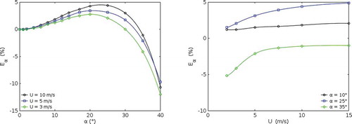
Plots of the percentual error $E_{\alpha }$ as a function of $\alpha$ and $U$ are shown in Figure 7.

Figure 7. The relative error of the L-type pitot tube as a function of the velocity inclination angle $\alpha$ and the velocity magnitude $U$

Errors of the point velocity measurement with an L-type pitot tube due to the angle $\alpha$ in the simulated gas flow in the stacks

The angle dependencies discussed in the previous section can be used to predict what would be the error of the velocity measurement by the L-type pitot tube in case of a real stack flow which is here represented by the simulated flow in the stacks with two different shapes of the supply pipe. We use the flow field from the simulation rather than the one from the experiment since the simulation gives all components of the velocity vectors which we need to determine the inclination angle. The angles $\alpha$ and the velocities $U$ have been determined from the simulations at the experimental measurement locations in the stack and the corresponding pitot tube error has been calculated according to equation (4)(4) $E_{\alpha }=\frac{U_{z,meas}-U_{z,real}}{U_{z,real}}\times 100\mathrm{\%}=\left(\frac{C_p\left(0\right)}{C_p\left(\alpha ,U\right)cos\left(\alpha \right)}-1\right)\times 100\mathrm{\%}$(4) using two-dimensional linear interpolation of the measured $E_{\alpha }\left(\alpha ,U\right)$ dependence.

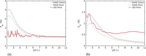
Since the angles are relatively small (typically smaller than 10° in the center line of stack), as can be seen in the Supplemental Material (Figures S3--S6), the resulting errors are also relatively small. The percentual errors of the velocity measurement by the L-type pitot tube due to the angle $\alpha$ in the center of the stack are depicted in Figure 8, as a function of the distance from the T-junction. As can be seen from the graphs, the errors are less than 2% for both geometrical configurations. The errors for other measurement locations (see Figure 3, where $\alpha$ can reach 30° in sampling points close to walls) do not exceed 4%.

Figure 8. Relative errors of axial velocity measurement by the L-type pitot tube in central axis ($x=0$,$y=0$) of the stacks due to the angle$\alpha$. Stack with straight (a) and elbowed (b) supply pipe

Angular dependency of an S-type pitot tube

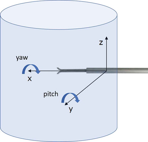
Although this article is focused on L-type pitot tube measurements, for comparison, the corresponding errors for measurements with the commonly used S-type pitot tube are shown in the following sections. Due to the asymmetric shape of the S-type pitot tube, velocity measurements depend on the orientation of the pitot tube to the velocity field defined by its yaw and pitch angles (Muzio et al. 1996). Yaw angle, $\beta$, is defined as the angle between the $z$-axis and the projection of the velocity vector to the $\left(y,z\right)$ plane (see Figure 9). Pitch angle, $\gamma$, is defined as the angle between the velocity vector and the $x$-axis minus 90° (see Figure 9).

Figure 9. Visual representation of the yaw ($\beta$) and pitch ($\gamma$) angle of an S-type pitot tube

The relative measurement error (as a percentage) of one of the S-type pitot tubes tested in (Muzio et al. 1996) depending on the yaw and pitch angles (in degrees) can be approximated by (Geršl et al. 2018):

(5) $E_{\beta ,\gamma }=\left(a_1{\gamma }^2+a_2\gamma +a_3\right){\beta }^2+c_1{\gamma }^2+c_2\gamma$(5)

where $a_1=1.4\times {10}^{-5}$, $a_2=4.5\times {10}^{-4}$, $a_3=0.024$, $c_1=5.9\times {10}^{-3}$, and $c_2=0.13$.

Errors of the point velocity measurement with S-type pitot tube due to the yaw and pitch angles in the simulated gas flow in the stacks

The errors according to equation (5)(5) $E_{\beta ,\gamma }=\left(a_1{\gamma }^2+a_2\gamma +a_3\right){\beta }^2+c_1{\gamma }^2+c_2\gamma$(5) were computed for two installation directions of the S-type pitot tube and for both types of stacks. In the first case, the pitot tube is installed along the -$x$ axis of the stack (see Figure 4), while in the second case it is along the $y$ axis. The resulting relative errors for both installation directions are depicted in Figures 10 and Figure 11, respectively. The errors in the stack with elbowed supply pipe are less than 2% for $z/D$ larger than 3 for both installation directions and both simulation attitudes.

Figure 10. Relative errors of the velocity measurement with the S-type pitot tube in central axis ($x=0$,$y=0$) of the stacks with straight supply pipe (a) and with the elbowed supply pipe (b); pitot tube along the $x$-axis of the stack

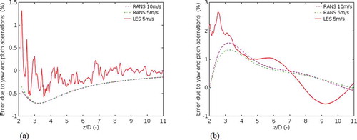
Figure 11. Relative errors of the velocity measurement with the S-type pitot tube in central axis ($x=0$, $y=0$) of the stacks with straight supply pipe (a) and with the elbowed supply pipe (b); pitot tube along the $y$-axis of the stack

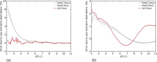
In case of the stack with straight supply pipe, the error is less than 2% with the pitot tube installed along the $x$-axis, while in case of the installation along the $y$-axis the maximal errors have larger differences between the RANS and LES flow field models for smaller distances from the T-junction. However, for both installation directions of the S-type pitot tube, the resulting errors are consistent in the sense that the errors decrease with increasing distance from T-junction due to homogenization of the flow field as can be seen in Figure 6a. This is not the case for the elbowed supply pipe where the resulting swirl remains alive along the whole $z$-axis of the stack, see Figure 6b, and causes the corresponding yaw and pitch errors.

Error of flow rate determination due to selection of sampling points for velocity measurement

After the axial velocity of a gas in a stack is measured in one or several points in a grid prescribed by the EN 15259 standard, the measured flow rate is determined as $Q_m=A\cdot U_r$ with $A$ being the stack cross-sectional area and $U_r$ being a representative velocity given as an average of the measured velocities. The real flow rate, on the other hand, is given as $Q=A\cdot U_{bulk}$ with $U_{bulk}$ being an average axial velocity component all over the cross-section of the stack. The value of $U_r$ depends on position and number of the selected sampling points and the difference between $U_r$ and $U_{bulk}$ causes an error in flow rate measurement given as

(6) $dQ=A\cdot \left(U_r-U_{bulk}\right)$(6)

Combining equation (6)(6) $dQ=A\cdot \left(U_r-U_{bulk}\right)$(6) with the equation for the real flow rate ($Q=A\cdot U_{bulk}$), the following expression for the relative error of flow rate measurement is obtained as follows:

(7) $E_{total}=\frac{dQ}{Q}=\frac{U_r-U_{bulk}}{U_{bulk}}$(7)

Note that, since $U_r$ is measured with a pitot tube which suffers from flow angles errors as discussed in previous sections, the error $E_{total}$ depicted below in Figures 12 and Figure 13 includes both the error due to the selection of sampling points and inherently the flow angle error $E_{\alpha }$.

Figure 12. Relative error of flow rate determined from one sampling point in the center ($U_r\equiv U_{center}$) of stack cross-section in a stack with straight supply pipe (a) and with the elbowed supply pipe (b). Uncertainty bars represent the (total) flow measurement uncertainty (k = 2) of the experiment

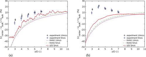
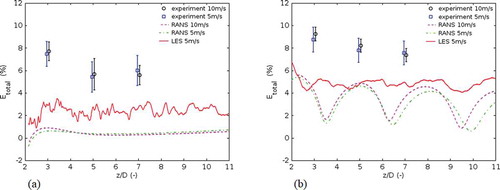
Figure 13. Relative error of flow rate determined from 16 sampling points in a stack with straight supply pipe (a) and with the elbowed supply pipe (b). Uncertainty bars represent the (total) flow measurement uncertainty (k = 2) of the experiment

Error of flow rate determination in case of one sampling point in the stack center

As written in the Introduction, only one measuring point is required according to the current SRM referring to EN 15259 for flow rate measurement in narrow stacks. Supposing the point is located in the center of stack cross-section, varying values of $U_r\equiv U_{center}$ can be expected for non-uniform velocity profiles depending on the influence of turbulent mixing close to the T-junction and the development of the velocity profile along the pipe.

Figure 12 shows the relative error as defined by equation (7)(7) $E_{total}=\frac{dQ}{Q}=\frac{U_r-U_{bulk}}{U_{bulk}}$(7) in stacks with straight and elbowed supply pipe. Data from the stack simulator experiment at VSL and the CFD simulations performed at CMI are included. As can be expected from the velocity profiles shown in the Supplemental Material, RANS and LES simulations give similar results for both type of geometries.

In case of the straight supply pipe, the relative error determined from the experiment ranges from about −10% for $z/D=3$ to about +10% for $z/D=11$. The relative error determined from CFD takes values from about −30% to about +10%. The behavior of errors given by CFD and experiment is very similar and is expected from the development of the turbulent velocity profile in the vertical part of the stack. It is noteworthy that for a fully developed turbulent flow profile in pipes (Gersten 2005), the calculated error is approximately 20% (depending on Reynolds number), as the velocity in the center exceeds the average value. Hence, both the CFD simulations and the experimental results approach this value when increasing $z/D$, rather than zero.

In case of the elbowed supply pipe, the relative error determined from CFD increases from about −20% for $z/D=3$ to about +10% for $z/D=11$. In this case the behavior of the RANS and LES simulations differ in the sense that for LES the maximal axial velocity is reached at $z/D=7$, so errors do not exceed about 6% further downstream. The error indicated by RANS does slightly increase beyond this value over the whole length of the vertical stack. The relative error determined from the experiment ranges from about +10% for $z/D=3$ to about +10% for $z/D=7$ with the maximum roughly at $z/D=4$ where the error reaches about 20%. The differences observed between experiment and CFD simulations are attributed to the inaccurate modeling of mixing in the T-junction part, as experiments and CFD results are getting closer with increasing $z$-coordinate.

Error of flow rate determination in case of 16 sampling points

A logical way to improve flow rate measurement accuracy is to increase the number of sampling points. In the experiments, the appropriate measurements were done using grid sampling as described in the experimental section. Hence, similar graphs as in Figure 12 have been made for $U_r$ computed from the remaining 16 sampling points, i.e., all points except the central one as depicted in Figure 3. These sampling points are spaced according to the tangential method of EN 15259, which is required by the SRM. However, only 4 out of 16 points meet the additional requirement of being more than 5 cm away from the wall. The representative velocity is given as the average of axial velocity components in 16 sampling points:

(8) $U_r\equiv 1/16\cdot \sum _{i=1}^{16}{U}_{z,i}$(8)

As can be read from Figure 13, like in the case of the single sampling point of Figure 12, the mean velocities given by simple averaging of 16 axial velocities computed by RANS as well as LES attitude are lower than the corresponding experimental values for both stack geometries. Similar to Figure 12, the LES attitude gives slightly better agreement with experiment. In the case of the elbowed supply pipe, RANS predicts an influence of swirl while this is not reproduced by LES. Unfortunately, as no grid measurements were performed at 4D and 6D, experimental data is not available to shed more light on this discrepancy.

In both cases, the errors of calculated flow rate given by 16 points are about half of the errors based on a single sampling point in the center. As can be read from Figure 13, the errors in both cases range from about 5% to 10% compared to about 10% to 20% in Figure 12.

Not only is the measurement using grid sampling more accurate (lower absolute error), the measurement uncertainty is also reduced, as indicated by the difference in size of the error bars between Figures 12 and Figure 13 (taking into account the difference in scale on the vertical axis). This is because the uncertainty of the average value can be approximated by the average value of the uncertainties of measurements in all sampling points, divided by the square root of the number of sampling points, given that the individual measurements have similar uncertainties (which is the case here). Due to the nature of our experimental setup, the single sampling point in the center was measured four times, and hence the uncertainty for the grid measurement (16 points) roughly equates to $\sqrt{4}/\sqrt{16}=1/2$ the value of the single sampling point. For a more typical measurement campaign with only one measurement, this ratio would be $1/4$.

Note that, apart from the measured velocity $U_r$, also the measurement of the cross-sectional area $A$ affects the error of the measured flow rate ($Q_m=A\cdot U_r$). In our experiments, we determine the expanded uncertainty of the measurement of the cross-sectional area to be 2%. Hence, the measurement of $Q_m$ is affected mostly by the error in $U_r$. Note that the cross-sectional area is slightly reduced due to the insertion of the Pitot tube; however, this effect is negligible here (using an L-type pitot tube). For a similarly sized S-Pitot tube, however, the effect may also be about 2%.

Conclusion

In this article, two different sources of error of flow rate measurement in stacks have been investigated assuming the flow rate is measured according to the Standard Reference Method (EN ISO 16911–1) using pitot tubes in a grid of points. The error due to a pitot tube sensitivity to inclined flow direction and the error due to number and position of the sampling points have been discussed. Two distinct stack geometries have been used to investigate how different flow disturbances and swirl can influence the errors.

The flow velocity in the two geometries was studied experimentally in a stack simulator and was simulated with CFD software OpenFOAM using RANS and LES attitudes. Time averaged velocity profiles in defined sections from CFD were compared to the experimental data. The comparison shows that even the more precise LES method has difficulties in the correct modeling of the flow near the T-junction. However, the agreement of the resulting computed velocity profiles with experimental results is acceptable with increasing distance from T-junction, especially for lower bulk velocity, and can serve as a basis for discussion of the flow rate measurement errors.

The first type of error discussed in the article, which relates to the flow inclination with respect to a pitot tube, e.g., due to swirl, was discussed for both L-type and S-type pitot tubes with different angular dependencies. The angular dependency of the L-type pitot tube was measured in a wind tunnel and applied to predict its error when used for a velocity measurement in the considered stacks. Using the computed flow velocity and corresponding angles inside the studied stacks it was reported that this kind of error is typically smaller than 2% in case the sampling point is in the center of the cross-sectional area and less than 4% for the other experimental sampling points.

In case of S-type pitot tube, the influence of yaw and pitch angles was discussed using an empirical equation from literature. Two configurations of the S-type pitot tube positioning were studied. For both configurations and both stack geometries the errors caused by yaw and pitch angles were less than about 2% for $z/D$ larger than 3. Thus, both type of pitot tubes have comparable sensitivity to the flow angle.

The second type of error discussed in this article relates to the number and position of sampling points used for the flow rate measurement. This type of error is significantly larger than the error due to flow angle. The errors occurring in flow rate measurements using one sampling point located in the center of the stack can reach 10% and 20% for stack with straight supply pipe and elbowed supply pipe, respectively. The errors using 16 sampling points according to the tangential method for grid sampling (according to EN 15259) are about two times smaller, i.e., 5% and 10%, even though most of these sampling points do not meet the requirement of EN 15259 of being more than 5 cm away from the wall.

Note that for both stack geometries, i.e., shapes of the supply pipe, both types of errors seem to be independent of the bulk velocity (see Figures 8 and Figure 10–Figure 13). Thus, the results presented in this article are considered to have universal value for stacks with Reynolds numbers of similar order of magnitude as studied here. The minimal requirements of the SRM of having one sampling point for narrow ducts and five or more hydraulic diameters straight duct upstream from the sampling plane, does not exclude potential errors around 10% and 15% for straight and elbowed supply pipe, respectively.

Based on the results presented in this article, it can be concluded that both the number and location of sampling points need an appropriate assessment, also considering the shape of supply pipe. Carefully selecting sampling points can yield significant reductions in errors, making the enforcement of the increasingly small emission limit values more reliable.

Acknowledgment

Helpful discussions with Rod Robinson and Richard Dwight are gratefully acknowledged. Thomas Smith is acknowledged for his help proofreading this work. This work is part of the EMPIR 16ENV08 project “Metrology for air pollutant emissions.” This project (16ENV08) has received funding from the EMPIR program co-financed by the Participating States and from the European Union’s Horizon 2020 research and innovation program.

Disclosure statement

No potential conflict of interest was reported by the authors.

Supplementary material

Supplemental data for this article can be accessed on the publisher’s website

Additional information

Funding

This work was supported by the European Association of National Metrology Institutes [EMPIR / 16ENV08]; Ministerstvo Školství, Mládeže a Tělovýchovy (MŠMT ČR).

Notes on contributors

Stanislav Knotek

Stanislav Knotek, Ph.D., is a metrologist at Czech Metrology Institute, Brno, Czech Republic.

Marcel Workamp

Marcel Workamp, Ph.D., is a scientist at VSL Dutch Metrology Institute, Delft, The Netherlands.

Jan Geršl

Jan Geršl, Ph.D. is a metrologist at Czech Metrology Institute, Brno, Czech Republic.

Menne D. Schakel

Menne D. Schakel, Ph.D., is a scientist at VSL Dutch Metrology Institute, Delft, The Netherlands.

References

- Ayhan, H., and C. N. Sökmen. 2012. CFD modeling of thermal mixing in a T-junction geometry using LES model. Nucl. Eng. Des. 253:183–91. doi:10.1016/j.nucengdes.2012.08.010.
- BIPM. 2008. GUM: Guide to the expression of uncertainty in measurement. https://www.bipm.org/en/publications/guides/gum.html.
- CEN. 2007. EN 15259: Air quality---Measurment of stationary source emissions---Requirements for measurement sections and sites and for the measurement objective, plan and report. CEN.
- CEN. 2013a. EN ISO 16911–1:2013: Stationary source emissions---Manual and automatic determination of velocity and volume flow rate in ducts---Part 1: Manual reference method. CEN.
- CEN. 2013b. EN ISO 16911–2:2013: Stationary source emissions---Manual and automatic determination of velocity and volume flow rate in ducts---Part 2: Automated measuring systems. CEN.
- CFD online. 2014. Dimensionless wall distance (y plus). Accessed April 8, 2020. https://www.cfd-online.com/Wiki/Dimensionless_wall_distance_(y_plus).
- Dimopoulos, C., R. A. Robinson, and M. D. Coleman. 2017. Mass emissions and carbon trading: A critical review of available reference methods for industrial stack flow measurement. Accredit. Qual. Assur. 22 (3):161–65. doi:10.1007/s00769-017-1261-0.
- European Commission. 2003. Directive 2003/87/EC of the European parliament and of the council of 13 October 2003 establishing a system for greenhouse gas emission allowance trading within the Union and amending Council Directive 96/61/EC. European Commission.
- European Commission. 2010. Directive 2010/75/EU of the European parliament and of the council of 24 November 2010 on industrial emissions (integrated pollution prevention and control). European Commission.
- European Commission. 2015. Directive 2015/2193 of the European parliament and of the council of 25 November 2015 on the limitation of emissions of certain pollutants into the air from medium combustion plants. European Commission.
- Fowler, D., K. Pilegaard, M. A. Sutton, P. Ambus, M. Raivonen, J. Duyzer, and D. Simpson. 2009. Atmospheric composition change: Ecosystems-atmosphere interactions. Atmos. Environ. 43 (33):5193–267. doi:10.1016/j.atmosenv.2009.07.068.
- Geršl, J., S. Knotek, Z. Belligoli, R. P. Dwight, R. A. Robinson, and M. D. Coleman. 2018. Flow rate measurement in stacks with cyclonic flow - Error estimations using CFD modelling. Measurement 129:167–83. doi:10.1016/j.measurement.2018.06.032.
- Gersten, K. 2005. Fully developed turbulent pipe flow. In Fluid mechanics of flow metering, edited by W. Merzkirch, 1–22. Berlin: Springer-Verlag Berlin Heidelberg.
- ISO. 1994. ISO 10780: Stationary source emissions—Measurement of velocity and volume flowrate of gas streams in ducts. ISO.
- ISO. 2008. ISO 3966: Measurement of fluid flow in closed conduits—Velocity area method using Pitot static tubes. ISO.
- Kampa, M., and E. Castanas. 2008. Human health effects of air pollution. Environ. Pollut. 151 (2):362–267. doi:10.1016/j.envpol.2007.06.012.
- Launder, B. E., and D. B. Spalding. 1974. The numerical computation of turbulent flows. Comput. Methods Appl. Mech. Eng. 3 (2):269–89. doi:10.1016/0045-7825(74)90029-2.
- Muzio, L. J., T. D. Martz, R. D. McRanie, and S. K. Norfleet. 1996. Flue gas flow rate measurement errors. Oak Ridge: U.S. Department of Energy.
- OpenCFD Ltd. 2018. The open source CFD toolbox. Open source software. Accessed May 5, 2020. https://www.openfoam.com/documentation/user-guide/blockMesh.php.
- Smagorinsky, J. 1963. General circulation experiments with the primitive equations I. The basic experiment*. Mon. Weather Rev. 91 (3):99–164. doi:10.1175/1520-0493(1963)091<0099:GCEWTP>2.3.CO;2.
- Walker, C., A. Manera, B. Niceno, M. Simiano, and H.-M. Prasser. 2010. Steady-state RANS-simulations of the mixing in a T-junction. Nucl. Eng. Des. 240 (9):2107–15. doi:10.1016/j.nucengdes.2010.05.056.