Gridded bias correction of modeled PM_2.5 for exposure assessment, and estimation of background concentrations over a coastal valley region of northwestern British Columbia, Canada

ABSTRACT

Chemical transport models (CTM) can have large biases and errors when simulating pollutant concentrations. To improve the characterization of fine particulate matter (PM_2.5) over complex terrain for exposure assessments, three mathematical formulae that utilized the relationship between modeled and observed quantile concentrations at a monitor location were developed. These were then applied to 1 year of CMAQ model output of PM_2.5 over the Terrace–Kitimat Valley of northwestern British Columbia, Canada. The final products enhanced the representation of ambient levels at existing monitoring stations when evaluated with conventional statistical measures. Better agreement of corrected outputs with observed compliance metrics was also found. On average, the absolute errors of amended outputs were 11% and 10% for the annual mean PM_2.5 and 98th percentiles of daily concentrations, respectively, compared to 45% and 61%, respectively, in the original outputs. These improvements provided greater confidence to use the amended outputs to estimate concentrations at locations without monitors. The predominance of pristine conditions in the modeling domain was exploited to derive annual background PM_2.5 concentrations over the valley, which was estimated to be 2.0–2.3 μg m⁻³. To our knowledge, this is the first study to calculate background PM_2.5 concentrations over northern BC coastlands using bias-corrected outputs from an air quality model.

Implications: Bias correction of CMAQ model output was necessary for assessing regulatory compliance for ambient PM_2.5. The implications are notable. First, for low to moderate spatial heterogeneity in monitoring data, the use of regression equations that relates quantile mean concentrations of model outputs to those of observational data enhances the estimation of PM_2.5 at unmonitored locations. Second, by providing spatial pollutant distribution ahead of planned industrial development in Terrace–Kitimat Valley (TKV), corrected model output offers a baseline for tracking progress in airshed management. Third, correction improved pollutant exposure classification, for which the risk was predominantly low. Finally, 2.0–2.3 μg m⁻³ should be considered as PM_2.5 concentrations that are irreducible when setting voluntary targets for ambient levels in the area.

Introduction

Air pollution due to particulate matter with an aerodynamic diameter ≤2.5 µm (PM_2.5) is a widely acknowledged threat to human health. Exposure to PM_2.5, which may be released from natural and human activities such as wildfires and residential wood heating, has been associated with adverse health effects, notably heart and lung impairment (Atkinson et al. 2015; Crouse et al. 2012). WHO (2016) estimates that globally in 2012, outdoor (ambient) PM_2.5 was responsible for about 3 million deaths in urban and rural areas. Because of morbidity and mortality impacts, regulations by various jurisdictions to limit ambient levels are stringent, with ambient monitoring focused mainly on cities. Investigations (e.g. Crouse et al. 2012) have also associated early deaths to long-term exposure to PM_2.5 concentrations lower than previously thought to be harmful. Consequently, there is growing interest in quantifying pollutant exposure in the backcountry where there often is little monitoring, and underlying problems could remain undetected for long periods.

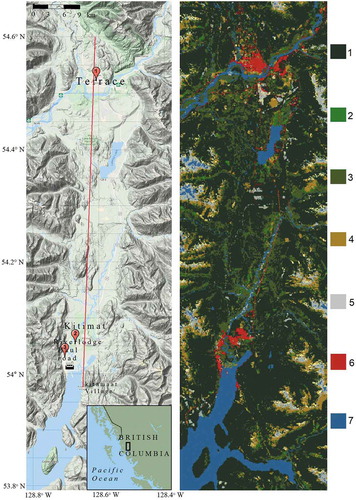
The Terrace–Kitimat Valley is a deep, narrow valley in the coast mountain ranges of northwestern British Columbia, Canada (Figure 1). It has a wet climate, with the months of November to March marked by heavy snowfall (Environment and Climate Change Canada 2019). About 28,000 people live in the valley (Statistics Canada 2018) of which a large majority are in and around the small city of Terrace and the port town of Kitimat. Historically associated with acceptable air quality, recent industrial emissions permitting, and plans for rapid industrialization in the valley have raised concerns about potential air quality impacts, and population exposure to ambient PM_2.5 (Environmental Appeal Board 2015; ESSA Technologies, Risk Sciences International, and Trinity Consultants 2015). An aluminum smelter in Kitimat has been permitted to increase its pre-2014 emissions limit of sulfur dioxide—a precursor of secondary-formed PM_2.5—by 56 % (Environmental Appeal Board 2015).  In addition, several proposed export processing facilities such as for liquefied natural gas (District of Kitimat 2019), would when operational, emit fine particles.

Figure 1. (Left) The Terrace–Kitimat valley (TKV) in the Coast Mountains of northwestern British Columbia, Canada. PM_2.5 monitoring stations are indicated with red markers, with an aluminum smelter (factory icon) located just south of the Haul Road Station. The red line is a transect denoting valley centerline used in this study. (Right) land cover types over the TKV: 1. Temperate needleleaf forest, 2. Temperate broadleaf deciduous forest, 3. Mixed forest, 4. Temperate shrubland, 5. Barren land, 6. Urban and built-up, 7. Water

The British Columbia (BC) Ministry of Environment and Climate Strategy has the mandate of regulating air emissions throughout the province, including developing standards and objectives on air quality that is protective of public health. They also partner with local communities in recommending planning goals for airsheds, particularly in defining desirable, voluntary limit values for ambient PM_2.5 in the face of economic growth and development. However, goal-setting and overall airshed management in the TKV present some challenges. First, fixed-site pollutant monitoring stations are few and likely unrepresentative of ambient levels over much of the area. Second, despite their regulatory intent, the realism of air quality models in quantifying present pollutant levels is unknown. Past air quality modeling in the area (e.g. ESSA Technologies, Risk Sciences International, and Trinity Consultants 2015) focused on predictions of contaminant concentrations arising from emission changes. However, without establishing existing pollutant concentration, it will be difficult to account for cumulative emission impacts and tracking progress in airshed management. Third, PM_2.5 modeling may exhibit discrepancies from observations that excessively underrate or exaggerate the concentration of particulate pollution over an area. Unless bias correction (Neal et al. 2014; Porter et al. 2015) is performed, model outputs may misclassify ambient PM_2.5 exposures. Finally, there is a need to discriminate particulate levels that can be reduced from those that are due to natural emissions within the airshed plus sources from outside of it. The irreducible levels, more appropriately referred to as background concentrations (McKendry 2006; Veira et al. 2013), is a vital element for consideration when setting out air quality goals and mobilizing resources to achieve them.

Bias correction for PM_2.5 has evolved alongside needs for operational forecasting and public alert systems, and statistics-based approaches, such as moving means (Djalalova, Delle Monache, and Wilczak 2015), Kalman filter (Borrego et al. 2011; Kang, Mathur, and Rao 2010) and analog correction (Huang et al. 2017) are common. Notwithstanding, adjustment of model concentrations in hindsight mode, is key to air quality attainment demonstrations and exposure assessments. Porter et al. (2015) proposed four methods to adjust for model bias and errors in order to provide greater confidence for such uses. But apart from quantitative correctness, spatial variation of PM_2.5 needs to be represented adequately. This consideration is pertinent to BC where regulatory compliance of an air basin is often assessed with measurement data from a single monitoring station (BCMOE 2017) and background contributions within may vary seasonally.

In this manuscript, objective bias-correction techniques for CMAQ-modeled PM_2.5 over the TKV, for the purpose of deriving ambient exposure and background concentrations, are developed and implemented. The aspect of generating realistic concentrations of this pollutant at unmonitored locations, and in essence, estimating compliance to air quality standards are addressed. The questions that are dealt with are (1) What bias corrections may suffice for quantifying PM_2.5 throughout the TKV? (2) How does corrected model output characterizes the spatial distribution of PM_2.5? (3) How reliable are corrected outputs for qualifying ambient PM_2.5 exposure? (iv) What irreducible concentration may be considered in setting voluntary targets for PM_2.5? The remainder of this manuscript is organized as follows. In the “Methods” section, we describe data types, retrieval, and utilization for the development of corrective schemes, and analytical methods. In the “”Results and analysis” section, the bias-correctedresults are compared with the original model outputs and with observations, also assessing the extent to which refined outputs capture indices of local regulatory compliance. In addition, background concentrations in the area are derived. The “Discussion” section discusses the relevance of final gridded concentrations for present and future airshed management. The “Summary and conclusion” section summarizes and concludes the paper.

Methods

Model simulations and observations data

We provide a brief description of the modeled and observational data used in this study. The reader is referred to Onwukwe and Jackson (2020a) for additional details. A full year (2017) of PM_2.5 concentrations was simulated off-line, over the TKV and surrounding areas using the WRF-SMOKE-CMAQ modeling platform (Appel et al. 2018; Skamarock et al. 2019; UNC 2009). Simulations were run on a 36 × 106, 1-km horizontal resolution grid for different meteorological driver options. PM_2.5 outputs used in this study are from runs with the Mellor–Yamada–Nakanishi–Niino level 3 planetary boundary-layer scheme, which demonstrated the closest match with observations. The observations are valid hourly records from three PM_2.5 monitoring stations (Table 1) for the same year of simulations and are available at https://envistaweb.env.gov.bc.ca/DynamicTable2.aspx?G_ID=327. Observational data completeness across stations were mostly >90% at seasonal intervals. For this study, seasons are defined as March–May (spring), June–August (summer), September–November (autumn), and December–February (winter).

Table 1. PM_2.5 monitoring locations, and hourly observation data completeness for the year 2017, to the nearest percentage (%)

Station	Latitude ° N	Longitude ° W	Spring	Summer	Autumn	Winter	Total
Terrace	54.522	128.608	100	96	98	62	89
Riverlodge	54.054	128.671	100	99	99	100	100
Haul Road	54.029	128.702	97	98	98	99	98

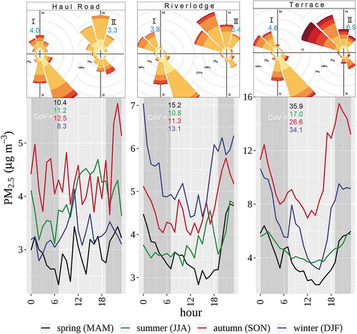
Observational data indicate that the summer season has the best correlation (r) of daily mean PM_2.5 concentrations between stations, followed by the spring season (Table 2). Sea-land breezes and along-valley circulations as well as convective mixing prevail during the warm summer months (Onwukwe and Jackson 2020b) and propagate similar PM_2.5 concentrations, hence the relatively high spatial correlation of pollutant concentration among the three stations. In colder months (autumn and winter seasons), inversions are more frequent and the decoupling of atmospheric layers aloft from the surface is more prolonged. Importantly, ambient PM_2.5 is more spatially variable due to differing intensities of cold air pools, dissimilarity of local emissions, and the relative position of stations and pollutant sources to prevailing winds. The amplitudes of PM_2.5 diurnal profiles, especially in autumn and winter (Figure 2), suggest location as more preeminent than regional forcing for pollutant variability (also, Appendix A). The Riverlodge monitor, for instance, is more impacted by local residential wood combustion sources of PM_2.5 during winter than is the Haul Road station since both are upwind of the principal industrial source (Rio Tinto Aluminum smelter) at this time of the year. It is for this reason that wintertime r value between station pairs is smallest for the two locations, despite being within 3 km of each other.

Table 2. Pearson’s correlation coefficients (r) and coefficients of divergence (CoD), for daily average PM_2.5 between station pairs in 2017

Statistic	Station pairs	Spring	Summer	Autumn	Winter	All year
r	RVL/HRD	0.48	0.89	0.38	0.23	0.51
	TER/HRD	0.38	0.79	0.23	0.39	0.39
	TER/RVL	0.45	0.82	0.71	0.67	0.65
COD	RVL/HRD	0.21	0.18	0.29	0.33	0.26
	TER/HRD	0.27	0.23	0.50	0.39	0.36
	TER/RVL	0.21	0.20	0.40	0.22	0.28

RVL, HRD, TER are Riverlodge, Haul Road and Terrace, respectively. The formulas of r and CoD are in Appendix B.

Figure 2. Seasonal distribution of PM_2.5 in the TKV. Top: Pollution roses for summer (I) and winter seasons (II) at monitoring stations. Seasonal averages (in μg m⁻³) are in blue. Bottom: Average of hourly PM_2.5 concentrations and their coefficients of variation (CoV). CoV is the standard deviation of hourly concentrations divided by the diurnal mean

Better agreement across stations for summertime ambient PM_2.5 levels also translates to measurements that are spatially more homogeneous in this season than in the others, as inferred from the coefficients of divergence (CoD, Table 2) which is a useful index for characterizing PM_2.5 uniformity in space (e.g. Ghim, Chang, and Jung 2015; Krudysz et al. 2009; Wilson et al. 2005). The CoD values for spring are slightly greater than those of summer but less than those of the autumn and winter seasons. Except for summertime for the Riverlodge/Haul Road pair, station pairs have CoD values between 0.20 and 0.50. CoD <0.2 describes relative homogeneity, 0.2–0.6 is moderate heterogeneity while >0.6 represents strong heterogeneity (Ghim, Chang, and Jung 2015; Pinto, Lefohn, and Shadwick 2004). Hence, ambient PM_2.5 distribution in the study area can be described as moderately heterogeneous in space.

Prior evaluations (Onwukwe and Jackson 2020a) indicated significant differences between modeled and observed PM_2.5 levels. Specifically, quantile distributions showed that the model underestimates the mean of the top quantiles by factors >2. The errors in modeling that result in the need for bias correction are from two main sources. The first comes from the inexactness of the emission inventory (amount, location, characteristics and configuration of emission sources) – this directly impacts the modeled ambient levels. The other is associated with how well the model itself emulates atmospheric processes, which includes the representation of meteorological variables, and transport, dispersion, and transformation of pollutants. Consequently, an adjustment of concentration distribution in the original output is necessary to ameliorate the above shortcomings. The original model representation of observations (see Figure 3) is the basis for bias correction that is explained next.

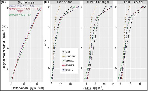
Figure 3. (a.) Regression plots of quantile mean concentrations of the original model output against those of observational data at Terrace, and derivation of bias-correction formulae. Small open circles are the data points for both (b.) Quantile plot for modeled and observed (OBS) data at pollutant monitoring stations. The concentration at each octile is the mean of all hourly concentration values within that octile. SIMPLE, POWER and DEG_2 are post-correction profiles

Bias-correction formulations

Three separate mathematical equations relating observations to simulations are derived and analyzed for their effect on the original output and they are (1) simple linear regression (2) power transformation (Li 2005) of the dependent variable in (1) based on a maximum likelihood parameter; and (3) second-degree polynomial. Figure 3a describes the three correction models. The equations are derived from data for the Terrace station and applied to estimate PM_2.5 concentrations for the entire TKV area. This choice for training the mathematical correction models is because the Terrace station demonstrates the strongest PM_2.5 diurnal variation (Figure 2), reports the highest pollutant concentrations (Figure 3b), is affected by diverse pollutant sources (road dust, vehicular traffic, residential sources, etc.); and it is located in an area of significant terrain complexity (deep-lying urban observatory). Half the dataset is used to create the equation for Terrace using values from every second day, and the remaining data is used for evaluations at this station. All hourly observations at the Riverlodge and Haul Road stations are used for evaluation. Each of the equations is applied to the original hourly output for the entire grid to generate domain-wide corrections. In the rest of this paper, “ORIGINAL” refers to the original model output, while “SIMPLE”, “POWER” and ‘DEG_2ʹ refers to correction models (1), (2) and (3), respectively.

Evaluation measures

Standard statistical measures namely normalized mean bias (NMB), normalized mean square error (NMSE), and proportion of model results within a factor of two of observations (FAC2) to assess whether, and to what extent the final products reduce original biases. Several authors (e.g. Chang and Hanna 2004; Solazzo and Galmarini 2016) recommend these statistics for model performance evaluations and their formulae are listed in Table 3. NMB and NMSE are bounded between zero and infinity, and values closer to zero are desired. Benchmarks for good model performance (Chang and Hanna 2004) are also indicated. The assessment of modeled-observation data pairs is done for daily averaged data per season, following recommendations of Emery et al. (2017) for modeling of PM_2.5. Bias-corrected products are also evaluated for fitness with prevailing air quality objectives. Statistics for the latter are summarized as mean errors (ME), and also in a conformity plot (Figure 4).

Table 3. Statistical measures for bias-correction evaluations. In the formulae, M_i is modeled/corrected concentration, with corresponding observation O_i, while $\bar{\mathrm{M}}$($\bar{\mathrm{O}}$) are their respective means. Overbar denotes computation of a mean value

Measure	Formula	Performance
		Ideal	Recommended
FAC2	-	100%	50%
NMB	$\frac{\bar{\mathrm{M}}-\bar{\mathrm{O}}}{\bar{\mathrm{O}}}$	0	±0.3
NMSE	$\frac{\overline{{(\mathrm{M}\mathrm{i}-\mathrm{O}\mathrm{i})}^2}}{\bar{\mathrm{M}}\bar{\mathrm{O}}}$	0

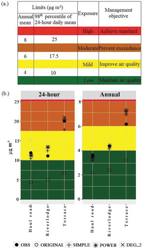
Figure 4. Top: Tiered air management threshold values and actions for ambient PM_2.5 adapted to British Columbia from (CCME 2012). Bottom: Conformity of original and corrected outputs to observed CCME 2012 PM_2.5 management categories

Results and analyses

Accuracy of bias-corrected outputs

The quantile mean concentrations of bias correction vis-à-vis original simulation and observations across stations are shown in Figure 3b. The main effect of the regression schemes is to shift the distribution profiles closer to observation. Biases for top concentrations are reduced. However, mixed outcomes are evident; the mean of the top quantile remains underestimated at Haul Road but overestimated at the other two stations. The commonality of overestimation for the Terrace station (that is used for deriving the corrections) and the Riverlodge station could be due to a similar pattern of PM_2.5 variability (Figure 2), wherein hours of low and high levels at the two stations are quite distinct. Their locations are influenced by residential PM_2.5 emissions, unlike at the Haul Road station where steady pollutant sources such as natural dust and industrial releases dominate.

The effect of bias correction at the seasonal scale is analyzed with paired data (Table 4). Whereas bias correction generally improves agreement with observation, it mainly degrades agreement with observations for the spring season. This outcome, nonetheless, weighs little since springtime is not the peak season for ambient PM_2.5 in the valley. Peak PM_2.5 levels occur during autumn and winter seasons, and the corrections are quite effective for these periods. Specifically, post-correction NMB and NMSE for the Terrace and Riverlodge stations are smaller than obtains with the original output, although the negative biases for the autumn season remain. Importantly, all FAC2 and almost all NMB values for autumn and winter periods are within 50% and ± 30%, respectively, that are suggested by Emery et al. (2017) as criteria for good model performance.

Table 4. Statistical evaluation of bias-corrections in comparison to original model output, per season. Comparisons are based on daily means

Measure		Spring (3.5 μ gm^−3)			Summer (4.1 μ gm^−3)			Autumn (6.5 μ gm^−3)			Winter (5.2 μ gm^−3)
		Haul road	Riverlodge	Terrace	Haul road	Riverlodge	Terrace	Haul road	Riverlodge	Terrace	Haul road	Riverlodge	Terrace
NMB	ORIGINAL	−0.2	−0.2	−0.1	−0.5	−0.3	−0.2	−0.5	−0.5	−0.7	−0.4	−0.6	−0.6
	SIMPLE	0.3	0.4	1.1	−0.3	0.2	0.8	−0.3	−0.1	−0.3	0.0	−0.4	−0.3
	POWER	0.4	0.4	1.2	−0.2	0.2	0.8	−0.2	−0.1	−0.3	0.1	−0.3	−0.2
	DEG_2	0.3	0.4	1.2	−0.2	0.2	0.8	−0.3	−0.1	−0.3	0.1	−0.1	−0.2
NMSE	original	0.4	0.3	0.4	1.2	0.6	0.6	1.9	1.1	2.1	0.5	1.3	1.9
	SIMPLE	0.8	0.7	1.4	0.6	0.4	0.9	1.4	0.6	0.6	0.7	0.8	1.2
	POWER	0.8	0.8	1.8	0.5	0.5	1.0	1.2	0.6	0.6	0.6	0.6	1.2
	DEG_2	0.8	0.8	2.0	0.5	0.5	1.0	1.3	0.7	0.6	0.6	0.7	1.3
FAC2	original	76	78	70	60	74	80	54	58	24	72	32	39
	SIMPLE	61	67	47	60	71	56	54	57	57	53	54	57
	POWER	71	72	43	77	73	59	68	70	59	70	57	64
	DEG_2	70	73	48	73	73	59	64	68	59	68	57	64

Values in bold italics indicate where bias-corrected outputs are worse than the original output.

Table 5 indicates that the CoD values for the DEG_2 and POWER schemes are similar and depicts moderate PM_2.5 heterogeneity as observational data (c.f. Table 1). The SIMPLE correction, on the other hand, introduces higher spatial variability than is observed. This is evident in the evaluations for summer and winter, as well as for the annual period. Recall that corrections emanated from the regression of observed quantiles against those of CMAQ output data for a single location. However, the similarity in CoD between observations and the DEG_2 and POWER bias corrections at all three stations suggests reasonable robustness of these two schemes, and greater confidence in their corrected values for estimating PM_2.5 at unmonitored positions. Notwithstanding, PM_2.5 measurements vary from one location to another, and the representativeness of correction schemes for compliance metrics is evaluated.

Table 5. CoD between stations as proxies of PM_2.5 spatial variability for original and bias-corrected model outputs, per season

	Station pair	Spring	Summer	Autumn	Winter	All year
Original	RVL/HRD	0.12	0.14	0.11	0.11	0.12
	TER/HRD	0.26	0.31	0.27	0.20	0.27
	TER/RVL	0.21	0.22	0.23	0.19	0.21
SIMPLE	RVL/HRD	0.57	0.34	1.46	1.57	1.12
	TER/HRD	0.46	0.57	0.72	2.20	1.2
	TER/RVL	0.33	0.40	0.78	0.75	0.60
DEG_2	RVL/HRD	0.20	0.22	0.21	0.21	0.21
	TER/HRD	0.40	0.46	0.45	0.33	0.41
	TER/RVL	0.31	0.32	0.37	0.32	0.33
POWER	RVL/HRD	0.21	0.21	0.20	0.20	0.20
	TER/HRD	0.40	0.45	0.43	0.32	0.40
	TER/RVL	0.31	0.33	0.36	0.31	0.33

Comparisons are based on daily means. Values in bold italics indicate where the degree of heterogeneity are dissimilar with observational data.

Evaluations for fitness with compliance metrics

The Canadian province of British Columbia has non-statutory objectives on ambient PM_2.5 to protect human health and to guide decisions on the permitting of new or modified industrial emission sources. The provincial objective on PM_2.5 (https://www2.gov.bc.ca/gov/content/environment/air-land-water/air/air-quality-management/regulatory-framework/objectives-standards/pm2-5) prescribes a daily metric (DM) which is the 98th percentile of 24-hr mean concentrations over 1 y (standard = 25 μg m⁻³); and an annual metric (AM) which is the annual mean of all hourly values over 1 y (standard = 8 μg m⁻³). These metrics are calculated for the original model concentrations and bias-corrected outputs and compared to corresponding calculations for observations, to assess fitness with prevailing regulatory objectives.

Table 6 indicates that the estimation of compliance metrics is much improved by bias correction. Across the three stations, the prediction accuracy of DM with bias-corrected outputs ranged between −10 and +20% (ME = 10%) as against −67 and −62% (ME = 61%) with the original output. Improved accuracy for observed concentration within the top percentiles also follows from reduced biases (Appendix C). Although air quality model evaluation literature does not suggest what qualifies for good performance for percentile-based regulatory standards (e.g. BCMOE 2020 for British Columbia, CCME 2012 for the whole of Canada), a bias spread of ±10% may be considered a desirable performance goal. Overall, the bias corrections with the different formulas are comparable. Notwithstanding, the higher-order regression models (POWER and DEG_2) have better comparisons for the Terrace observation data than SIMPLE, suggesting greater usefulness for fitting percentile-based metrics than a simple, linear scheme. For AM, bias-corrected values are within ±11% of observations (ME = 7%) compared to between −42% and −50% (ME = 45%) for the original output. Because of the sign of model biases, the final gridded outputs would more likely overestimate DM than AM at unmonitored positions.

Table 6. Accuracy (NMB × 100%, see Table 3) of original and corrected values for the 24 hr and annual PM_2.5 metrics

	24-hr metric					Annual metric
	Haul road	Riverlodge	Terrace	Mean error		Haul road	Riverlodge	Terrace	Mean error
Original	−62	−55	−67	61		−42	−44	−50	45
SIMPLE	−10	12	12	11		−11	−5	7	8
POWER	−6	19	1	9		−3	0	11	5
DEG_2	−7	18	3	9		−6	−9	9	8
Mean error	8	16	5	10		7	5	9	7

The mean error is the absolute (||) average of the accuracies for the original and corrected outputs, respectively.

Of special interest is whether the corrections could be relied upon for establishing compliance with PM_2.5 standards. A decision-support framework outlined by the Canadian Council of Ministers of the Environment (CCME 2012) to categorize ambient PM_2.5 exposures, and adapted to BC air quality objectives (ESSA Technologies, Risk Sciences International, and Trinity Consultants 2015), whereby a series of management actions are taken as air quality begins to deteriorate is presented for the TKV (Figure 4). In applying this framework, exposure levels are color-coded according to concentration ranges of annual and daily metrics. Different from what is obtained with the original values, all corrected values fall within the same action objectives as observations. The strongest improvement appears to be for the Terrace station. Without reducing the biases, the original outputs will indicate overly optimistic DM and AM compliance levels, which in turn can undermine pollutant exposure calculation. That corrections capture the same management category as observations, indicates reasonable ability to provide useful guidance at unmonitored locations.

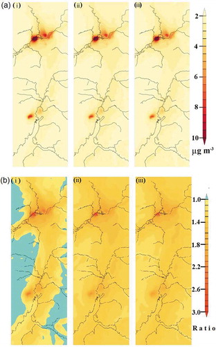
Figure 5 shows post-correction spatial plots of AM for all three schemes. Pollutant concentrations are quite similar among schemes, and below 8 μg m⁻³ except for a small area (4–5 grid cells) just west of Terrace. Here, modeled concentrations attain maximum values of 18.3, 12.7 and 29.2 μg m⁻³ for SIMPLE, POWER and DEG_2, respectively, as against 7.3 μg m⁻³ in the original output. Apart from SIMPLE for which bias-corrected results in less concentrations over the ridges compared to the original model output (0.8–1.0 ratio), corrected values are mainly 1–2 times of the original output, and up to 3 times for the greatest concentrations. Highest post-correction PM_2.5 levels for the Terrace area are consistent with expectations for urban settings, but there is also a small area of comparable levels around the Haul Road station, near the coastal outlet. This area is an industrial zone where particulate emissions from an existing smelter and allied services are probably a major contributor. Sideward spread of stack emissions is restricted by valley walls to the west of the industrial hub; hence, a localized area that is closer to limit values than the rest of the Kitimat area. Away from Terrace and Kitimat areas, modeled AM is less than 3 μg m⁻³.

Figure 5. Spatial plot of bias-corrected annual mean PM_2.5 concentrations (a), and ratio of bias-corrected concentrations to those of the original model output (b) for (i) SIMPLE (ii) POWER and (iii) DEG_2

Estimation of background concentrations

Based on the close fit between bias-corrected output with observation for annual air quality management metric, background PM_2.5 concentrations in the valley can be estimated. Background concentrations are pollutant levels in the absence of local anthropogenic emissions and represent the sum of concentrations arising from natural processes and those transported into an airshed from afar (McKendry 2006). Ideally, long-term pollutant monitoring at a pristine site would provide background concentrations, but in its absence in the valley, and based on local knowledge, an unmonitored, uninhabited position in the modeling grid, distant from major emission areas is used. This position (Figure 6) that is currently devoid of anthropogenic PM_2.5 sources and thus representative of background conditions, is about 30 km from Terrace and Kitimat.

Figure 6. Centerline profile of bias-corrected annual mean concentrations

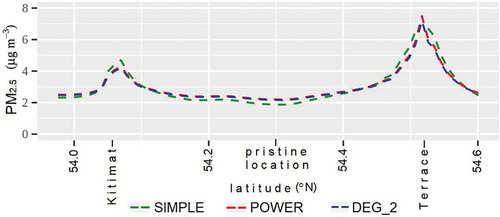
Figure 6 indicates that the mean annual background concentration of PM_2.5 for the valley is 2.0–2.3 μg m⁻³. The annual mean plots in Figure 5 also hint at this range, but it is worth mentioning that pristine environments are not confined to within the valley alone. The mountain slopes and high-altitude areas are also wildernesses. On the western mountain ridges that are exposed to Pacific air masses, occur minimum concentrations of 1.0, 1.8 and 1.4 μg m⁻³ for SIMPLE, POWER and DEG_2 schemes, respectively. Given the role of transcontinental transport in redistributing atmospheric aerosol and the relative isolation of the TKV from significant anthropogenic North American sources, these minimums can be regarded as background concentrations affecting this part of the North American west coast. These concentrations would result from emissions over the ocean including sea salt (although this source would have a larger impact area like the valley bottom that are within the MBL), contributions from Eurasian sources undergoing transpacific transport, and wind-blown dust within the domain. Episodic particulate transport due to large-scale, natural, seasonal emergencies might influence observed background concentrations. For example, the summer of 2017 was one of the worst forest fire seasons in the BC Interior in recent history. Although the northwest BC coast is often spared the heaviest smoke in such events (BCMOE 2017; Elliott, Henderson, and Wan 2013) due to predominantly westerly atmospheric circulation, increased dust and intermittent advection of particulate matter from slash burns in the dry months possibly contribute to highest background levels in the summer season (Table 7). Emissions from wildfires are not included in the model emission inventory.

Table 7. Annual and seasonal background PM_2.5 levels in the TKV with the various bias-correction formulas

Bias correction	Spring	Summer	Autumn	Winter	Annual
SIMPLE	2.10	2.22	1.78	1.68	1.95
DEG2	2.32	2.41	2.10	2.03	2.21
POWER	2.35	2.44	2.13	2.07	2.25

Discussion

The application of linear regression models to CMAQ model output improved representation of ambient PM_2.5 over the TKV. The final products from the mathematical formulations were generally comparable, with slightly better agreement of modeled and station data from a correction based on the power transform of the original model output. Improvements are remarkable since corrections were not site-specific, rather, emanated from training with data from an urban location. The POWER formula, for example, reduced autumn NMSE from 1.9 to 1.2 at Haul road, and from 1.1 to 0.6 at Riverlodge, representing 37% and 45% decreases respectively from the original model outputs. Djalalova, Delle Monache, and Wilczak (2015) reported 50–75% reduction in absolute errors with a Kalman filter–analog combination over the contiguous USA. Nonetheless, it is difficult to compare the present study with error reduction demonstrations elsewhere because apart from dissimilarities in geographical settings, there are differences in statistical measures employed, including averaging periods, data collation methods and observation network densities. We reiterate that PM_2.5 modeling bias-correction literature has mainly been on operational forecasting for much larger geographical areas and with higher ambient concentrations than in the TKV. In China where ambient particulate measurements are much higher, Lyu, Zhang, and Hu (2017) found that for a suite of 12-km forecast correction techniques, reductions in normalized mean errors were in the ranges of 7.4–19% for 1-day lead time. Bias corrections in this study applied retrospectively to simulations on a 1-km horizontal grid, thus demonstrate the efficacy of quantile-based statistical techniques to improve the usability of chemical transport model outputs over complex terrain with sparse monitoring.

Degraded springtime FAC2 and NMSE, alongside improved statistics for autumn and winter seasons following bias corrections, suggested error compensations that were beneficial to modeling accuracy for periods of peak ambient PM_2.5. Further, there was a remarkable improvement in the representation of compliance metrics for bias-corrected ambient levels. Since the time order of hourly concentrations was not critical to determining whether the TKV complies with existing PM_2.5 standards, the approach of using regression models that are based on quantile-means for bias correction is valuable to airshed management. Specifically, corrections reduced large biases for the percentile-based daily metric to an average error of 10%. A comparable effect was also obtained for the annual metric. The significance of improved agreement of simulations with observations is more confidence in base PM_2.5 contour maps that are generated since regulatory compliance purposes of continuous monitors suffer from poor spatial coverage. For epidemiological studies on community health effects of particulate matter, such spatial representations are indispensable. Because the frequency of post-correction negative biases was slightly less for the daily metric than the annual metric, the use of refined outputs for health assessment could be more pessimistic of long-term (chronic) than short-term (acute) exposures.

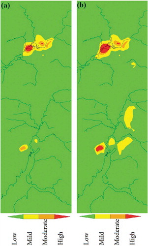
This view follows from transforming ambient PM_2.5 levels into an exposure risk ranking (Figure 7) according to thresholds that are enunciated by CCME (2012) and applicable to the province of British Columbia. Quite suggestive is that a small area just west of Terrace may be in violation of provincial air quality objectives. At this stage, it is not certain the number of persons that may be impacted if borne out in reality, since this zone is outside the urban core. Indeed, one shortcoming is that our assessment does not account for effective exposure, which depends on the duration and frequency of outdoor activity by individuals. Nonetheless, the evaluation hints at the possibility of an ongoing problem. Whereas collecting ambient data and public education on local air quality are appropriate for all areas, additional surveillance and analysis of trends can assist with confirming the actual source of the higher levels of PM_2.5. This may warrant ground-truthing over several months, to rule out the need for costly regulatory measures that may not be required in the present.

Figure 7. Color-coded classification of modeled PM_2.5 ambient exposure risk from POWER scheme using thresholds in Figure 4a. (a) annual metric; (b) daily metric

Background pollutant concentrations were determined from bias-corrected values within the model domain, rather than using CMAQ boundary conditions. This was necessary because PM_2.5 constituents are not summed in the CMAQ boundary concentration file. The estimated mean annual background concentration of PM_2.5 over the TKV was 2.0–2.3 μg m⁻³ which is comparable to 2 μg m⁻³ suggested by McKendry (2006) for the entire BC province; and 2.5 μg m⁻³ reported by Vingarzan (2007) for all of Canada. This is also within the range of 1–4 µg m⁻³ estimated for the western United States (Environmental Protection Agency 1996) which like the TKV, is affected by trans-Pacific aerosol transport. It needs mentioning that these works pertain to large geographical areas encompassing diverse physical environments and eco-climatic zones. The lower limit of the annual background mean value from the present study is 0.2 µg m⁻³ higher than the lower end of 1.8–2.5 µg m⁻³ range calculated for locations in the BC Interior (Veira et al. 2013). Although the coastal setting of the TKV provides for exposure to both maritime and continental air masses, the valley possibly does not have higher background levels than areas further inland. Perhaps, differences in estimates could be more due to the estimation methods adopted by the various authors. For example, Veira et al. (2013) was for locations in small cities and was based on analysis of wind sectors, for which trajectories were assumed to have passed over negligible upwind sources of anthropogenic emissions. PM_2.5 background concentration in our study is within the range 1.7–3.8 μg m⁻³ from a study that was based on monitoring data of six remote rural locations in Alberta (Cheng et al. 2000). In fact, dispersion modeling with the CALPUFF model in the TKV (ESSA Technologies, Risk Sciences International, and Trinity Consultants 2015) used background PM_2.5 levels ranging from 2.2 to 3.6 μg m⁻³ for post-processing of output concentrations at individual receptor locations. These comparisons allude to the usefulness of bias-corrected outputs of a chemical transport model (CTM) over pristine areas to estimate background PM_2.5 concentrations.

The desired goal of air quality objectives in British Columbia, especially within residential areas is that PM_2.5 concentrations do not exceed 8 μg m⁻³ annual average. The mean annual background PM_2.5 concentrations of 2–2.3 μg m⁻³ in our study translates to 25–30% of the provincial limit. It is reassuring that 2017 ambient concentrations for a vast portion of the valley are close to this level, implying that a “business as usual” economic activity in the area should sustain good air quality. Because aerial exceedance of the provincial annual metric is also small, isolated issues can be dealt with as they arise. However, in the event that proposed industries become operational, or work camps are built in confined neighborhoods, the adoption of local target limits for ambient PM_2.5 will be beneficial. Specifically, and irrespective of targets that may be advanced, the Terrace area, where topographical and meteorological conditions seem less favorable to dispersion of pollutants, and where some of the additional industrial workforce could reside, should be prioritized for particulate emission abatement. Overall, it is important that airshed plans for the TKV, especially for PM_2.5, recognize that although anthropogenic emissions are low for the most part at present, the natural background constitutes a portion of the ambient level that is not amenable to control.

Summary and conclusion

Chemical transport models can have large biases and errors when simulating pollutant concentrations. To improve PM_2.5 modeling over complex terrain so that gridded fields of pollutant levels can be used for exposure assessments, we developed mathematical formulae that utilized relationships between quantile mean concentrations of model outputs and observational data. They were applied to CMAQ model simulation of PM_2.5 for 2017 over the Terrace–Kitimat Valley of northwestern British Columbia, Canada. Numerical adjustment of hourly concentrations for all grid cells within the domain was achieved. The final products were found to enhance the representation of ambient levels at existing monitoring stations when evaluated with conventional statistical measures. Better agreement of refined outputs with observed compliance metrics ensured greater confidence for use of the resulting gridded outputs to estimate concentrations at locations without monitors. The fact that pristine conditions dominate the modeling domain was exploited to derive annual background PM_2.5 concentrations, which was estimated to be 2.0–2.3 μg m-³. To our knowledge, this is the first study to calculate background PM_2.5 concentrations over northern BC coastlands using bias corrected CMAQ output.

This work is significant in a number of ways. Methodologically, it provides support for use of simple, comprehensible techniques to improve CTM outputs that are discrepant from observational data due to errors in meteorological and emission inputs. An important contribution from a regulatory perspective was adjusting simulated concentrations and implementing the corrections throughout the TKV modeling grid. The TKV, like much of northern BC, is sparsely monitored and the realization of more reliable PM_2.5 spatial distribution offers a suitable proxy for community exposures. Second, refined model outputs supplement information for directing actions to sustain good air quality. While routine monitoring and reporting from existing particulate measurement stations are appropriate under present PM_2.5 levels, isolated areas of elevated concentrations can benefit from extended monitoring to identify the major causes. Finally, estimated background concentrations in our study constitute a portion of air quality objectives that should be considered in setting voluntary targets for ambient PM_2.5 in the area. Such reckoning is important since more industrial facilities in the TKV may lead to significant particulate emissions.

Acknowledgment

This study was supported by the Natural Sciences and Engineering Research Council of Canada Discovery Grant RGPIN-2017-05784 to Peter Jackson. The authors acknowledge the support of high-performance computing resources from the University of Northern British Columbia for pollutant modeling. We appreciate the comments of four anonymous reviewers whose suggestions improved this manuscript.

Supplementary material

Supplemental data for this article can be accessed on the publisher’s website.

Disclosure statement

The authors declare that they have no known competing financial interests or personal relationships that influence the work reported in this paper.

Additional information

Funding

This work was supported by the Natural Sciences and Engineering Research Council of Canada [RGPIN-2017-05784].

Notes on contributors

Chibuike Onwukwe

Chibuike Onwukwe is an air quality meteorologist and modeler whose research is majorly on quantifying the environmental effects of industrial emissions in remote communities.

Peter L. Jackson

Peter L. Jackson is a mesoscale meteorologist whose research mostly concerns the interaction between the atmosphere and complex terrain (i.e. in mountains and along coastlines) and how this affects wind, precipitation, climate and air quality.

References

- Appel, K. W., S. Napelenok, C. Hogrefe, G. Pouliot, K. M. Foley, S. J. Roselle, J. E. Pleim, J. Bash, H. O. T. Pye, N. Heath, et al. 2018. Overview and evaluation of the community multiscale air quality (CMAQ) modeling system version 5.2. In Air pollution modeling and its application XXV, ed. C. Mensink and G. Kallos, 69–73. Cham: Springer. doi:10.1007/978-3-319-57645-9_11.
- Atkinson, R. W., I. C. Mills, H. A. Walton, and R. H. Anderson. 2015. Fine particle components and health—a systematic review and meta-analysis of epidemiological time series studies of daily mortality and hospital admissions. J. Expo. Sci. Environ. Epidemiol. 25:208–14. doi:10.1038/jes.2014.63.
- BCMOE (British Columbia Ministry of Environment and Climate Strategy). 2020. Provincial air quality objective for PM2.5. https://www2.gov.bc.ca/gov/content/environment/air-land-water/air/air-quality-management/regulatory-framework/objectives-standards/pm2-5.
- BCMOE (British Columbia Ministry of Environment and Climate Strategy). 2017. Coastal zone air report (2015–2017). https://www2.gov.bc.ca/assets/gov/environment/air-land-water/air/reports-pub/air-zone-reports/2015-2017/coastal_air_zone_report_2015-2017.pdf.
- Borrego, C., A. Monteiro, M. T. Pay, I. Ribeiro, A. I. Miranda, S. Basart, and J. M. Baldasano. 2011. How bias-correction can improve air quality forecasts over Portugal. Atmos. Environ. 45:6629–41. doi:10.1016/j.atmosenv.2011.09.006.
- CCME (Canadian Council of Ministers of the Environment). 2012. Guidance document on air zone management. https://www.ccme.ca/files/Resources/air/aqms/pn_1481_gdazm_e.pdf.
- Chang, J., and S. Hanna. 2004. Air quality model performance evaluation. Meteorol. Atmos. Phys. 87:167–96. doi:10.1007/s00703-003-0070-7.
- Cheng, L., H. S. Sandhu, R. P. Angle, K. M. McDonald, and R. H. Myrick. 2000. Rural particulate matter in Alberta, Canada. Atmos. Environ. 34:3365–72. doi:10.1016/S1352-2310(00)00123-0.
- Crouse, D. L., P. A. Peters, A. van Donkelaar, M. S. Goldberg, P. J. Villeneuve, O. Brion, S. Khan, D. O. Atari, M. Jerrett, C. A. Pope, et al. 2012. Risk of nonaccidental and cardiovascular mortality in relation to long-term exposure to low concentrations of fine particulate matter: A Canadian national-level cohort study. Environ. Health Perspect. 120:708–14. doi:10.1289/ehp.1104049.
- District of Kitimat. 2019. Current major projects. https://www.kitimat.ca/en/business-and-development/current-major-projects.aspx.
- Djalalova, I., L. Delle Monache, and J. Wilczak. 2015. PM2.5 analog forecast and kalman filter post-processing for the community multiscale air quality (CMAQ) model. Atmos. Environ. 108:76–87. doi:10.1016/j.atmosenv.2015.02.021.
- Elliott, C. T., S. B. Henderson, and V. Wan. 2013. Time series analysis of fine particulate matter and asthma reliever dispensations in populations affected by forest fires. Environ. Health 12:11. doi:10.1186/1476-069X-12-11.
- Emery, C., Z. Liu, A. G. Russell, M. T. Odman, G. Yarwood, and N. Kumar. 2017. Recommendations on statistics and benchmarks to assess photochemical model performance. J. Air Waste Manage. 67:582–98. doi:10.1080/10962247.2016.1265027.
- Environment and Climate Change Canada. 2019. Canadian climate normals 1981-2010 station data. http://climate.weather.gc.ca/climate_normals/results_1981_2010_e.html?stnID=402&autofwd=1.
- Environmental Appeal Board. 2015. Decisions: Emily Toews; Elisabeth Stannus v. Director, Environmental Management Act (Rio Tinto Alcan Inc., Third Party), 1–2, 58–84. http://www.eab.gov.bc.ca/ema/2013ema007g_010g_corrigendum_2.pdf.
- Environmental Protection Agency. 1996. Air quality criteria for particulate matter. Report nos EPA/600/P-95/001aF-cF. 3v, National Center for Environmental Assessment-RTP Office, Research Triangle Park, NC. https://nepis.epa.gov/Exe/ZyPDF.cgi/20008MAJ.PDF?Dockey=20008MAJ.PDF.
- ESSA Technologies, Risk Sciences International, and Trinity Consultants. 2015. PM2.5 supplement to the Kitimat airshed emissions effects assessment. Prepared for BC Ministry of Environment, Smithers, BC, 19. https://www2.gov.bc.ca/assets/gov/environment/air-land-water/air/reports-pub/2015-03-31_essa-pm2-5_suppl-kaeea.pdf.
- Ghim, Y. S., Y.-S. Chang, and K. Jung. 2015. Temporal and spatial variations in fine and coarse particles in Seoul, Korea. Aerosol Air Qual. Res. 15:842–52. doi:10.4209/aaqr.2013.12.0362.
- Huang, J. P., J. McQueen, J. Wilczak, I. Djalalova, I. Stajner, P. Shafran, D. Allured, P. Lee, L. Pan, D. Tong, et al. 2017. Improving NOAA NAQFC PM2.5 predictions with a bias correction approach. Weather Forecast. 32:407–21. doi:10.1175/WAF-D-16-0118.1.
- Kang, D., R. Mathur, and S. T. Rao. 2010. Assessment of bias-adjusted PM2.5 air quality forecasts over the continental United States during 2007. Geosci. Model. Dev. 2:309–20. doi:10.5194/gmd-3-309-2010.
- Krudysz, M., K. Moore, M. Geller, C. Sioutas, and J. Froines. 2009. Intra-community spatial variability of particulate matter size distributions in Southern California/Los Angeles. Atmos. Chem. Phys. 9:1061–75. doi:10.5194/acp-9-1061-2009.
- Li, P. 2005. Box-Cox Transformations: An Overview. Department of Statistics, University of Connecticut. https://www.ime.usp.br/~abe/lista/pdfm9cJKUmFZp.pdf.
- Lyu, B., Y. Zhang, and Y. Hu. 2017. Improving PM2.5 air quality model forecasts in China using a bias-correction framework. Atmosphere 8:147. doi:10.3390/atmos8080147.
- McKendry, I. G. 2006. Background concentrations of PM2.5 and ozone in British Columbia, Canada. Vancouver: University of British Columbia. http://citeseerx.ist.psu.edu/viewdoc/download?doi=10.1.1.510.4465&rep=rep1&type=pdf.
- Neal, L. S., P. Agnew, S. Moseley, C. Ordonez, N. H. Savage, and M. Tilbee. 2014. Application of a statistical post-processing technique to a gridded, operational, air quality forecast. Atmos. Environ. 98:385–93. doi:10.1016/j.atmosenv.2014.09.004.
- Onwukwe, C., and P. Jackson. 2020a. Evaluation of CMAQ modeling sensitivity to planetary boundary layer parameterizations for gaseous and particulate pollutants over a fjord valley. Atmos. Environ. 233:117607. doi:10.1016/j.atmosenv.2020.117607.
- Onwukwe, C., and P. Jackson. 2020b. Meteorological downscaling with WRF model, version 4.0, and comparative evaluation of planetary boundary layer schemes over a complex coastal airshed. J. Appl. Meteor. Climatol. 59:1295–319. doi:10.1175/JAMC-D-19-0212.1.
- Pinto, J. P., A. S. Lefohn, and D. S. Shadwick. 2004. Spatial variability of PM2.5 in urban areas in the United States. J. Air Waste Manage. 54:440–49. doi:10.1080/10473289.2004.10470919.
- Porter, P. S., S. T. Rao, C. Hogrefe, E. Gego, and R. Mathur. 2015. Methods for reducing biases and errors in regional photochemical model outputs for use in emission reduction and exposure assessments. Atmos. Environ. 112:178–88. doi:10.1016/j.atmosenv.2015.04.039.
- Skamarock, W. C., J. B. Klemp, J. Dudhia, D. O. Gill, Z. Liu, J. Berner, W. Wang, J. G. Powers, M. G. Duda, D. M. Barker, et al. 2019. A description of the advanced research WRF version 4. NCAR Tech. Note NCAR/TN-556+STR, 145. doi: 10.5065/1dfh-6p97.
- Solazzo, E., and S. Galmarini. 2016. Error apportionment for atmospheric chemistry-transport models – A new approach to model evaluation. Atmos. Chem. Phys. 16:6263–83. doi:10.5194/acp-16-6263-2016.
- Statistics Canada. 2018. Census profile, 2016 census. http://www12.statcan.gc.ca/census-recensement/index-eng.cfm?GEOCODE=59#keystats.
- UNC (University of North Carolina). 2009. Sparse matrix operator Kernel emissions. https://www.cmascenter.org/smoke/documentation/2.6/html/.
- Veira, A., P. L. Jackson, B. Ainslie, and D. Fudge. 2013. Assessment of background particulate matter concentrations in small cities and rural locations—Prince George, Canada. J. Air Waste Manage. 63:773–87. doi:10.1080/10962247.2013.789091.
- Vingarzan, R. 2007. Ambient particulate matter concentrations in Canada and background Levels. Vancouver: Environment Canada, Meteorological Services Branch. http://publications.gc.ca/collections/collection_2007/ec/En56-215-2007E.pdf.
- WHO. 2016. Ambient air pollution: A global assessment of exposure and burden of disease. Geneva: World Health Organization. https://www.who.int/phe/publications/air-pollution-global-assessment/en/.
- Wilson, J. G., S. Kingham, J. Pearce, and A. P. Sturman. 2005. A review of of intraurban variations in particulate air pollution: Implications for epidemiological research. Atmos. Environ. 39:6444–62. doi:10.1016/j.atmosenv.2005.07.030.
- Zurbenko, I. G., and M. Sun. 2017. Applying Kolmogorov-Zurbenko adaptive R-software. Int. J. Stat. Probab. 6:110. doi:10.5539/ijsp.v6n5p110.