Evaluation of OSPM against air quality measurements in Brazil – the case study of Fortaleza, Ceará

ABSTRACT

The contribution of vehicle emissions to air pollution is considered a large environmental and health problem in big Brazilian cities caused, among other factors, by slow renewal of the old vehicle fleet. Brazilian studies usually only consider traffic-related issues in transportation analysis, with minor assessments of emissions and close to non-existent assessment of air quality. On this background, this research aimed to calibrate and evaluate the Operational Street Pollution Model (OSPM®) to Brazilian conditions by implementing Brazilian emission factors. The urban background concentrations were modeled with the Urban Background Model (UBM) as part of the air quality system (THOR–AirPAS). In this case, we used meteorological data from a ground meteorological station outside Fortaleza processed by meteorological pre-processor and regional background concentrations from the Integrated Forecast System (IFS) as input to UBM. New air quality measurements were collected in busy streets of the city of Fortaleza during the year of 2017. The study collected samples of daily NO₂ and PM₁₀ concentrations to evaluate OSPM daily estimations. In addition, a transportation travel demand model (TRANUS) has been calibrated to the case study area with observed traffic data collected, in order to provide Annual Average Daily Traffic (AADT) as inputs to OSPM®. Two sets of emission factors were evaluated. Official Brazilian emission factors were applied to OSPM®, as well as adjusted emission factors derived in the project based on calibration that were higher than the official emission factors. Data showed that concentrations are significantly influenced by meteorological factors (such as temperature, wind speeds, wind directions), and especially precipitation for PM₁₀ concentrations. OSPM® simulated results showed concentration levels and patterns close to air quality measurements with default emission factors and calibrated emission for UBM but large underestimations if official emissions were used for both UBM and OSPM.

Implications: Busy urban streets in Brazilian cities with intense flow of diesel vehicles (such as buses and trucks) can significantly increase air pollution, especially for NO₂ and PM₁₀. With OSPM calibrated and evaluated to Brazilian conditions, the model system can be used by authorities to assess the impact of policy measures, such as vehicle access restrictions in Low Emission Zones, in order to consider not only traffic related issues, but also air pollution due to mobile sources with outdated emission technologies.

Introduction

According to the latest air quality database, 97% of cities in low and middle income countries with more than 100,000 inhabitants do not meet World Health Organization (WHO) air quality guidelines (WHO, 2018).

In Brazil, in the city of Rio de Janeiro, for example, 77% of the population is exposed to levels above the WHO guidelines (Coelho, 2006). Thus, when planning for improvements in urban mobility, not only indicators that result in improved traffic related issues should be observed, but also those that impact on human health, especially those related to air quality. In addition, Heavy Duty Vehicles (HDVs) make up only 5% of the vehicle fleet in Sao Paulo city but have been found to contribute 40% of benzene and 47% of black carbon concentrations, showing the large contribution from HDVs in urban areas (Brito et al. 2018). In newly industrialized countries, such as Brazil, traffic-related NO₂ and PM₁₀ air pollution is particularly high, due to old vehicle fleet technology with high emission factors from inefficient engines and control technologies (CETESB, 2017a).

Air pollution is a major cause of diseases. It is estimated that at least 3% of cardiopulmonary and 5% of lung cancer deaths are attributable to PM globally (WHO 2013). NO₂ has been associated with adverse effects on hospital admissions for various diagnoses, decrements in measures of lung function and lung function growth, increases in respiratory symptoms, asthma prevalence and incidence, cancer incidence, adverse birth outcomes, and mortality (US EPA, 2013; WHO, 2013). The most recent study on the Global Burden of Disease estimates that 7.5% of premature deaths globally were attributable to ambient air pollution in 2016. In the same year, 27.5% of deaths due to Lower Respiratory Tract Infections and 26.8% of deaths due to Chronic Obstructive Pulmonary Diseases were linked to air pollution (Li and Mallat 2018). All of these negative effects lead to an increase in the socioeconomic costs due to health impacts while also influencing quality of life (Darcin 2014; Vienneau et al. 2015).

To estimate air pollution concentrations of NO₂ and PM₁₀ in street levels, this research aims to calibrate and evaluate the Operational Street Pollution Model (OSPM) to Brazilian conditions with Fortaleza as case study to develop a model system for decision-support of traffic-related measures such as for example Low Emission Zones, which are still not implemented in Brazil (ICCT, 2019). Previous studies were successful in modeling air quality in Brazil (Andrade et al. 2015; Krecl et al. 2015, 2019, 2018, 2016). However, these previous approaches aimed to study regional concentrations or street concentrations with only one street observed, with different air pollutants. In addition, previous studies observe the southern/south region of Brazil only. The new approach presented in this study combines travel demand modeling and air quality modeling, and is the first of its kind in Brazil. The study area is Fortaleza, Ceará, Brazil (03° 43ʹ 02ʹ’ south latitude and 38° 32ʹ 35ʹ’ west longitude, Northern Region), which suffers from high vehicle density, thus being highly affected by traffic-related air pollution. Fortaleza is a typical big Brazilian city, which can represent traffic-related air pollution in general in developed cities in the country. OSPM presents a more detailed mechanism for physical behavior in roads with a presence of tunnels and urban canyons when compared to other street air pollution models (Martins, Fortes, and Lessa 2015), which is specifically accurate to observe in this study. In addition, OSPM is the final modeling step in air quality modeling system THOR-AirPAS, a sophisticated modeling system which integrates regional background concentrations (in this study performed with Integrated Forecast System, IFS), urban background concentrations (embedded in THOR-AirPAS system, Urban Background Model, UBM) and street levels air pollution concentrations (last step, OSPM) (DCE 2014). OSPM is capable of disaggregate different types of vehicles, several different pollutants (some air pollution models are not capable of estimating NO₂ and PM₁₀)m and different scenario configurations (Berkowicz et al. 1997; Berkowicz, Olesen, and Jensen 2003).

Air quality measurements with passive samplers for NO₂ and active samplers for PM₁₀ in selected streets were carried out for this research for air quality assessment and model evaluation as there are few air quality monitoring stations in Brazilian cities with reliable data.

All required input data for the OSPM) was generated using different tools and models, and OSPM was calibrated and evaluated against the air quality measurements. The overall methodology for this study, results, discussion, and conclusion are presented as follows.

Methods

Overall methodology

Figure 1 shows the methodology applied in this research to evaluate OSPM modeled air pollutant concentrations against observed measurements at street levels.

Figure 1. Flowchart of methodology to evaluate OSPM air pollutant concentration estimations against observed concentrations at street level, Fortaleza, Ceará–Brazil

OSPM is used to calculate street concentrations for comparison and evaluation against collected air quality measurements at selected streets. OSPM requires inputs concerning traffic data and street geometry, vehicle emissions, urban background concentrations, and meteorology. Urban background concentrations are calculated with UBM. UBM estimate concentrations at a receptor by numerical integration of contribution from each of the individual area sources along each actual wind direction path upwind to 30 km from the receptor, where the rural background is used as boundary condition (in this case, results from the IFS model). The horizontal diffusion is assumed to follow a Gaussian function. UBM is set up to calculate the following pollutants: NO_x (nitrogen oxides), NO₂ (nitrogen dioxide), O₃ (ozone), SO₂ (sulfur dioxide), CO (carbon monoxide), TSP (total suspended particulate matter), PM₁₀ (particles less than 10 μm in diameter), and PM_2.5 (particles less than 2.5 μm in diameter) (Danish Center for Environment and Energy 2014). UBM requires inputs on gridded emissions, regional background concentrations, and meteorology. In this study, the regional background concentrations were estimated using IFS instead of Danish Eulerian Hemispheric Model (DEHM) since the latter only covers the Northern Hemisphere (Cristensen 1997). IFS is capable of estimating global Ozone (O₃), Nitrogen Monoxide (NO), Nitrogen Dioxide (NO₂), Carbon Monoxide (CO), and disaggregated particles, such as seasalt, dust, hydrophilic organic matter, hydrophobic organic matter, hydrophilic black carbon, and hydrophobic black carbon. IFS operates with a spatial resolution of about 80 km and three-hourly time resolution (Flemming et al. 2015).

Meteorological data for UBM and OSPM is based on processed meteorological data from a ground meteorological station outside Fortaleza using a meteorological pre-processor. THOR-AirPAS is an air pollution assessment system that has a user interface to OSPM and UBM to ease interaction with input data, air quality models, and output data (Jensen et al. 2014).

In the following, the case study area and the air quality measurement campaign are described, and the models UBM and OSPM are described in brief together with the generation of model input data.

Case study area of Fortaleza

Fortaleza is the capital of Ceará State and the fifth biggest city of Brazil, located in Northeastern Brazil, with a population of approx. 2.6 million inhabitants in 2017 (Instituto Brasileiro de Geografia e Estatística [IBGE], 2018). Fortaleza is a tourist city. In addition, it is one of the main destinations for agricultural products from municipalities in Ceará and other states and also supports these areas with public and private services. The total land area of Fortaleza is 315 km², which includes 119 districts in five regions throughout the city (Fortaleza 2018).

Fortaleza has a typical tropical climate, with a wet and dry season, high temperatures, and high relative humidity throughout the year. The annual mean precipitation is approximately 1,448 mm, and the annual mean temperature (T) is 26.3 °C (Funceme 2018). In general, Fortaleza is a typical, prosperous coastal city in Brazil. The air quality in this economically developed city is influenced by vehicle traffic, especially due to an old vehicle fleet (Lopes et al. 2018).

Air quality measurements

There were no permanent air quality monitoring stations in Fortaleza at the time of this study, ecept for one monitoring station in the city of Pecém (metropolitan region of Fortaleza), which does not provide reliable data to assess air pollution at street levels of the case study area (SEMACE 2016). Therefore, a methodology was developed to collect measurements of NO₂ and PM₁₀. Air pollutants data collection has been carried out in the case study area of Fortaleza on locations with high vehicle flow density and high population density. Locations were also chosen to reflect differences in heavy-duty traffic and urban canyon characteristics (different ratios of building height/street width). Passive samplers for NO₂ concentrations were developed especially for this research based on Palmes and Lindenboom (1979) method, which transfers the tested NO₂ gas through a tube of known dimensions using Fick’s First law, adapting the NO₂ sampler with a device suitable for data collection in public lighting poles, in order to passively absorb NO₂ in street levels. Cases were constructed for use in street lighting poles (with a structure to resist rain, wind, and small impacts), and samplers data collected NO₂ concentrations in street levels, observing data during 24 hours. The values have been obtained by means of spectrophotometry and chromatography techniques.

Active measurements of PM₁₀ concentrations have been performed based on gravimetric analysis to calculate the concentrations. The equipment used was an Ecotech HiVol 3000 (High Volume Particulate Sampler). PM₁₀ mass is accumulated on a filtering membrane, and filters were weighted before and after the data collection, through 24 hours, and divided by the total sampled volume, thereby reaching the PM concentrations (24 hours data collections for PM₁₀, in µg/m³).

The calibration and quality assurance (QA) of both data collection methods have been reported by Ribeiro et al. (2018) and Alcântara et al. (2019). Air quality measurements were collected in two campaigns to assess the unique seasonal variation in Northern Brazil which has a rainy season (March to May) and a dry season (rest of the year). Daily concentrations of NO₂ and PM₁₀ were measured for 24 hours in each day (usually 08:00 a.m. to 07:00 a.m. the following day, due to operational reasons).

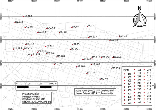
First campaign was carried out between May 8 and June 1, and the second campaign from November 19 to December 3, 2017. Due to equipment availability, time for data collection, and safety reasons, we had to data collect NO₂ and PM₁₀ in different times and locations. In the first and second campaigns, data collection has been successfully carried out for all data collection points with the exception of NO₂ in the first campaign where two samplers missed out for unknown reasons. NO₂ were collected with passive samplers in both campaigns at 20 locations (201 to 220 in Figure 3), and PM₁₀ were collected with an active method during both campaigns at 12 locations (101 to 112 in Figure 3). The sampling height was approx. 2.5 m to avoid destruction or other operational problems. Figure 2 shows the location of the case study area and Figure 3 displays the location of data collection points for air quality measurements within the highlighted studied area, and the concentrations observed in second campaign just for sake of illustration (second campaign chosen due to two missing NO₂ observations in first campaign).

Figure 2. Zoom in on location of study area: Brazil, Ceará, Fortaleza, case study area

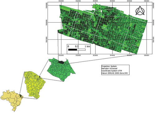
Figure 3. Active (PM₁₀) and passive (NO₂) data collection points within highlighted studied area presented in Figure 2. PM₁₀ data collection points have the format 1xx and NO₂ data collection points 2xx. Second campaign concentrations are shown after the number of the collection point

Urban background model (UBM)

Urban background concentrations have been calculated with the Urban Background Model (UBM) (Berkowicz 2000b; Brandt et al. 2003) as part of the THOR-AirPAS system (Jensen et al. 2014). Concentrations are estimated by numerical integration contributions from each of the individual area sources along each actual wind direction path upwind to 30 km from the receptor point, where the regional background concentrations are used as boundary. The horizontal diffusion is assumed to follow a Gaussian function. The step size is 50 m in the numerical integration both along the wind direction and perpendicular to the wind direction, where horizontal diffusion is taken into account. In the present study, a vehicle emissions database with a spatial resolution of 1 km x 1 km has been developed based on traffic data on a road network and vehicle emission factors as input for UBM. The concentrations of NO₂ and PM₁₀ are calculated with a 1 hour time resolution.

Operational street pollution model (OSPM)

Street level air pollutant concentrations have been estimated with the OSPM (Berkowicz 2000a; Berkowicz et al. 2008; Kakosimos et al. 2010; Ketzel et al. 2012). OSPM is a semi-empirical atmospheric dispersion model for simulating the dispersion of air pollutants near streets with different building geometry, including open or half-open streets and so-called street canyons. Concentrations of traffic-emitted pollution are calculated using a combination of a plume model for the direct contribution and a box model for the recirculating part of the pollutants in the street. NO₂ concentrations are calculated taking into account NO-NO₂-O₃ chemistry and pollutants residence time in streets. The model is designed to work with input and output in form of one-hour averages. OSPM is capable of estimation of various pollutants provided emission data is available. In the present study, hourly NO₂ and PM₁₀ concentrations were calculated and aggregated by day (24 hours), in order to compare with observed concentrations collected in the streets.

OSPM requires input on traffic and street configuration data, vehicle emissions, urban background concentrations, and meteorological data. The collection and generation of input data are explained in what follows.

Traffic and street configuration data for OSPM

The input data for the OSPM on traffic data and street configurations for the selected urban streets where air quality measurements were carried out are generated using the AirGIS system based on Geographic Information System (GIS) maps of a road network with traffic data, building foot-prints with building heights and calculation points (Jensen et al. 2001, 2017; Ketzel et al. 2011). Street configurations include, for example, street orientation, width of street, building heights in different wind sectors, and so on.

Traffic data for OSPM at air quality measurement locations

Traffic data has been collected with Split Cycle Time and Offset Optimization Technique (SCOOT) system. SCOOT uses inductive loop-type sensors and video cameras to monitor street traffic and to calculate the Annual Average Daily Traffic (AADT), data collected by Controle de Tráfego em Área de Fortaleza (CTAFOR) (Traffic Control in Fortaleza Area) (CTAFOR, 2015).

Traffic data has been collected for the same locations as the air quality measurements points as part of traffic data input to OSPM. SCOOT system was developed to perform traffic control in real time, requiring constant data between field controllers and a central computer. This system allows monitoring the operation of all traffic lights: controllers, detectors, focus groups, and lamps (Loureiro, Leandro, and Oliveira 2002). This system works in real time with traffic signal programming determined dynamically by dedicated systems, based on traffic data collected by field inductive loop-type sensors in the streets (Oliveira 1997). Monitored traffic data with a time resolution of 15 minutes was expanded to a whole day by SCOOT system, in order to calculate the AADT used as input for OSPM (Alves 2014). Diurnal variations in this study considered SCOOT traffic data and real traffic data collection to validate SCOOT outputs (e.g., vehicle types, speed, flow). OSPM also requires input on vehicle distribution that was provided by SCOOT and traffic counts. Furthermore, OSPM requires input on the temporal variation of traffic in order to estimate hourly values. Here, standard diurnal profiles for the different vehicle categories were used.

Travel demand modeling of road network

In order to code and calibrate the travel demand model for the road network, data have been collected for the Municipality of Fortaleza in order to model gridded vehicle emissions for UBM. Data have been used as input to activity, land use, and the transportation model TRANUS within the Municipality of Fortaleza. TRANUS is a transport and land-use model developed by de la Barra (de la Barra 1982, 1989, 1998; de la Barra, Pérez, and Vera 1984), a transportation model which is based on a unifying principle for modeling and linking all transportation subsystems (Wegener, Gnad, and Vannahme 1986). Travel modeling was based on zoning the city’s 119 districts. The zoning was designed in order to build the transportation planning for Fortaleza city. It assumes that there are a small number of internal trips with origin and destination in the same district and that the transportation (road network and public transportation network) within each district is homogeneous in order to route assign all trips generated throughout defined traffic zones to the streets of Fortaleza. The travel demand modeling carried out in this research estimated vehicle travel in Fortaleza and calculated AADT and Average Daily Travel Speed (ADTS). Travel speeds were also used for OSPM.

Vehicle distribution includes passenger cars, pickups, SUVs, vans, buses, trucks, and motorcycles. Brazilian vehicle fleet uses gasoline, ethanol, Liquefied Petroleum Gas (LPG), and diesel. In addition, vehicle technology distribution was considered. Technology evolution in this study considered Brazilian vehicle characteristics, such as indirect injection (passenger cars); turbocharged vehicles (diesel fueled)m and Selective Catalytic Reduction (SCR) and Diesel Particle filter (DPF) for newer buses and trucks (EURO 5 equivalent in Brazilian standards).

Evaluation of two sets of vehicle emission factors

OSPM requires emission factors and UBM requires gridded emissions as inputs. Calculations were carried out with two sets of vehicle emission factors. First, with default emissions factors based on Companhia Ambiental do Estado de São Paulo (CETESB) and secondly, with adjusted higher emission factors based on calibration as described below.

Default vehicle emissions are based on the Brazilian inventory emission factors calculated by CETESB methodology (Companhia Ambiental do Estado De São Paulo (CETESB) 2017a), which is the most reliable Brazilian mobile emission database (for NO_x and Exhaust PM₁₀), and the European emission model COPERT IV (for Non-Exhaust PM₁₀ as the Brazilian database does not include non-exhaust) (Alam et al., 2017).

The adjusted higher emission factors were derived in the following way. UBM requires gridded emissions as inputs where vehicle emission factors are one of the parameters needed. In the THOR-AirPAS system, it is possible to adjust the gridded vehicle emissions for UBM with single factors for each pollutant. This option was used to scale the vehicle emissions in a way that the modeled street concentrations using UBM and OSPM on average were close to measured street concentrations. This calibration was based on default vehicle emissions for OSPM, and for UBM, a factor of 1.5 was used for NO_x emissions and a factor of 4.0 for PM₁₀ emissions.

We carried out the following four scenario calculations:

• Scenario 1. Default emissions for both UBM and OSPM (low scenario)

• Scenario 2. Adjusted emissions for both UBM and OSPM (high scenario)

• Scenario 3. Adjusted emissions for UBM and default emissions for OSPM (mixed scenario)

• Scenario 4. Default emissions for UBM and adjusted emissions for OSPM (mixed scenario).

Scenario 1 with default emissions for both UBM and OSPM lead to a large underestimation of modeled street concentrations compared to measurements. On the other hand, Scenario 2 with adjusted emissions for both UBM and OSPM resulted in a large overestimation of modeled street concentrations. Therefore, we examined the mixed Scenarios of Scenario 3 with adjusted emissions for UBM and default emissions for OSPM, and Scenario 4 with default emissions for UBM and adjusted emissions for OSPM. In this article, we only present data for Scenarios 3 and 4.

Few Brazilian studies have analyzed default CETESB emission factors in order to assess potential underestimations that will have high impacts on simulated concentrations. However, Krecl et al. (2018) assessed default emission factors and suggested adjustments due to methodological underestimations. Table 1 shows adjustment factors for default CETESB emission factors for the Brazilian vehicle fleet aggregating in the two categories of Light Duty Vehicles (LDVs) and HDVs.

Table 1. Adjustment factors to account for underestimations in default CETESB emission factors, therefore Exhaust Emissions (Krecl et al., 2018)

Type of Vehicle	Factor NOx	Factor PM10
LDV	1.8	4.3
HDV	3.0	3.6

The adjustment factors proposed by Krecl et al. (2018) are very close to the ones we use for our adjusted emission factors.

Modeling Inputs for OSPM

Average annual daily traffic (AADT) and speeds

AADT was collected using the SCOOT system for the locations of the monitored streets in Fortaleza and used to calibrate the travel demand modeling TRANUS.

Vehicle fleet in Fortaleza was aggregated in groups of vehicle types to match emission data: (i) Passenger Cars: light duty vehicles, including cars and gasoline/flex compact SUVs (Brazilian legislation prohibits diesel fueled small cars); (ii) Pickups, SUVs, and Vans: all pickups, larger SUVs, and Vans fueled by diesel; (iii) Trucks: Light, Medium, and Heavy Trucks; the major part of the Brazilian truck fleet is fueled by diesel (with very few exceptions and therefore disregarded in this study); (iv) Buses: micro buses, urban buses, and coaches are considered in this type, the majority is fueled by diesel (with very few exceptions that are disregarded); and (v) Motorcycles: all motorcycles in the Fortaleza fleet are fueled by gasoline/flex. A flex car can run on a mix of gasoline and alcohol. Vehicle distribution in Fortaleza was observed specifically for this research. Several streets within the studied area in order to understand traffic proportions in ive disaggregated vehicle classes, observed by traffic counting (manually) and with cameras in several different spots in our studied area. This information was crucial in order to use as inputs in OSPM. The vehicle distribution is shown in Table 2.

Table 2. Average vehicle distribution in Fortaleza, CE (%). Distribution calculated using the SCOOT data collection system and counts in street crossings in case study area

Passenger Cars	Pickup, SUV, Van	Truck	Bus	Motorcycle
62.7	4.6	1.9	2.5	28.4

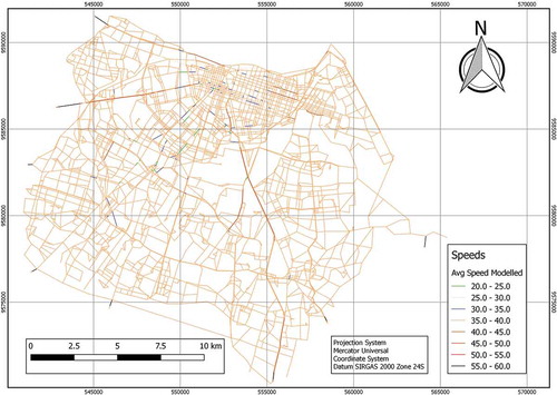
OSPM requires as inputs average traffic speeds in order to model air pollutants in street canyons (Kakosimos et al. 2010). TRANUS travel demand model was capable of estimate average travel speed in Fortaleza region and exported to shape-file, necessary as input to OSPM. In this regard, the road network with modeled average travel speeds of Fortaleza main streets is shown in Figure 4.

Figure 4. Road network with travel speeds (km/h) in all streets of the municipality of Fortaleza, CE

Calibration of average daily traffic flows has been carried out with the inductive loop-type sensor for traffic data collection using the SCOOT system. TRANUS was calibrated to estimate AADT for all streets in Fortaleza and several parameters can interfere in traffic estimations, such as activity system and land use (de la Barra 1982). Uncertainties in estimated AADT can be observed and influence air pollutant concentrations in street levels estimated by OSPM. The modeled traffic flow and observed traffic flow (used to calibrate travel demand model) of major streets inside and outside the case study area are shown in Table 3.

Table 3. Observed and modeled average daily traffic flows in major streets of Fortaleza

Street/Avenue	Modeled	Observed	Difference	Relative Error (%)
Washington Soares	52,625	50,239	2386	+5
Santos Dumont	44,671	42,607	2,064	+5
Antônio Sales	26,934	34,280	−7,346	−21
Presidente Castelo Branco	46,736	40,439	6,297	+16
Padre Antônio Tomás	39,909	38,745	1,164	+3.
Padre Valdevino	27,967	20,936	7,031	+34
Sen. Virgílio Távora	31,637	30,980	657	+2
Br. De Studart	25,292	31,501	−6,209	−20
Rui Barbosa	15,626	18,484	−2,858	−15
Ana Bilhar	22,828	23,006	−178	−1

The difference between modeled and measured traffic flows shows both under- and overestimations with modeled traffic flows within −21% to 34% of measured traffic flows due to uncertainties of AADT modeling in a city the size of Fortaleza.

Meteorological data and regional background concentrations

The characteristics of meteorological data in Fortaleza are shown in Table 4. The mean temperature (T) in 2017 was normal (mean ± SD: 28.3 ± 2.2°C), while the relative humidity (RH) was high (76.1 ± 12.8%). In addition, the precipitation intensity (PI) was normal for the city (0.2 ± 1.2 mm/h). The collected and calculated meteorological parameters were used in combination with regional background concentrations to estimate urban background concentrations using UBM.

Table 4. Characteristics of meteorological data collected and calculated hourly for year 2017. Temperature (T), Relative Humidity (RH), Precipitation Intensity (PI), Air Density (AD), Wind Speed (WS), and Global Radiation (GR) were field data collected by FUNCEME. Mixing Height (MH), Monin-Obhukov Length (M-OL), Convective Velocity (CV), and Friction Velocity (FV) were calculated using OML-Highway meteorological Pre Processor

Statistics	T (°C)	RH (%)	PI (mm/h)	AD (kg/m^3)	WS (m/s)	GR (W/m^2)	MH (m)	M-O L (m)	CV (m/s)	FV (m/s)
Mean	28.3	76.1	0.2	1.2	3.9	236.5	474.7	25.5	0.3	0.2
Standard Error	0.02	0.1	0.01	0	0.02	3.4	4.4	10.1	0.01	0
Kurtosis	−0.6	−0.5	328.4	−0.6	−0.8	−0.4	4.6	82.8	0.8	3.9
Skewness	0.3	−0.3	14.9	−0.1	0.04	1.0	1.9	1.9	1.4	1.7
Range	11.9	63.6	40.8	0.1	9.3	1,071.1	3,108	19,998	2.9	1.5
Minimum	22.4	36.7	0	1.1	0	0	150	−9,999	0	0.03
Maximum	34.3	100.3	40.8	1.2	9.3	1,071.1	3258	9,999	2.9	1.6
Count	8,760	8,760	8,760	8,760	8,760	8,760	8,760	8,760	8,760	8,760

Regional background air pollutant concentrations were available for the whole year of 2017; however, meteorological data for the air quality calculations for UBM and OSPM only consider the two measurement campaign periods (May, July, and November) for NO₂ and PM₁₀.

Gridded vehicle emissions for modeling urban background concentrations

Gridded vehicle emissions in tons/year are needed as input to UBM to be able to model urban background concentrations. NO_x and total PM₁₀ emissions (exhaust and non-exhaust) are required. A grid with grid cells of 1 km x 1 km was defined for the case study area using GIS to be able to model vehicle emissions. The emissions of each grid cell were calculated based on data on road length, traffic flow, travel speed, vehicle distribution and emission factors of different emission technology layers (Pre-EURO to EURO 5) and further depending on vehicle type and fuel type. In Figure 5, the percentage of vehicle emissions in Fortaleza is shown broken down by vehicle type and fuel type and emission technology layer.

Figure 5. NO_x (a) and PM₁₀ (b) emission contributions (%) for traffic conditions in the Fortaleza vehicle fleet. PM₁₀ contributions includes exhaust and non-exhaust particles of mobile emissions

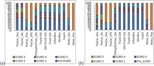
Variability in emission contributions for a given vehicle type are results of different reasons in this study: proportional fuel used (e.g., passenger cars using gasoline, ethanol, mixture of both, or LPG; motorcycles using gasoline or mixture of gasoline and ethanol); age of manufacturing (which also change fuel used); vehicle engine sizes (e.g., trucks and buses with three different sizes mentioned in Figure 5, in addition to age of manufacturing). Variations in emission contributions among emission standards for a given pollutant and vehicle type are results of fleet age of manufacturing (real data used).

Passenger cars have been disaggregated by fuel type: gasoline, alcohol, flex, and LPG. Pickups, SUVs, and vans use diesel. Trucks were sub-divided in less than 10 tons, between 10 and 15 tons, and plus 15 tons (all diesel). Buses are subdivided in urban buses, coaches, and mini buses (all diesel). Motorcycles were divided in gasoline and flex fueled. Brazilian emission standards (PROCONVE standards) have been converted to equivalent EURO standards (CONAMA, 2017; ICCT, 2016). It is important to note that Flex vehicles are the most numerous in the Fortaleza fleet; however, around 90% of them use gasoline due to economic reasons as gasoline is cheaper than ethanol (Fortaleza 2015).

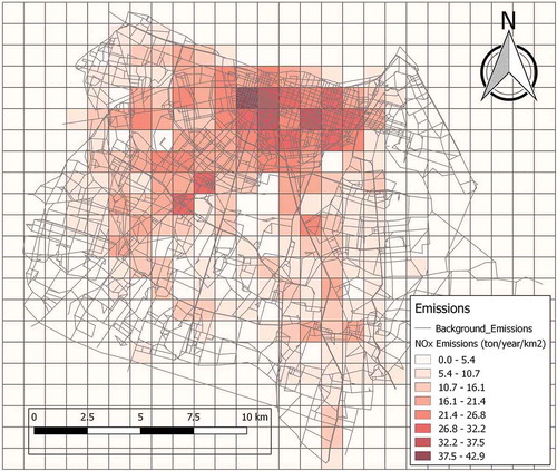
Spatial distribution of gridded vehicle emissions (1 x 1 km) for NO_x is shown in Figure 6. The highest emissions are in the north part of Fortaleza due to high density of roads and high traffic flows, as observed by Oliveira et al. (2019) with 13 Urban Recreation Areas (URAs) data collection points experiment.

Figure 6. NO_x emissions from traffic in Fortaleza in 2017 based on adjusted emission factors (ton/year/km²). The same spatial pattern is also observed for PM₁₀ emissions

Results

Modeling urban background concentrations

Urban background concentrations were modeled with UBM based on the gridded vehicle emissions, regional background concentrations and meteorological data for the whole year of 2017, and hence also for the two campaign periods. Urban background concentrations are used as input to model street concentrations with OSPM. In what follows, we show results based on adjusted emission factors.

Adjustments in UBM have been carried out similarly to research presented in Valencia et al. (2019), where emission inputs can be used to calibrate both NO_x and PM₁₀. Ideally, these factors must have the value of one; higher values increase the emissions and produce higher concentrations, and the opposite is valid. In this study, UBM adjustments considering OSPM default emission factors have been calculated with NO_x = 1.5 and PM₁₀ = 4.0. In the scenario with OSPM adjusted emission factors (Krecl et al. 2018), UBM factors were calculated with the value of one with satisfactory good results.

Results are illustrated with average over the campaign period and daily for urban background concentrations and compared to regional background data for the first campaign in Figure 7. Meteorological data shows that the first campaign is the rainy season in Fortaleza and the second campaign shows the dry season in the studied area; however, in order to illustrate underestimations in street pollution modeling during rainy days, the first campaign has been highlighted in data and figures.

Figure 7. Daily and average NO_x, NO₂, O₃, and PM₁₀ urban background concentrations in Fortaleza based on UBM (µg/m³), calculated with adjusted emission factors, presented in (a), (c), (e), and (g). Regional background concentrations presented to compare with urban background concentrations (b), (d), (f), and (h)

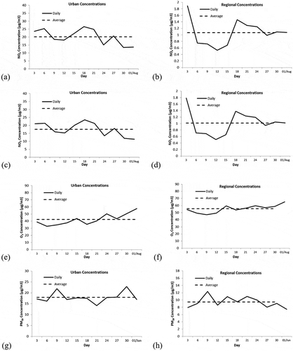
Temporal variation of background pollution concentrations is influenced by the meteorological parameters. Regional NO_x, NO₂, and O₃ concentrations showed variations probably due to wind direction changes and higher wind speeds in the month of July (reduction or increasing of source areas), and PM due to precipitation days during the month of May (PM washout) (Akyuz et al., 2009; Barmpadimos et al. 2011). Urban concentrations follow regional concentration patterns, with urban mobile sources increment.

As expected the urban background concentrations are much higher than the regional background concentrations for NO_x and NO₂ as traffic is a major source of NO_x emissions. It is also seen that regional background ozone concentrations are higher than urban background ozone concentrations as NOx emissions in the city deplete ozone. For PM₁₀ the regional background concentration is relatively high compared to the urban background concentration of PM₁₀, due to seasalt contributions in Fortaleza (the city is close to the sea). PM₁₀ regional background concentrations are proportionally much higher when compared to NO_x and NO₂ due to the same reasons previously mentioned.

Evaluation of modeled street concentrations with OSPM against air quality measurements

Street concentrations were modeled with OSPM for selected streets based on traffic data, street configuration data, modeled urban background concentrations, and meteorological data. Calculations were carried out with two sets of vehicle emission factors for OSPM. First, with default emission factors based on CETESB and with adjusted emissions for UBM (Scenario 3); secondly, with adjusted emission factors for OSPM and default emissions for UBM (Scenario 4).

Based on default vehicle emission factors for OSPM and adjusted emissions for UBM (Scenario 3)

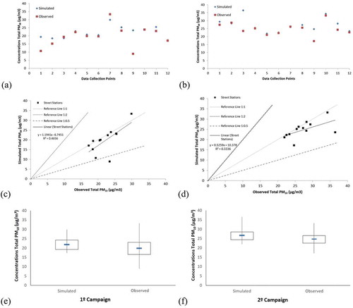
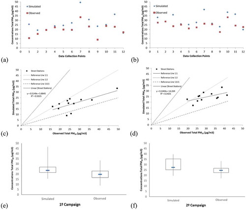
Figures 8 and Figures 9 show OSPM estimated concentrations of NO₂ and PM₁₀ compared to observed air quality data (24 hours) collected during the two campaigns (2017). Table 5 shows that mean simulated NO₂ concentration was higher in the first campaign in July (mean ± SD: 27.5 ± 6.2) compared to the second campaign in November (23.9 ± 6.5). Observed concentrations showed the same pattern in the first campaign (28.9 ± 17.8) compared to the second campaign (19.8 ± 9.9). In the case of PM₁₀, the mean simulated concentration was lower in the first campaign in May (22.2 ± 3.7) when compared to the second campaign in November (27.3 ± 4.4), and the same pattern was also seen for measured concentrations in first campaign (19.7 ± 6.5) compared to the second campaign (24.7 ± 4.1). Meteorological and traffic factors show large influence on measured and simulated results. Streets with high AADT and days with lower wind speeds show higher concentrations, and days with precipitation show lower concentrations, especially for PM₁₀. In the second campaign (November), there was almost no rain in Fortaleza and hence no washout of PM in the atmosphere. This may be the reason why PM₁₀ is better in agreement with the measurements in the second campaign compared to the first campaign as OSPM does not take into account PM washout. A good correlation existed between the mean of all observations and simulations, although the model overestimated for NO₂ in the second campaign. The good agreement between the mean of all observations and simulations is a result of the calibration of the emission factors for UBM to fit modeled street concentrations.

Table 5. Characteristics of simulated and observed concentrations during the two campaigns for NO₂ and PM₁₀. Simulated concentrations have been calculated using default emission factors from CETESB

	1º Campaign (NO2) (µg/m^3)		2º Campaign (NO2) (µg/m^3)		1º Campaign (PM10) (µg/m^3)		2º Campaign (PM10) (µg/m^3)
Statistics	Simulated	Observed	Simulated	Observed	Simulated	Observed	Simulated	Observed
Mean	27.5	28.9	23.9	19.8	22.2	19.7	27.3	24.7
Standard Error	1.5	4.2	1.5	2.2	1.1	1.9	1.3	1.8
Kurtosis	0.7	−0.5	−0.01	−0.3	0.1	1.0	0.4	1.2
Skewness	0.8	0.7	0.8	0.9	0.7	0.2	0.9	0.3
Range	23.6	59.8	23.3	34	12.7	24.4	14.5	16
Minimum	19.8	5.4	16	9.1	17.2	8.9	21.9	17.2
Maximum	42.8	65.2	39.3	43.1	29.9	33.3	36.5	33.2
Count	18	18	20	20	12	12	12	12
RMSE	15.2		9.0		5.2		4.5

Figure 8. Scenario 3. Simulated and observed NO₂ concentrations during two campaigns (July and November, 2017). (a) NO₂ in first campaign. (b) NO₂ in second campaign. (c) Scatter Plot of simulated and observed NO₂ data, 1º Campaign. (d) Scatter Plot of simulated and observed NO₂ data, 2º Campaign. (e) Boxplot of NO₂ concentrations in first campaign. (f) Boxplot of NO₂ concentrations in second campaign

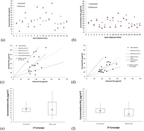
Figure 9. Scenario 3. Simulated and observed PM₁₀ concentrations during two campaigns (May and November, 2017). (a) PM₁₀ in first campaign. (b) PM₁₀ in second campaign. (c) Scatter Plot of simulated and observed PM₁₀ data, 1º Campaign. (d) Scatter Plot of simulated and observed PM₁₀ data, 2º Campaign. (e) Boxplot of PM₁₀ concentrations in first campaign. (f) Boxplot of PM₁₀ concentrations in second campaign

Based on adjusted vehicle emission factors for OSPM and default emissions for UBM (Scenario 4)

Figures 10 and Figures 11 and Table 6 show comparisons between simulated and observed street concentrations based on adjusted emission factors for OSPM and default emissions for UBM.

Table 6. Characteristics of simulated and observed concentrations calculated and collected in the two proposed campaigns, NO₂ and PM₁₀. Simulated concentrations have been calculated using adjusted emissions for OSPM and default emissions for UBM

	1º Campaign (NO2) (µg/m^3)		2º Campaign (NO2) (µg/m^3)		1º Campaign (PM10) (µg/m^3)		2º Campaign (PM10) (µg/m^3)
Statistics	Simulated	Observed	Simulated	Observed	Simulated	Observed	Simulated	Observed
Mean	29.8	28.9	26	19.8	25.5	19.7	29.4	24.7
Standard Error	2.7	4.2	2.7	2.2	2.4	1.9	1.9	1.2
Kurtosis	0.3	−0.5	−0.3	−0.3	3.3	1.0	−1.2	1.2
Skewness	0.7	0.7	0.7	0.9	1.6	0.2	0.2	0.3
Range	42.3	59.8	42	34.0	31.1	24.4	20.1	16.0
Minimum	14	5.4	11.1	9.1	15.6	8.9	19.6	17.2
Maximum	56.3	65.2	53.0	43.1	46.7	33.3	39.7	33.2
Count	18	18	20	20	12	12	12	12
RMSE	15.5		13.5		9.3		7.6

Figure 10. Scenario 4. Simulated and observed NO₂ street concentrations in two campaigns (July and November, 2017). Simulated data with adjusted emission factors for OSPM and default emissions for UBM. (a) NO₂ in first campaign. (b) NO₂ in second campaign. (c) Scatter Plot of simulated and observed NO₂ data, 1º Campaign. (d) Scatter Plot of simulated and observed NO₂ data, 2º Campaign. (e) Boxplot of NO₂ concentrations in first campaign. (f) Boxplot of NO₂ concentrations in second campaign

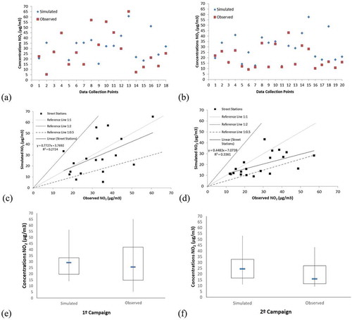
Figure 11. Scenario 4. Simulated and observed PM₁₀ street concentrationsin two campaigns (May and November, 2017). Simulated data with adjusted emission factors for OSPM and default emissions for UBM. (a) PM₁₀ in first campaign. (b) PM₁₀ in second campaign. (c) Scatter Plot of simulated and observed PM₁₀ data, 1º Campaign. (d) Scatter Plot of simulated and observed PM₁₀ data, 2º Campaign. (e) Boxplot of PM₁₀ concentrations in first campaign. (f) Boxplot of PM₁₀ concentrations in second campaign

Figures 10 and Figures 11 show similar correlations between observed and simulated concentrations as Figures 8 and Figures 9. However, the simulated street concentrations are higher in Scenario 4 compared to Scenario 3. The reason is that the street concentration is dominated by the street contribution (difference between street concentrations and background concentrations). In Scenario 4, we use adjusted emission factors for OSPM (default emissions for UBM) and hence the street contribution becomes much larger than in Scenario 3 (default emission for OSPM and adjusted for UBM).

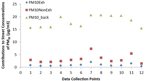
Figure 12 shows source apportionment of PM₁₀ street concentrations in selected streets based on OSPM with adjusted emission factors and UBM with default emissions. It is seen that the urban background concentrations are a major contributor to PM₁₀ street concentrations where about half originates from the regional background (Figure 7). Additionally, non-exhaust particles contribute much more than exhaust particles.

Figure 12. Source apportionment of PM₁₀ street concentrations. PM10_back is the urban background concentrations, PM10Exh is the exhaust part, and PM10NonExh the non-exhaust part calculated with OSPM

Discussion

It was possible to modify the emission module of OSPM to match all five vehicle types used in this study for Brazilian conditions. Air quality calculations were carried out with two sets of vehicle emission factors. First, with official Brazilian default emissions factors based on CETESB, and secondly, with adjusted higher emission factors based on calibration of emissions for UBM to fit the average measured street concentrations. The adjusted emission factors were close to adjusted emission factors proposed by Krecl et al. (2018). Non-exhaust PM₁₀ emissions are not included in the official Brazilian emission factors, and hence non-exhaust emission factors were taken from the European COPERT IV emission model (EEA, 2016).

On average, modeled street concentrations showed relatively good agreement with measurements when using the default vehicle emission factors for OSPM and adjusted emission for UBM (Scenario 3). This is also expected, as it is a result of the calibration of emissions for UBM to fit measured street concentrations. It is also expected that modeled street concentrations are overestimated in Scenario 4 with adjusted emissions for OSPM and default for UBM since the street contribution becomes overestimated. In Scenario 1 with default emissions for both UBM and OSPM, street concentrations were largely underestimated, and in Scenario 2 with adjusted emission for both UBM and OSPM, street concentrations were largely overestimated (data not shown). This indicates that the derived adjusted emission factors are too high although they are similar to those proposed by Krecl et al. (2018). However, based on the modeled street concentrations and observations in this study, it is not possible to firmly conclude which vehicle emissions represent real emissions due to lack of measurements for validation of the modeled urban background concentrations and modeled regional background concentrations. It could also be that the regional background concentrations used as input to UBM are too low or too high. Regional background concentrations showed high concentrations of ozone (O₃) and particles (Figure 6) due to transport of anthropogenic emissions (industrial and transportation) as well as seasalt, organic matter, and black carbon from the Fortaleza region (Flemming and Huijnen 2011). In addition, low regional concentrations of NO_x (NO + NO₂) have been observed. It has not been possible to validate the modeled regional background concentrations against measurements as no air quality monitor station exists that represents regional background concentrations to Fortaleza. Hence, it is not possible to assess if regional background concentrations are under- or overestimated. The same is the case for modeled urban background concentrations as no air quality monitor station exists to represent urban background. Contributions from industrial emissions were not analyzed. However, the contributions to Fortaleza from stationary sources are expected to be relatively low due to the location of the industrial sources outside the city and the dominant wind directions, reported by Silva et al. (2017).

Modeled contributions to PM₁₀ exhaust, PM₁₀ non-exhaust, and urban background concentrations of PM₁₀ are comparable to other related PM contribution studies (Wang et al. 2010; Harrison et al. 2012; Lutz 2013; Cyrys et al. 2014; Holman, Harrison, and Querol 2015). However, all in all, the default and also adjusted vehicle emissions are likely to remain uncertain. While non-exhaust emission have been relative constant over the last years, in contrary exhaust emission have been substantially reduced for example by the introduction of particle filters and improved engine technology. As a result, the relative contribution of non-exhaust emission compared to exhaust emissions has been increasing over time, and today non-exhaust emissions predominate over the exhaust kind.

With relative errors in traffic flows of −22% to +34% in comparison with observations, as also mentioned in another reported study (Sousa, 2016). Under- and overestimations in modeled traffic flows are due to uncertainties in measurements of traffic data collected by CTAFOR and simulations with the travel demand model. Vehicle distributions were based on traffic counts and travel speed on travel demand modeling. In summary, the uncertainties on traffic data are assessed to be modest compared to other elements in the model chain.

Meteorological parameters estimated by the IFS model were consistent with the official Fortaleza meteorological data collection (Funceme 2018). Parameters obtained, such as temperature, precipitation, wind speed, and wind direction have low uncertainties whereas calculated parameters, such as mixing height have higher uncertainty, although it was shown to directly correlate with NO₂ and PM₁₀ as mentioned in previous studies (Banerjee and Srivastava 2009; Seo et al. 2017; Zheng et al. 2015).

Observed NO₂ street concentrations showed higher values in the first campaign when compared to the second campaign and the same was seen in the simulated NO₂ concentrations (Figure 7 and Table 4). One of the potential reasons for higher NO₂ concentrations in July was the higher concentrations of ozone (O₃) leading to formation of NO₂ through reaction with NO during this period (Fowler et al. 1999, 1998). Lower mixing height was observed in the first campaign, which will slightly increase NO₂ concentrations, as mentioned in previous studies (Dieudonné et al. 2013).

Observed PM₁₀ concentrations showed higher values in the second campaign also reproduced in the simulated PM₁₀ concentrations (Figure 8 and Table 4). One of the potential reasons for this increase in concentrations could be the effect of temperatures on gas-to-particle conversion (Sheehan and Bowman 2001; Strader, Lurmann, and Pandis 1999). Furthermore, lower temperatures in the rainy season could be observed in the meteorological parameters leading to lower mixing heights (convective boundary layer depth), also confirmed in a previous study (Pal et al. 2012). Lower mixing heights will, other things equal, result in higher concentrations of atmospheric particles (Tiwari et al. 2014).

In addition, PM₁₀ measurements showed outlier concentrations at data collection points 1 and 9 (lower concentrations). These outliers could be observed due to strong rainfall during the data collection days in the rainy season in May. Many studies on precipitation washout of PM in the air are reported with comparison between particulate matter concentrations under conditions of precipitation and non-precipitation (Akyuz and Cabuk 2009; Barmpadimos et al. 2011). However, OSPM simulated concentrations overestimate PM₁₀ concentrations under such conditions as washout of PM is not modeled in OSPM. Outliers in simulations at data collection points 7 and 11 (higher concentrations) were seen due to low calculated mixing height during most of the simulated day, which can differ from the actual mixing height. However, in general, simulated PM₁₀ concentrations followed the variation in observed concentrations.

There are also limitations concerning measurements. First, the locations, number, and days of data collected were relatively low due to lack of budget and free public data. Second, the measurements of NO₂ may be uncertain as they was based on passive sampler methodology. Third, the absence of air quality monitoring data for regional and urban background concentrations made it impossible to validate modeled regional background concentrations and modeled urban background concentrations.

Conclusion

This study presents the comparison between modeled street concentrations and measurements of NO₂ and PM₁₀ at selected streets in Fortaleza. The wider aim is to develop a model system for decision-support estimating the effects of potential traffic-related measures such as the introduction of Low Emission Zones.

In one of the tested model set-up scenarios, Scenario 3 with adjusted emissions for UBM based on calibration and default emissions for OSPM, the system agreed well with observations on average. In Scenario 4 with default emissions for UBM and adjusted emissions for OSPM, the model overestimated observations as expected. However, based on the modeled street concentrations and observations it is not possible to conclude which vehicle emissions represent the most realistic emissions due to a lack of measurements at urban background and regional background levels. Hence, it is not possible to assess whether or not regional and urban background concentrations are under- or overestimated. This illustrates the difficulties to disentangle the uncertainties on the different contributions (regional, urban background, and street) when observations are only available for street concentrations. In future research, concentration data should be collected simultaneously at kerbside, urban background, and regional background location. Such data could help to further estimate the contributions of vehicle emissions on many roads with different traffic volumes and vehicle type composition in street concentrations.

However, given the scenario calculations in relation to observations, there are indications that official Brazilian default emissions are too low but also that the adjusted emissions derived in this project are too high. The findings in this research could contribute to strengthening the management of traffic-related air pollution in Fortaleza. Furthermore, based on the findings of this study, the local governments of other developed cities in Brazil, such as São Paulo, Rio de Janeiro, and Curitiba, could take advantage of the developed methodology to evaluate the effect of potential measures to reduce air pollution.

Acknowledgment

The authors thank the Coordenação de Aperfeiçoamento de Pessoal de Nível Superior--Brasil (CAPES), for its financial support to this PhD project. The authors are also grateful to Fundação Cearense de Meteorologia e Recursos Hídricos (FUNCEME) for provided data. The first author also thanks the Department of Environmental Science at Aarhus University in Denmark for hosting an 8-month research stay at the department as part of his Ph.D. study.

Disclosure statement

No potential conflict of interest was reported by the authors.

Additional information

Notes on contributors

Helry L.F. Dias

Helry L.F. Dias is Ph.D. in Transportation Engineering, Adjunct Professor of Transportation and Logistics Engineering at Federal University of Santa Catarina.

Bruno V. Bertoncini

Bruno V. Bertoncini is Ph.D. in Transportation Engineering, Adjunct Professor in Transportation Engineering at Federal University of Ceará.

Rivelino M. Cavalcante

Rivelino M. Cavalcante is Ph.D. in Organic Chemistry, Associate Professor at Federal University of Ceará.

Steen Solvang Jensen

Steen Solvang Jensen is Ph.D. from the Institute of Environment, Technology and Social Studies, University of Roskilde, Denmark, Head of Section, Section of Atmospheric Environment, Department of Environmental Science and Senior Scientist, Department of Environmental Science, Aarhus University, Denmark.

Kaj M. Hansen

Kaj M. Hansen is Ph.D. in Geophysics, degree from the Niels Bohr Institute for Astronomi, physics and geophysics and the COGCI PhD-school, Faculty of Science, University of Copenhagen, Scientist, Department of Atmospheric Environment, National Environmental Research Institute.

Matthias Ketzel

Matthias Ketzel is Ph.D. in Physics, Lund University, Sweden, Senior Scientist at Aarhus University and Visiting Professor at Global Centre for Clean Air Research (GCARE), University of Surrey.

References

- Akyuz, M., and H. Cabuk. 2009. Meteorological variations of PM2.5/PM10 concentrations and particle-associated polycyclic aromatic hydrocarbons in the atmospheric environment of Zonguldak, Turkey. J. Hazard. Mater. 170(1), 13–21. doi: 10.1016/j.jhazmat.2009.05.029
- Alam, M. D. S., B. Hyde, P. Duffy, and A. McNabola. 2017. An assessment of Pm 2.5 reductions as a result of transport fleet and fuel policies addressing CO2 emissions and climate change. Air Pollution XXV. WIT Transactions on Ecology and The Environment, 211, WIT Press. www.witpress.com, 1746-448X (on-line)
- Alcântara, A. P. M. P., J. P. Ribeiro, L. M. Barbosa, V. T. F. Castelo Branco, B. V. Bertoncini, and R. M. Cavalcante. 2019. Avaliação da emissão de material particulado e dióxido de nitrogênio na usinagem de misturas asfálticas. 33º Congresso de Ensino e Pesquisa em Transporte da ANPET. Balneário Camboriú-SC.
- Alves, A. S. 2014. Avaliação da operação do sistema de detecção veicular por vídeo e por indução aplicados ao sistema SCOOT. Monografia (Especialização em Gestão de Trânsito e Transportes Urbanos) - Departamento de Engenharia de Transportes, Universidade Federal do Ceará, Fortaleza.
- Andrade, M. F., R. Y. Ynoue, E. D. Freitas, E. Todesco, A. Vara-Vela, S. Ibarra, L. D. Martins, J. A. Martins, and V. S. B. Carvalho. 2015. Air quality forecasting system for Southeastern Brazil. Front. Environ. Sci. 3, 1.
- Banerjee, T., and R. K. Srivastava, Evaluation of ambient air quality at IIE Pantnagar and its surroundings through combined air quality index. International Symposium on Environmental Pollution, Ecology and Human Health, Tirupati, India (2009).
- Barmpadimos, I., C. Hueglin, J. Keller, S. Henne, and A. S. H. Prevot. 2011. Influence of meteorology on PM10 trends and variability in Switzerland from 1991 to 2008. Atmos. Chem. Phys. 11, 1813–35.
- Berkowicz, B., M. Ketzel, S. S. Jensen, M. Hvidberg, and O. Raaschou-Nielsen. 2008. Evaluation and application of OSPM for traffic pollution assessment for large number of street locations. Environ. Model. Softw. 23 296–303.
- Berkowicz, R. 2000a. OSPM – A parameterised street pollution model. Environ. Monit. Assess. 65 (1/2), 323–31.
- Berkowicz, R. 2000b. A simple model for urban background pollution. Environ. Monit. Assess., 65, 1–2, 259–67. doi: 10.1023/A:1006466025186.
- Berkowicz, R., H. Olesen, and S. S. Jensen. 2003. User’s guide to WinOSPM: Operational street pollution model. NERI Technical Report. National Environmental Research Institute, Roskilde, Denmark.
- Berkowicz, R., O. Hertel, S. E. Larsen, N. N. Sørensen, and M. Nielsen. 1997. Modeling traffic pollution in streets. NERI Report. National Environmental Research Institute, Roskilde, Denmark.
- Brandt, J., J. H. Christensen, L. M. Frohn, and R. Berkowicz. 2003. Air pollution forecasting from regional to urban street scale – Implementation and validation for two cities in Denmark. Physi. Chem. Earth 28, 335–44.
- Brito, J., S. Carbone, D. A. M. Santos, P. Dominutti, N. O. Alves, L. V. Rizzo, and P. Artaxo. 2018. Disentangling vehicular emission impact on urban air pollution using ethanol as a tracer. Sci. Rep, 8. doi: 10.1038/s41598-018-29138-7.
- Coelho., P. I. S. 2006. A Importância da Localização Aeroportuária na Qualidade do Ar - O Caso da Expansão do Aeroporto Santos Dumont na Cidade do Rio de Janeiro. 2006. Dissertação (Mestrado em Ciências em Engenharia de Transportes) - Programa de Pós-Graduação de Engenharia, Universidade Federal do Rio de Janeiro, Rio de Janeiro.
- Companhia Ambiental do Estado De São Paulo (CETESB). 2017a. Emissões veiculares no estado de São Paulo - 2016. Série Relatórios CETESB. São Paulo, Brasil.
- Conselho Nacional do Meio Ambiente (CONAMA). 2017. Limites máximos de emissão. Programa de Controle da Poluição do Ar por Veículos Automotores - PRONCOVE P8. Accessed 02 Aug 2018. <http://www.ibama.gov.br/phocadownload/proconve-promot/2017/consulta-publica/2017-10-proposta-conama-P8-%20final-mbv-v3.pdf>
- Controle de Tráfego em Área Urbana de Fortaleza (CTAFOR). 2015. Base de dados do ASTRID. Automatic SCOOT Traffic Information Database.
- Cristensen, J. H. 1997. The Danish eulerian hemispheric model — A three-dimensional air pollution model used for the arctic. Atmos. Environ. 31, 24, 4169–91. doi: 10.1016/S1352-2310(97)00264-1
- Cyrys, J., A. Peters, J. Soentgen, and H. E. Wichmann. 2014. Low emission zones reduce PM10 mass concentrations and diesel soot in German cities. JAWMA 64, 4, 481–87.
- Danish Center for Environment and Energy. 2014. Manual for thor-airpas- air pollution assessment system. Technical Report from DCE Nº 46. Roskilde, Denmark.
- Darcin, M. 2014. Association between air quality and quality of life. Environ. Sci. Pollut. Res. 21(3): 1954–59. doi: 10.1007/s11356-013-2101-3
- de la Barra, T. 1982. Modelling regional energy use: A land use, transport and energy evaluation model environment and planning B: Plann. Des., 9, 429–43
- de la Barra, T. 1989. Integrated land use and transport modelling Cambridge University Press, Cambridge
- de la Barra, T. 1998. Improved logit formulations for integrated land use, transport and environmental models. In Network infrastructure and the urban environment: recent advances in land-use/ transportation modelling (L. Lundqvist, L.-G. Mattsson, and T. J. Ki, eds.), 288–307 Springer, Berlin/Heidelberg/New York
- de la Barra, T., B. Pérez, and N. Vera. 1984. TRANUS-J: putting large models into small computers environment and planning b: planning and design, 11, 87–101
- Dieudonné, E., F. Ravetta, J. Pelon, F. Goutail, and J. P. Pommereau. 2013. Linking NO2 surface concentration and integrated content in the urban developed atmospheric boundary layer. Geophys. Res. Lett., 40, 1247–51, doi: 10.1002/grl.50242.
- European Environment Agency (EEA). 2016. Air quality in Europe — 2016 report. EEA Report Nº 28/2016. Copenhagen, Denmark.
- Flemming, J., and V. Huijnen. 2011. IFS tracer transport study, MACC deliverable G‐RG 4.2. Technical Report ECMWF. Monitoring Atmospheric Composition and Climate, MACC Project.
- Flemming, J., V. Huijnen, J. Arteta, P. Bechtold, A. Beljaars, A. M. Blechschmidt, M. Diamantakis, R. J. Engelen, A. Gaudel, A. Inness, et al. 2015. Tropospheric chemistry in the integrated forecasting system of ECMWF. Geosci. Model Dev., 8, 975–1003. doi: 10.5194/gmd-8-975-2015.
- Fortaleza. 2015. Base de Dados de Uso do Solo de Fortaleza. Fortaleza, Brazil.
- Fortaleza. 2018. Base de Dados de Uso do Solo de Fortaleza. Brazil: Fortaleza. https://www.fortaleza.ce.gov.br/a-cidade
- Fowler, D., C. Flechard, U. Skiba, M. Coyle, and J. N. Cape. 1998. The atmospheric budget of oxidized nitrogen and its role in ozone formation and deposition. New Phytol., 139, 11–23.
- Fowler, D., J. N. Cape, M. Coyle, R. I. Smith, A. G. Hjellbrekke, D. Simpson, R. G. Derwent, and C. E. Jonhson. 1999. Modelling photochemical oxidant formation, transport, deposition and exposure of terrestrial ecosystems. Environ. Pollut., 100, 43–55.
- Funceme. 2018. Monitoramento de dados meteorológicos do Estado do Ceará. Fortaleza, Brazil. accessed January 30, 2020. http://www.funceme.br/index.php/instituicao/monitoramento>
- Harrison, R. M., A. M. Jones, J. Gietl, J. Yin, and D. C. Green. 2012. Estimation of the contributions of brake dust, tire wear, and resuspension to nonexhaust traffic particles derived from atmospheric measurements. Environ. Sci. Technol. 46, 6523–29.
- Holman, C., R. M. Harrison, and X. Querol, 2015. Review of the efficacy of low emission zones to improve urban air quality in European cities. Atmos. Environ., 111, 161–69. doi: 10.1016/j.atmosenv.2015.04.009.
- Instituto Brasileiro de Geografia e Estatística (IBGE), Fortaleza. 2018. Panorama populacional de Fortaleza. acessed January 31, 2020. https://cidades.ibge.gov.br/brasil/ce/fortaleza/panorama
- International Council of Clean Transportation (ICCT). 2019. New concession bidding process could help soot-free and zero-emission buses in Campinas.
- International Council on Clean Transportation (ICCT). 2016. Deficiências no programa PROCONVE p-7 brasileiro e o caso para normas p-8. ICCT Análise de Políticas.
- Jensen, S. S., M. Ketzel, J. Brandt, M. Plejdrup, O. K. Nielsen, M. Winther, O. Evdokimova, and A. Gross. 2014. Manual for THOR-AirPAS - air pollution assessment system. Technical project Report for AirQGov Regional Pilot Project 3 (AirQGov:RPP3). Aarhus University, DCE – Danish Centre for Environment and Energy, 51 pp. Technical Report from DCE – Danish Centre for Environment and Energy No. 46. http://dce2.au.dk/pub/TR46.pdf
- Jensen, S. S., M. Ketzel, T. Becker, J. Christensen, J. Brandt, M. S. Plejdrup, M. Winther, O. K. Nielsen, O. Hertel, and T. Ellermann. 2017. High resolution multi-scale air quality modelling for all streets in denmark. Transp. Res. Part D Transp. Environ. 322–39. doi: 10.1016/j.trd.2017.02.019.
- Jensen, S. S., R. Berkowicz, H. S. Hansen, and O. Hertel. 2001. A Danish decision-support GIS tool for management of urban air quality and human exposures. Transp. Res. Part D Transp. Environ. 6, 229–41.
- Kakosimos, K. E., O. Hertel, M. Ketzel, and R. Berkowicz. 2010. Operational street pollution model (OSPM) - a review of performed validation studies, and future prospects. Environ. Chem., 7, 485–503. doi: 10.1071/EN10070.
- Ketzel, M., R. Berkowicz, H. Hvidberg, S. S. Jensen, and O. Raaschou-Nielsen. 2011. Evaluation of AirGIS - A GIS-based air pollution and human exposure modelling system. Int. J. Environ. Pollut. 47, 1/2/3/4, 2011. doi: 10.1504/IJEP.2011.047337.
- Ketzel, M., S. S. Jensen, J. Brandt, T. Ellermann, H. R. Olesen, R. Berkowicz, and O. Hertel. 2012. Evaluation of the street pollution model OSPM for measurements at 12 streets stations using a newly developed and freely available evaluation tool. J. Civ. Environ. Eng S 1:004.
- Krecl, P., A. Targino, C. Johansson, and J. Ström. 2015. Characterisation and source apportionment of submicron particle number size distributions in a busy street canyon. Aerosol Air Qual. Res., 15, 220–33. doi: 10.4209/aaqr.2014.06.0108
- Krecl, P., A. Targino, L. Wiese, M. Ketzel, and M. P. Corrêa. 2016. Screening of short-lived climate pollutants in a street canyon in a mid-sized city in Brazil. Atmos Pollut Res, 7, 6, 1022–36. doi: 10.1016/j.apr.2016.06.004
- Krecl, P., A. C. Targino, M. Ketzel, Y. A. Cipoli, and I. Charres. 2019. Potential to reduce the concentrations of short-lived climate pollutants in traffic environments: A case study in a medium-sized city in Brazil. Transp. Res. Part D. doi: 10.1016/j.trd.2019.01.032
- Krecl, P., A. C. Targino, T. P. Landi, and M. Ketzel. 2018. Determination of black carbon, PM2.5, particle number and NOx emission factors from roadside measurements and their implications for emission inventory development. Atmos. Environ. 186, 229–40. doi: 10.1016/j.atmosenv.2018.05.042.
- Li, M., and L. Mallat, 2018.SCOR Global Life, The Art & Science of Risk. Health Impacts of Air Pollution.
- Lopes, T. F. A., N. A. Policarpo, V. M. R. Vasconcelos, and M. L. M. Oliveira. 2018. Estimativa das emissões veiculares na região metropolitana de Fortaleza, CE, ano-base 2010. Engenharia Sanitária E Ambiental. 23 5. 1013–25. doi: 10.1590/S1413-41522018173312
- Loureiro, C. F. G., C. H. P. Leandro, and M. V. T. Oliveira. 2002. Sistema Centralizado de Controle do tráfego de Fortaleza: ITS Aplicado à Gestão Dinâmica do Trânsito Urbano. Anais do XVI ANPET - Congresso de Pesquisa e Ensino em Transportes, p. 19–26. Natal, RN.
- Lutz, M. 2013. Low emission zones & air quality in German cities, Clean Air Workshop, Berlin, September.
- Martins, E. M., J. D. N. Fortes, and R. A. Lessa. 2015. Modelagem de dispersão de poluentes atmosféricos: avaliação de modelos de dispersão de poluentes emitidos por veículos. Revista Internacional de Ciências, 5 (1):2–18. doi:10.12957/ric.2015.14498.
- Oliveira, M. G. 1997. Produção e Análise de Planos Semafóricos de Tempo Fixo usando Sistemas de Informações Geográficas. Dissertação de Mestrado, Universidade Federal do Rio de Janeiro, Rio de Janeiro.
- Oliveira, M. L. M., M. H. P. S. Lopes, N. A. Policarpo, C. M. A. C. Alves, R. S. Araújo, and F. S. A. Cavalcante. 2019. Avaliação de poluentes do ar em áreas de recreação urbana da cidade de Fortaleza. urbe. Revista Brasileira De Gestão Urbana, 11, e20180187. doi: 10.1590/2175-3369.011.e20180187
- Pal, S., I. Xueref-Remy, L. Ammoura, P. Chazette, F. Gibert, P. Royer, E. Dieudonné, J. C. Dupont, M. Haeffelin, C. Lac, et al. 2012. Spatio-temporal variability of the atmospheric boundary layer depth over the Paris agglomeration: An assessment of the impact of the urban heat island intensity. Atmos. Environ., 63, 261–75, doi: 10.1016/j.atmosenv.2012.09.046.
- Palmes, E. D., and R. H. Lindenboom. 1979. Ohm’s law, fickes law, and diffusion samplers for gases. Anal. Chem., 51 (14): 2400–01. doi: 10.1021/ac50050a026.
- Ribeiro, J. P., L. M. Barbosa, V. T. F. Castelo Branco, and R. M. Cavalcante. 2018. Avaliação da emissão de poluentes atmosféricos durante os processos de usinagem, transporte e aplicação de misturas asfálticas em ambiente urbano. 32º Congresso de Ensino e Pesquisa em Transporte da ANPET. Gramado-RS.
- Seo, J., J. Y. Kim, D. Youn, J. Y. Lee, H. Kim, Y. B. Lim, Y. Kim, and H. C. Jin. 2017. On the multiday haze in the Asian continental outflow: The important role of synoptic conditions combined with regional and local sources. Atmos. Chem. Phys., 17, 9311–32, doi: 10.5194/acp-17-9311-2017.
- Sheehan, P. E., and F. M. Bowman. 2001. Estimated effects of temperature on secondary organic aerosol concentrations. Environ. Sci. Technol., 35, 2129–35.
- Silva, G. K., A. C. S. Dos Santos, M. V. M. da Silva, J. M. B. Alves, A. C. B. Barbosa, C. L. Freire, C. R. Alcântara, and S. S. Sombra. 2017. Estudo dos Padrões de Ventos Offshore no Litoral do Ceará Utilizando Dados Estimados pelo Produto de Satélites BSW. Revista Brasileira De Meteorologia, 32 4, 579–690. doi: 10.1590/0102-7786324015
- Strader, R., F. Lurmann, and S. N. Pandis. 1999. Evaluation of secondary organic aerosol formation in winter, Atmos. Environ., 33, 4849–63.
- Superintendência Estadual do Meio Ambiente (SEMACE). 2016. Ceará opera com nova estação de monitoramento da qualidade do ar no CIPP. acessed January 31, 2020. https://www.semace.ce.gov.br/2016/12/14/ceara-opera-com-nova-estacao-de-monitoramento-da-qualidade-do-ar-no-cipp/
- Tiwari, S., D. S. Bisht, A. K. Srivastava, A. S. Pipal, A. Taneja, M. K. Srivastava, and S. D. Attri. 2014. Variability in atmospheric particulates and meteorological effects on their mass concentrations over Delhi, India, Atmos. Res., 145–146, 45–56, doi: 10.1016/j.atmosres.2014.03.027.
- United States Environmental Protection Agency (EPA). 2013. Integrated science assessment for oxides of nitrogen – health criteria (first external review draft) United States Environmental Protection Agency.http://cfpub.epa.gov/ncea/isa/recordisplay.cfm?deid=259167
- Valencia, H. V., O. Hertel, M. Ketzel, and G. Levin. 2020. Modeling urban background air pollution in Quito, Ecuador. Atmos Pollut Res, doi: 10.1016/j.apr.2019.12.014
- Vienneau, D., L. Perez, C. Schindler, C. Lieb, H. Sommer, N. Probst-Hensch, N. Kunzli, and M. Roosli. 2015. Years of life lost and morbidity cases attributable to transportation noise and air pollution: A comparative health risk assessment for Switzerland in 2010. Int. J. Hyg. Environ. Health 218(6): 514–21. doi: 10.1016/j.ijheh.2015.05.003
- Wang, F., M. Ketzel, T. Ellermann, P. Wåhlin, S. S. Jensen, D. Fang, and A. Massling. 2010. Particle number, particle mass and NO2 emission factors at a highway and an urban street in Copenhagen. Atmos. Chem. Phys. 10, 2745–64.
- Wegener, M., F. Gnad, and M. Vannahme. 1986. The time scale of urban change. In Advances in urban systems modelling (B. Hutchinson and M. Batty, eds.), 145–97. North Holland, Amsterdam
- World Health Organization (WHO). 2013. Review of evidence on health aspects of air pollution-REVIHAAP project: Final technical report. World Health Organziation Regional Office for Europe.
- World Health Organization (WHO). 2018. WHO global ambient air quality database, Accessed 27 Jan. 2020. https://www.who.int/airpollution/data/cities/en/
- Zheng, G. J., F. K. Duan, H. Su, Y. L. Ma, Y. Cheng, B. Zheng, Q. Zhang, T. Huang, T. Kimoto, D. Chang, et al. Exploring the severe winter haze in Beijing: The impact of synoptic weather, regional transport and heterogeneous reactions, Atmos. Chem. Phys., 15, 2969–83, doi: 10.5194/acp-15-2969-2015 2015