Long-term baseline ozone changes in the Western US: A synthesis of analyses

ABSTRACT

Quantification of the magnitude and long-term changes in ozone concentrations transported into the U.S. is important for effective air quality policy development. We synthesize multiple published trend analyses of western U.S. baseline ozone, and show that all results are consistent with an overall, non-linear change – a rapid increase (~5 ppb/decade) during the 1980s that slowed in the 1990s, maximized in the mid-2000s, and was followed by a slow decrease (~1 ppb/decade) thereafter. This non-linear change accounts for ~2/3 of the variance in 28 published linear trend analyses; we attribute the other 1/3 of the variance to unquantified autocorrelation in the analyzed data sets that result primarily from meteorologically driven interannual ozone variability. Recent systematic changes in baseline ozone on the U.S. West Coast have been relatively small – the standard deviation of the 2-year means over the 1990–2017 period is 1.5 ppb. International efforts to reduce anthropogenic precursor emissions from all northern mid-latitude sources could possibly reduce baseline ozone concentrations, thereby improving U.S. ozone air quality.

Implications: Ozone is an air pollutant with significant human and ecological health impacts. Air masses transported into the western U.S. from over the Pacific Ocean carry ozone concentrations that are, on average, a large fraction of the U.S. health standard. The US EPA policy assessment conducted for the recent review of the ozone National Ambient Air Quality Standard (NAAQS) found that 2016 regional average MDA8 ozone concentrations in the western US maximized in summer at ~52 ppb and that ~40 ppb of that maximum was contributed by ozone of natural and transported anthropogenic contributions. Thus, quantifying these trans-boundary background ozone concentrations has been identified as an important issue for a complete understanding of US air quality. Published analyses of temporal trends of these transported ozone concentrations vary widely, from early reports of increases to more recent reports of decreases. We show that the long-term ozone changes are nonlinear, with substantial concentration increases (as large as ~5 ppb/decade) before the mid-2000s when a maximum is reached, followed by a small decrease of ~1 ppb/decade thereafter. Superimposed on the overall changes is significant interannual variability that makes accurate determination of systematic trends over decade-scale time periods uncertain. The end of the previously increasing trends, and the recent decrease in transported ozone concentrations, is a good news for U.S. air quality, as it eases the difficulty of achieving the ozone air quality standard.

Introduction

Air masses from the Pacific marine environment enter the continental atmosphere over the western U.S. carrying ozone concentrations determined by natural and anthropogenic sources and sinks in the upwind regions. These transported ozone concentrations are large enough to significantly impact air quality in urban and rural U.S. locations; fully understanding this impact requires characterization of the temporal and spatial distribution of those ozone concentrations. The policy assessment (US EPA, 2020) conducted for the recent review of the ozone National Ambient Air Quality Standard (NAAQS) reviewed the current state of knowledge of this background ozone, and the November 2020 issue of EM (The Magazine for Environmental Managers published by A&WMA) was devoted to articles exploring the strengths and limitations of tools that can quantify background ozone. Over the past two decades, a number of observational-based studies have quantified the changes in average surface ozone concentrations at specific western U.S. locations thought to represent the background ozone in transported marine air; Table 1 lists 28 of these quantifications. Reported average trends over different time periods vary widely, from relatively large increases to smaller magnitude decreases. Our goal in this study is to synthesize these disparate results and to develop a consistent picture of the overall, decadal-scale temporal change in the transported ozone concentrations over the past 3 to 4 decades at the U.S. west coast.

Table 1. Slopes derived from published trend analyses (with 95% confidence limits) compared with slopes calculated from the quadratic fit to the northern mid-latitude analysis over the same time periods. Studies included report results based on mean or median annual or springtime seasonal data

Location	b (slope) (ppb decade^−1)	slope from quadratic fit (ppb decade^−1)	Years of data	Reference
Mid-troposphere	1.3 ± 0.9	0.1 ± 1.1	1994–2016	Gaudel et al. (2020)
Lower troposphere	−0.2 ± 0.9	0.1 ± 1.1	1994–2016	“
Centennial, Wyoming	−0.6 ± 0.9	0.8 ± 0.9	1989–2017	Cooper et al. (2020)
Great Basin NP	0.5 ± 0.9	0.1 ± 1.1	1993–2017	“
Gothic, Colorado	−1.0 ± 0.6	0.8 ± 0.9	1989–2017	“
Grand Canyon NP	−0.3 ± 0.7	0.8 ± 0.9	1989–2017	“
Centennial, Wyoming	−1.5 ± 1.2	−0.3 ± 1.2	1995–2017	“
Great Basin NP	0.2 ± 1.0	−0.3 ± 1.2	1995–2017	“
Gothic, Colorado	−1.9 ± 0.8	−0.3 ± 1.2	1995–2017	“
Grand Canyon NP	−1.5 ± 0.8	−0.3 ± 1.2	1995–2017	“
Centennial, Wyoming	−2.6 ± 1.8	−1.2 ± 1.4	2000–2017	“
Great Basin NP	−0.5 ± 1.4	−1.2 ± 1.4	2000–2017	“
Gothic, Colorado	−2.8 ± 1.1	−1.2 ± 1.4	2000–2017	“
Grand Canyon NP	−2.6 ± 1.1	−1.2 ± 1.4	2000–2017	“
Great Basin NP ^1	2.9 ± 2.3	0.4 ± 1.0	1994–2014	Lin et al. (2017)
Yellowstone NP ^1	2.1 ± 1.9	1.8 ± 0.7	1988–2012	“
Pinedale Wyoming ^1	0.9 ± 1.8	1.5 ± 0.7	1990–2012	“
Mesa Verde NP ^1	3.0 ± 1.8	0.8 ± 0.9	1994–2012	“
Mid-troposphere ^2	3.1 ± 2.1	0.2 ± 1.0	1995–2014	Lin et al. (2015)
Mid-troposphere ^2	4.2 ± 1.7	2.2 ± 0.6	1984–2014	“
Pacific MBL	2.7 ± 0.8	2.2 ± 0.6	1988–2010	Cooper et al. (2014)
Lassen Volcanic NP	2.7 ± 1.3	2.2 ± 0.6	1988–2010	“
Mid-troposphere ^2	4.1 ± 2.7	0.8 ± 0.9	1995–2011	Cooper et al. (2012)
Mid-troposphere ^2	5.2 ± 2.0	2.7 ± 0.6	1984–2011	“
Mid-troposphere ^2	6.3 ± 3.4	1.3 ± 0.8	1995–2008	Cooper et al. (2010)
Mid-troposphere ^2	7.0 ± 2.2	3.3 ± 0.6	1984–2008	“
Pacific MBL	3.4 ± 0.9	2.9 ± 0.5	1987–2007	Parrish, Millet, and Goldstein (2009)
Lassen Volcanic NP ^3	5.5 ± 2.7	3.6 ± 0.6	1988–2002	Jaffe et al. (2003)

¹Lin et al. (2017) results are taken from their Figure 13 for stations west of the Front Range of the Rocky Mountains.

²Results given for 50^th percentiles of the springtime seasonal data sets.

³Jaffe et al. (2003) results are 4 season average from full seasonal data sets in their Table 2.

Table 2. Parameter values (with 95% confidence limits) derived from quadratic fits for northern mid-latitudes and for two data sets collected in the western US (Parrish et al. 2020). Intercept and slope are given for the year 2000

Location	a (intercept)^1 (ppb)	b (slope) (ppb/decade)	c (curvature) (ppb/decade^2)	yearmax	Years of data
Northern mid-latitudes	–	2.0 ± 0.6	−1.8 ± 0.6	2005.7 ± 2.5	1978–2017
Lassen Volcanic NP	41.0 ± 0.7	2.6 ± 0.7	−2.4 ± 0.8	2005.4 ± 2.2	1987–2017
Pacific MBL	32.9 ± 1.1	1.4 ± 1.0	−2.5 ± 1.1	2002.8 ± 2.2	1987–2017
derived from trends	–	3.4 ± 0.9	−2.9 ± 0.8	2005.8 ± 2.2	1984–2017

¹A value for a is not returned for the fit to the normalized monthly means and the linear fit to the published trends.

A conceptual picture provides a useful framework for understanding the temporal variation of ozone at northern mid-latitudes. Prevailing westerly winds dominate atmospheric transport in this zonal band. On average, a circulating current of air repeatedly passes over all continents and oceans. The circum-global transport time is about 25–30 days, as indicated by a simple tracer experiment of a surface release using a global Lagrangian chemistry-transport model (STOCHEM-CRI; Derwent et al. 2018) driven by 1998 meteorological fields from the UK Meteorological Office Unified Model archive (Collins et al. 1997). The average lifetime of ozone in the free troposphere at these latitudes is longer than this transport time. The STOCHEM-CRI model finds that the northern mid-latitude ozone lifetime is about 50–60 days, when only loss processes are considered Figure 1b. However, in situ ozone production from photochemical oxidation of precursor compounds proceeds simultaneously with the photochemical and dry deposition loss processes and ozone is nearly in balance, so the mean net lifetime of ozone in an isolated air parcel at northern mid-latitudes is several months or longer. Meridional eddy fluxes of ozone can lead to perturbations of local concentrations, but on average the meridional gradients of ozone are small between 30 N and 60 N (e.g., Figure 2 of Crutzen, Lawrence, and Pöschl 1999), as are the mean meridional winds (e.g., Figure 7.17 of Peixoto and Oort 1992); thus, meridional advection does not, on average, significantly affect the mid-latitude budget of tropospheric ozone (see Supporting Information Section S1 for greater detail).

Figure 1. Long-term changes in baseline ozone at northern mid-latitudes. (a) Normalized, deseasonalized monthly mean data (gray points) from eight baseline data sets collected at the surface and in the free troposphere in western North America and western Europe. The symbols with error bars are 2-year means with standard deviations of the gray points, the black solid curve is a quadratic polynomial fit to the gray points. The colored curves are quadratic fits from analyses of two western US data sets (.Parrish et al. 2020). (b) Quadratic fit and 2-year means from (a) compared to line segments representing the annotated trend determinations from western US data sets covering varying time periods and included in Table 1

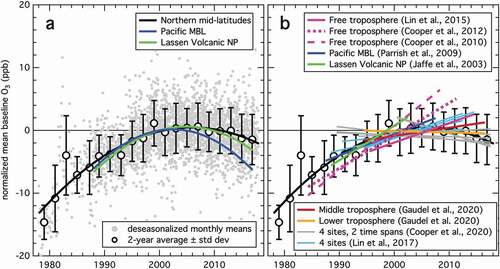
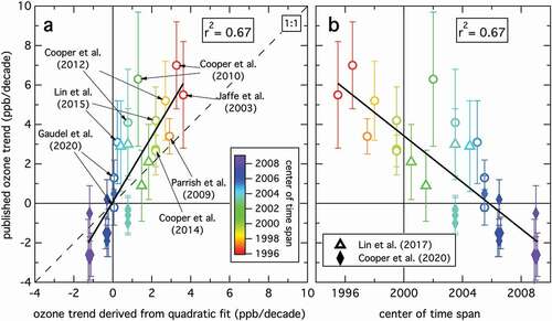
Figure 2. (a) Correlation between published ozone trends (Table 1) and those calculated for the same time periods from the long-term northern mid-latitude baseline ozone change quantified by the quadratic fit for northern mid-latitudes (Parrish et al. 2020). The symbols are color-coded according to the center of the time spans of the data from which the reported trends were derived. The error bars indicate the reported 95% confidence limits of those trends. The linear regression fit and the 1:1 relationship are shown by the solid and dashed lines, respectively; the square of the correlation coefficient is annotated. For clarity, some Cooper et al. (2020) symbols are slightly offset along the x-axis to avoid complete overlap. (b) Correlation between published ozone trends and center of the time spans of the trend determinations. Symbols are in the same format as in (a). Solid line indicates linear regression fit with the square of the correlation coefficient annotated; vertical line indicates t = 0 reference

Within the midlatitude troposphere, the rate of photochemical ozone loss decreases, while the speed of advection increases with altitude (see Supporting Information Section S2 for greater detail). Throughout the bulk of the free troposphere, vertical gradients in baseline ozone arise due to the elevated source in the stratosphere coupled to the surface sink of dry deposition. Modeling of background ozone by Crutzen, Lawrence, and Pöschl (1999) indicates that net photochemical production above about 800 hPa in the northern mid-latitudes ranges from −1.0 ppb/day in the lower troposphere to +0.2 ppb/day in the upper troposphere, further reinforcing the overall positive vertical gradient in baseline ozone, and suggesting a lifetime of ~100 days with respect to net photochemistry throughout the bulk of the troposphere. However, typical convective mass flux schemes suggest that the overturning time scale is between 10 and ~20 days at northern mid-latitudes (Figure S1), which works to reduce the vertical ozone gradient (e.g., Figure 1b, Lelieveld and Crutzen 1994). Overall, the long net ozone lifetime, zonal transport, and relatively rapid vertical overturning imply that a mean ozone concentration is established on a time scale of weeks to months, and that this mean concentration must be similar throughout the northern mid-latitudes; we roughly estimate that this similarity is within ± 10% from ~2 to ~9 km (e.g., see Figure 5 of Parrish et al. 2020). This picture also implies a relatively smooth and systematic seasonal cycle of ozone in baseline air masses.

A zonally similar mean ozone concentration does not imply a lack of ozone variability, as ozone varies about that mean on a wide spectrum of shorter and longer time scales. The mean ozone concentration varies seasonally, due to seasonal changes in sources and sinks. An air parcel within the circulating river of air receives sporadic injections of ozone and its photochemical precursors from European, Asian, and North American anthropogenic sources and from the natural stratospheric source. Ozone injected from the extremely arid stratosphere maintains an anti-correlation with water vapor across vast expanses of the troposphere (Newell et al. 1999) extending its photochemical lifetime with respect to OH production. The infusions of anthropogenic NO_x and VOC precursors into the general tropospheric flow accelerate photochemical ozone production, but also concomitantly enhance photochemical losses as well due to increases in HO_x abundance and production of NO₃ radicals in the dark. Consequently, significant deviations from the circulating mean ozone are brought about in the environment of prolonged net photochemical lifetimes because production and losses tend to be strongly correlated (Figure S2). In addition, air parcels with different ozone production and loss histories are entrained from and exported to higher and lower latitudes. The overall result is local, regional, and quasi-chaotic ozone variability superimposed on the mean concentration. Interannual variability, i.e., changes on time scales of years to ~1 decade, are also important; suggested causes include multi-year climate variability, most prominently the El Niño/Southern Oscillation (ENSO) circulation (e.g., Lin et al. 2014), sporadic events, such as wildfires (Lin et al. 2017), and heatwaves and droughts (Lin et al. 2020).

The subject of this study is decadal and longer scale ozone changes, which are caused by long-term changes in precursor emissions and the changing climate; quantifying these changes must account for the variability of ozone on a wide spectrum of shorter time scales, variability that tends to obscure the long-term changes of interest. Importantly, our guiding conceptual picture implies that these long-term changes must be zonally similar, since it is the zonally similar average ozone concentration that must change; a recent analysis of baseline ozone concentrations on the west coasts of North America and Europe (Parrish et al. 2020) document this expected zonal similarity.

Several terms appear in the literature with reference to the transported ozone concentrations. A common general term is background ozone. However, it is important to note that presently observed concentrations do not represent natural ozone concentrations, i.e., those that existed before industrial development, since anthropogenic emissions of ozone precursors have increased ozone concentrations throughout northern mid-latitudes. For clarity, in this work, we adopt the term “baseline” (e.g., see discussion in Chapter 1 of HTAP 2010) to refer to ozone concentrations measured at locations that receive transported marine air without significant perturbation from recent local or regional North American influences. It is the long-term change in these baseline concentrations that we seek to quantify.

In addition to the linear trend analyses included in Table 1, two published analyses utilized non-linear approaches to quantify long-term changes in baseline ozone concentrations at northern mid-latitudes; both reached similar conclusions. Logan et al. (2012) analyzed several European baseline ozone data sets that extended through 2009, and showed that ozone increased by 6.5–10 ppb in 1978–1989 and 2.5–4.5 ppb in the 1990s, with that increase ending and a maximum reached in the 2000s, followed by decreasing concentrations, at least in summer. Parrish et al. (2020) analyzed those same data sets, which by then extended through 2018, plus additional European and North American data sets; in total 8 baseline data sets from surface sites, balloon-borne sondes and aircraft over Western Europe and western North America were considered. These measurements covered altitudes ranging from sea level to 9 km. Again, an initial, relatively rapid increase was observed, with ozone concentrations reaching a maximum in the mid-2000s, followed by decreasing concentrations. An important conclusion of these analyses is that, within statistical confidence limits, the same non-linear long-term baseline ozone change has occurred throughout the northern mid-latitudes at all altitudes. The goal of this paper is to compare and contrast published linear trend and non-linear long-term change analyses of multi-decadal ozone time series collected at the surface and in the free troposphere over the western US, and to synthesize those analyses to provide an accurate and complete geophysical quantification of long-term changes in baseline ozone on the U.S. West Coast.

Materials and methods

As discussed above, a number of analyses of long-term baseline ozone changes have been published based upon ozone time series collected at a variety of locations in the continental western US. This work is based upon the results of those analyses; no new data sets are analyzed.

Any analysis aiming to quantify the overall long-term change in tropospheric ozone at northern mid-latitudes must effectively deal with two issues: the non-linearity of the long-term changes that have been documented in the previous work, and the substantial interannual variability in mean ozone concentrations that tends to obscure the long-term changes. All linear trend analyses return a single parameter value that quantifies the trend; this is effectively an average slope of the long-term change over the span of the analyzed time series. Hence, due to its very nature, linear trend analysis is ill-suited to quantify non-linear, long-term changes.

We have no a priori knowledge of the functional form of the ozone concentration changes, so long-term change analysis is generally based either on linear trend analyses or on fits of the first few terms of a power series to the time series of measured ozone concentrations. A power series fit does not assume any particular functional form for the time evolution; it is quite flexible, as it can provide a quantitative description of the average continuous, long-term change in any series of observations (Parrish et al. 2019). In practice, the power series fit is obtained through a regression fit of a polynomial to the measurements, with retention of only the statistically significant terms to essure that the time series is not overfit. In this work, no more than the first three terms are considered, as indicated in Equation (1)(1) ${\mathrm{O}}_3=a+bt+c{t}^2,$(1)

(1) ${\mathrm{O}}_3=a+bt+c{t}^2,$(1)

because no more than three statistically significant terms (i.e., those with 95% confidence intervals not containing zero) are encountered in any of the fits to the data sets considered in this study. Section S5 of the Supporting Information more fully discusses power series fits to ozone time series.

Polynomial fits have been used previously to quantify long-term changes in ozone concentrations (e.g., Derwent et al. 2018; Logan et al. 2012; Parrish et al. 2020, 2012; Parrish, Petropavlovskikh, and Oltmans 2017). Importantly, power series fits (including linear fits) are not based on a physical model of the observed temporal changes; consequently, the fitted function cannot be reliably extrapolated to times outside the period of observations; indeed, extrapolation of polynomials (including linear fits) diverges to arbitrarily large positive or negative values at both earlier and later times. The relationship between the quadratic fit used in this analysis and a plausible physical model is discussed in Section S5 of the Supporting Information. Cooper et al. (2020) discuss problems with the use of polynomial fits to characterize long-term ozone changes; the implications of these problems for this work are discussed in Section S6 of the Supporting Information.

Equation (1)(1) ${\mathrm{O}}_3=a+bt+c{t}^2,$(1) does not account for seasonal variations; these variations are eliminated in the studies considered in this work by fitting Equation (1)(1) ${\mathrm{O}}_3=a+bt+c{t}^2,$(1) to annual means, seasonal means, and deseasonalized monthly means (sometimes called monthly residuals or monthly anomalies) to avoid seasonal influences in the data. Ozone concentrations are consistently quantified as mixing ratios, with units of 10⁻⁹ mole O₃ per mole air, denoted as ppb. The time units defined above have been in years, but for ease of presentation and discussion, the quantitative values of the b and c parameters are given in this work as ppb O₃ decade⁻¹ and ppb O₃ decade⁻², respectively.

To precisely determine the coefficients in Equation (1)(1) ${\mathrm{O}}_3=a+bt+c{t}^2,$(1) , the time origin is chosen as the year 2000 (i.e., t in Equation (1)(1) ${\mathrm{O}}_3=a+bt+c{t}^2,$(1) equals the year – 2000) so that the origin falls within the time span of the data series considered. With this choice, the first coefficient (a, with units ppb O₃) is the intercept of the fitted curve at the year 2000; it quantifies the absolute magnitude of the fit to the time series at that year. The second coefficient (b, with units ppb O₃ year⁻¹) is the slope of the fitted curve at that same year; it gives the best estimate of the (continually varying) time rate of change of O₃ in 2000. Finally, the third coefficient (c, with units ppb O₃ year⁻²) gives the constant curvature of the fit, and is equal to one-half of the time rate of change of the slope of the fitted curve. For non-linear time series considered in this work, i.e., those that require fits of Equation (1)(1) ${\mathrm{O}}_3=a+bt+c{t}^2,$(1) with three statistically significant terms, a negative value is consistently derived for c; such fits define curves with ozone concentrations increasing early in the data record, reaching a maximum, and then decreasing at later times. Equation (2)(2) $\mathrm{y}\mathrm{e}\mathrm{a}{\mathrm{r}}_{\mathrm{m}\mathrm{a}\mathrm{x}}=2000-b/2c.$(2) gives the year of the maximum of the fitted curve,

(2) $\mathrm{y}\mathrm{e}\mathrm{a}{\mathrm{r}}_{\mathrm{m}\mathrm{a}\mathrm{x}}=2000-b/2c.$(2)

Parameter values taken from published analyses are generally given with specified 95% confidence limits. We also specify 95% confidence limits in this work. However, it is important to recognize that confidence limits reported in the literature are generally derived from the variability of the data points about the fitted line or curve without a full analysis of the autocorrelation in those data. As a consequence, the quoted confidence limits are generally underestimated to an unknown extent. This issue is important to the present discussion, when comparing and contrasting results from different analyses.

Within the baseline troposphere, average ozone concentrations do exhibit some systematic spatial variability, despite the general zonal uniformity at northern mid-latitudesin particular, baseline ozone concentrations generally increase with altitude (e.g., Oltmans et al. 2008). To compare long-term changes derived from data sets with different mean concentrations, fits of Equation (1)(1) ${\mathrm{O}}_3=a+bt+c{t}^2,$(1) are normalized to zero at the year 2000 by subtracting the corresponding values of the a parameter. The normalization of a linear fit to a quadratic fit is discussed in the following section.

Results and discussion

The results of Parrish et al. (2020) are reproduced in Figure 1a: deseasonalized, normalized monthly means from each of the eight data sets considered (gray points), 2-year averages of those monthly means (black symbols with error bars indicating standard deviations), and a quantification of the average long-term baseline ozone change (black curve). This curve is the least-squares fit of a quadratic polynomial (i.e., Equation (1))(1) ${\mathrm{O}}_3=a+bt+c{t}^2,$(1) to the monthly means. Table 2 gives the parameters of the fit; Equation (2)(2) $\mathrm{y}\mathrm{e}\mathrm{a}{\mathrm{r}}_{\mathrm{m}\mathrm{a}\mathrm{x}}=2000-b/2c.$(2) indicates that a maximum average baseline ozone concentration was reached in the year 2005.7 ± 2.5. Figure 1a also includes quadratic polynomial fits to time series from a US Pacific marine boundary layer (MBL) data set and from one higher altitude (1.8 km) site further inland operated by the National Park Service at Lassen Volcanic National Park. Parrish, Petropavlovskikh, and Oltmans (2017) analyzed these data sets to demonstrate that the long-term trend in baseline ozone concentrations at the US West Coast had reversed from an early increase to a later decrease, with a maximum reached in the early- to the mid-2000s; Figure 1a extends the analysis of those data sets through 2017. These are also two of the eight data sets analyzed by Parrish et al. (2020). There are apparent differences between the three curves, most prominently a more rapid recent decrease in the Pacific MBL data; however, Table 2 shows that the parameters from both the Lassen Volcanic NP and the Pacific MBL fit agree with those of the northern mid-latitude quadratic fit of Parrish et al. (2020) within their indicated confidence limits. Thus, there is no statistically significant difference between the three quadratic fits.

Previously published linear trend analyses of ozone changes within the western US are compared with the results of Parrish et al. (2020) in Figure 1b and Table 1 includes reported trends from 28 separate analyses. Figure 1b represents a selected sample of those trend results by straight-line segments with slopes equal to the reported trends and with lengths equal to the time spans of the analyzed data sets. Each straight-line segment is normalized to the non-linear analysis results by minimizing the sum of the square of the deviations between the line segment and the 2-year averages (black symbols in Figure 1b) that fall within the time span of the corresponding data set. A common general feature characterizes these results – the earlier the start and end times of the trend analysis, the larger the quantified trend. This feature follows from the slowing of the increase in baseline ozone indicated by the black curve in Figure 1. The three earlier analyses (Cooper et al. 2010; Jaffe et al. 2003; Parrish, Millet, and Goldstein 2009) consider data predominately from before the baseline ozone maximum was reached, and therefore report the larger trends. The multiple analyses of Cooper et al. (2020) and the two analyses of Gaudel et al. (2020) cover later time periods that include the ozone maximum with extended periods on either side; they therefore report small trends, some positive and some negative. Cooper et al. (2020) report three analyses, with progressively later starting times for each of 4 data sets; the derived trends become progressively more negative for the later starting times. These features of the linear trend analyses are all consistent with the overall behavior of the quadratic analysis indicated by the black curve.

The 28 referenced trend analyses considered data sets covering a total of 34 years (1984–2017), and derived widely varying trends (−2.8 to +7.0 ppb/decade). The nonlinearity of the long-term change accounts for much of these differences, but interannual variability about the average long-term change also contributes to differences in the results. The analysis of Cooper et al. (2010) gave the largest trend (+7.0 ppb/decade); Lin et al. (2015) show that this result was an overestimate, as were the 5 related analyses included in Cooper et al. (2010, 2012) and Lin et al. (2015), due to substantial influences from interannual variability. None of the 28 trend analysis results accounts for the uncertainties introduced into the results from the autocorrelation in data sets associated with interannual variability (Figure S3), although some address shorter-term, month-to-month autocorrelation (e.g., Gaudel et al. 2020). The analysis based on the non-linear, least-squares fit included in Figure 1 (Parrish et al. 2020) effectively addresses both non-linearity and the longer-term autocorrelation in the longer, 40-year (1978–2017) data set. The resulting quadratic polynomial fit is derived from deseasonalized monthly means, but a fit to the 2-year averages of those monthly means gives nearly identical parameter values, but with significantly larger confidence limits; these larger confidence limits are included in Table 1. The high degree of temporal and spatial averaging in the 2-year means greatly reduces the influence of the autocorrelation associated with interannual variability.

We conclude that the black curve in Figure 1 derived by Parrish et al. (2020) provides a realistic and accurate quantification of the decadal-scale baseline ozone changes over the western US. The results of all published trend analyses are generally consistent with this non-linear fit over the shorter time periods of the trend analyses. The result of each linear trend analysis can be quantitatively compared with the average trend quantified by the quadratic curve over the time period of the trend analysis. The implied trend is derived from the slope of a straight line segment connecting the two points in the quadratic fit at the beginning (t₁) and end (t₂) times of the period included in the trend analysis; this slope is given by

(3) $\mathrm{s}\mathrm{l}\mathrm{o}\mathrm{p}\mathrm{e}=b+c\ast \left({\mathrm{t}}_1+{\mathrm{t}}_2\right).$(3)

Table 1 compares the slopes calculated from Equation (3)(3) $\mathrm{s}\mathrm{l}\mathrm{o}\mathrm{p}\mathrm{e}=b+c\ast \left({\mathrm{t}}_1+{\mathrm{t}}_2\right).$(3) with the published trends, and Figure 2a shows their overall relationship. The non-linear long-term ozone change, as described by the quadratic fit, accounts for ~67% of the variance in the 28 linear trend analysis results. We attribute the remaining ~33% of the variance to the influence of interannual variability, any systematic measurement errors in the multiple data sets analyzed, and any spatial differences between trends at the measurement locations, which include surface sites in marine and continental environments, as well as data sets from the lower and mid-free troposphere. The slope of the standard linear regression (1.65 ± 0.47) included in Figure 2a is greater than unity; we attribute this bias also to the influence of interannual variability. Lin et al. (2015) compare observations with simulations from a global climate model driven by assimilated meteorology; they conclude that meteorologically driven ozone variability has introduced biases into trends derived from observations across the western U.S. In particular, they identify overestimates in the six trends derived by Cooper et al. (2010, 2012) and Lin et al. (2015); these are most of the larger trends reported in the literature, and considered in this work. It is likely that other analyses for this region are affected by this same meteorologically driven variability, so the existing US west coast analyses may overestimate the trends, consistent with the conclusions of Lin et al. (2015) and the slope of the regression line in Figure 2a. Systematic measurement errors and spatial differences may possibly contribute to the unexplained variability, but we have found no evidence for a contribution from either. Parrish et al. (2020) conclude that there are no statistically significant differences in the long‐term baseline ozone changes within the lower troposphere at northern midlatitudes, so a contribution from spatial differences is not expected.

It is possible to independently determine a quadratic description of the overall long-term ozone changes from the reported linear trends. Equation (3)(3) $\mathrm{s}\mathrm{l}\mathrm{o}\mathrm{p}\mathrm{e}=b+c\ast \left({\mathrm{t}}_1+{\mathrm{t}}_2\right).$(3) indicates that a plot of the derived trends as a function of the centers of the time periods of the respective trend determinations will define a straight line with a slope of 2*c and a y-intercept of b, where c and b are the parameters of a quadratic curve as given by Equation (1)(1) ${\mathrm{O}}_3=a+bt+c{t}^2,$(1) . Figure 2b shows that plot, which includes a linear regression to the 28 trend determinations. Note that the x–intercept corresponds to the time when the trend is zero, which is thus the year_max given by Equation (2)(2) $\mathrm{y}\mathrm{e}\mathrm{a}{\mathrm{r}}_{\mathrm{m}\mathrm{a}\mathrm{x}}=2000-b/2c.$(2) . Table 2 compares the parameters from this quadratic determination with the three discussed previously; generally, there is agreement within the indicated confidence limits, but reasons for exceptions to this agreement are discussed below.

The error bars illustrated in Figure 2a indicate the 95% confidence limits reported for the respective trends. Assuming 1) that there are no systematic errors in any of the analyses and 2) that the confidence limits are accurately quantified, it is expected that only ~5% of the error bars in Figure 2a would fail to overlap with the 1:1 line; however, the actual fraction is 57%. (Table 1 includes confidence limits for the slopes derived from the quadratic curve through a propagation of error calculation based on the confidence limits of the quadratic parameters indicated in Table 2; substitution of these confidence limits in Figure 2a would not significantly increase the number of points overlapping the 1:1 line.) Similarly, only 64% of the parameter values compared in Table 1 agree within the derived 95% confidence limits. There is a clear lack of consistent agreement within the 95% confidence limits between trend values reported in the literature and those derived from the quadratic fit; we attribute this lack of agreement primarily to underestimation of the confidence limits in the trend analyses reported in the literature, and this underestimation is due to inadequate treatment of the autocorrelation in the data sets resulting from interannual variability. The trends derived in the six earlier analyses of springtime ozone mixing ratios in the free troposphere over western North America (Cooper et al. 2012, 2010; Lin et al. 2015) are particularly influenced by interannual variability; as discussed by Lin et al. (2015) interannual variability, as well as sampling bias in some of the aircraft data sets, led to overestimates of the derived trends by a factor of ~2.

To approximately quantify the influence of autocorrelation on the confidence limits reported for the literature trends included in Table 1 and indicated by the error bars in Figure 2, we consider the effect of an arbitrary 50% increase in those confidence limits. This increase brings the fraction of confidence limits overlapping the 1:1 line into close agreement with the expected 95%, and eliminates the disagreements in Table 2. This result suggests that autocorrelation, not considered in the published analyses, reduced the number of independent data points in the analyzed data sets by a factor of ~2 on average. The scatter of the trend analyses of the fits in Figure 2 emphasizes the importance of careful consideration of the impact of autocorrelation arising from interannual variability in the quantification of long-term changes on the basis of time series of ozone measurements.

Summary and conclusion

The long net lifetime of ozone in the prevailing westerly winds at northern mid-latitudes implies that a common long-term change in mean baseline ozone concentrations must have occurred throughout this zone. Parrish et al. (2020) document this similarity and quantify the long-term change with a fit of a quadratic polynomial to monthly and biennial means of multiple data sets. Linear trends reported for different time periods in 28 published analyses of western US baseline ozone data sets vary between −2.8 and +7.0 ppb/decade. The quadratic fit of Parrish et al. (2020) accounts for about two-thirds of the variance in the trend results, with the remaining one-third of the variance attributed to interannual variability that adds uncertainty to the trend determinations. All reported trend analyses for western US baseline ozone data sets are consistent with the picture conveyed by that quadratic fit – ozone increasing rapidly (~5 ppb/decade) at the beginning of measurement records with that increase progressively slowing, and ozone reaching a maximum in the mid-2000s and decreasing slowly (~1 ppb/decade) thereafter. The quadratic fit provides an excellent fit to the twenty 2-year means over the 1978–2017 period, capturing about 89% of their variance with a root-mean-square deviation between the fit and the means of 1.3 ppb.

Baseline ozone transported into the U.S. constitutes a large fraction of the 70 ppb ozone National Ambient Air Quality Standard (NAAQS). The mixing ratio of background ozone in air entering the west coast of the US has been measured by sondes launched from Trinidad Head on the northern California coast (Oltmans et al. 2008); the concentration at 1 km altitude averaged 42 ppb from 1997 to 2014 with a standard deviation of 12 ppb. These observations are in accord with the US EPA policy assessment conducted for the recent review of the ozone National Ambient Air Quality Standard (NAAQS) which found that regional average MDA8 ozone concentrations in the western US maximized in summer 2016 at ~52 ppb and that ~40 ppb of that maximum was contributed by ozone of natural and transported anthropogenic contributions (Figures 2–23 of US EPA, 2020). Thus, changes in baseline ozone concentrations affect the difficulty of achieving the NAAQS in US nonattainment areas. Between 1980s and 1990s, those baseline concentrations were increasing, making attainment of U.S. air quality goals progressively more difficult and partially offsetting the air quality improvement that resulted from emission controls (Jacob, Logan, and Murti 1999). In the mid-2000s baseline ozone concentrations maximized and then slowly decreased at an average rate of 0.9 ± 0.8 ppb decade⁻¹ over the 2000–2018 period (Parrish et al. 2020). This small decrease, if continued, would gradually lessen the difficulty of achieving US air quality goals. However, despite the changes evident in Figure 1, average baseline ozone concentrations entering the western US have remained within a narrow range over the 1990–2017 period; the standard deviation of the fourteen 2-year means is only 1.5 ppb. Improvement in US ozone air quality has come primarily from continued precursor emission controls that reduce local and regional photochemical ozone production; this improvement can continue and possibly be augmented by international efforts to reduce anthropogenic precursor emissions from all sources at northern mid-latitudes, thereby reducing the hemisphere-wide transported baseline ozone concentrations.

Key points

• Reported trends in tropospheric ozone concentrations transported into the Western US vary between −2.8 and +7.0 ppb/decade

• All reported trends agree with an overall non-linear change – ozone increasing before the mid-2000s and slowly decreasing thereafter

• About 1/3 of the variance in reported trends is due to autocorrelation in the data, which was not adequately considered in prior analyses

Acknowledgment

The authors are grateful for the extensive ozone trend analyses that have been published in the scientific literature; all results on which this paper is based are reported in the cited references. The efforts of I.C.F. were supported by the California Agricultural Experiment Station Hatch Project CA-D-LAW-2481-H. Support for the Twentieth Century Reanalysis Project dataset is provided by the U.S. Department of Energy, Office of Science Innovative and Novel Computational Impact on Theory and Experiment (DOE INCITE) program, and Office of Biological and Environmental Research (BER), and by the National Oceanic and Atmospheric Administration Climate Program Office. The authors have no conflicts of interests.

Disclosure statement

No potential conflict of interest was reported by the author(s).

Supplementary material

Supplemental data for this paper can be accessed on the publisher’s website.

Additional information

Notes on contributors

David D. Parrish

David D. Parrish is an atmospheric chemist who now focuses on tropospheric ozone analyses. He has worked in atmospheric research in Boulder Colorado for more than forty years, and currently is an independent scientist and consultant at David.D.Parrish, LLC.

Richard G. Derwent

Richard G. Derwent is an independent scientist and consultant on air pollution and atmospheric chemistry with rdscientific, Newbury, United Kingdom.

Ian C. Faloona

Ian C. Faloona is a professor of atmospheric science at the University of California Davis, and a Bio-micrometeorologist with the Agricultural Experiment Station. He studied physical chemistry at the University of California Santa Cruz, spent 5 years as an air quality consultant with SECOR, Inc. in Fort Collins, Colorado, and then earned a Ph.D. in Meteorology at the Pennsylvania State University.  His research interests include the airborne investigation of vertical mixing and near-field pollutant dispersion, observational emission estimates,  planetary boundary layer dynamics, biogeochemical cycling, and atmosphere/ocean photochemistry.

References

- Collins, W. J., D. S. Stevenson, C. E. Johnson, and R. G. Derwent. 1997. Tropospheric ozone in a global-scale three-dimensional Lagrangian model and its response to NOx emission controls. J. Atmos. Chem. 26:223–74. doi:https://doi.org/10.1023/A:1005836531979.
- Cooper, O. R., R.-S. Gao, D. Tarasick, T. Leblanc, and C. Sweeney. 2012. Long-term ozone trends at rural ozone monitoring sites across the United States, 1990–2010. J. Geophys. Res. 117:D22307. doi:https://doi.org/10.1029/2012JD018261.
- Cooper, O. R., D. D. Parrish, A. Stohl, M. Trainer, P. Nédélec, V. Thouret, J. P. Cammas, S. J. Oltmans, B. J. Johnson, D. Tarasick, et al. 2010. Increasing springtime ozone mixing ratios in the free troposphere over western North America. Nature 463 (7279):344–48. doi:https://doi.org/10.1038/nature08708.
- Cooper, O. R., D. D. Parrish, J. Ziemke, N. V. Balashov, M. Cupeiro, I. E. Galbally, S. Gilge, L. Horowitz, N. R. Jensen, J.-F. Lamarque, et al. 2014. Global distribution and trends of tropospheric ozone: An observation-based review. Elem. Sci. Anth. 2:29. doi:https://doi.org/10.12952/journal.elementa.000029.
- Cooper, O. R., M. G. Schultz, S. Schröder, K.-L. Chang, A. Gaudel, G. C. Benítez, E. Cuevas, M. Fröhlich, I. E. Galbally, S. Molloy, et al. 2020. Multi-decadal surface ozone trends at globally distributed remote locations. Elem. Sci. Anth. 8:23. doi:https://doi.org/10.1525/elementa.420.
- Crutzen, P. J., M. G. Lawrence, and U. Pöschl. 1999. On the background photochemistry of tropospheric ozone. Tellus B 51 (1):123–46. doi:https://doi.org/10.3402/tellusb.v51i1.16264.
- Derwent, R. G., D. D. Parrish, I. E. Galbally, D. S. Stevenson, R. M. Doherty, V. Naik, and P. J. Young. 2018. Uncertainties in models of tropospheric ozone based on Monte Carlo analysis: Tropospheric ozone burdens, atmospheric lifetimes and surface distributions. Atmos. Environ. 180:93–102. doi:https://doi.org/10.1016/j.atmosenv.2018.02.047.
- Gaudel, A., O. R. Cooper, K.-L. Chang, I. Bourgeois, J. R. Ziemke, S. A. Strode, L. D. Oman, P. Sellitto, P. Nédélec, R. Blot, et al. 2020. Aircraft observations since the 1990s reveal increases of tropospheric ozone at multiple locations across the Northern Hemisphere. Sci. Adv. 6 (34):eaba8272. doi:https://doi.org/10.1126/sciadv.aba8272.
- HTAP. 2010. Hemispheric transport of air pollution 2010, part A: Ozone and particulate matter, air pollution studies no. 17. Edited by F. Dentener, T. Keating T, and H. Akimoto. New York and Geneva: United Nations.
- Jacob, D. J., J. A. Logan, and P. P. Murti. 1999. Effect of rising Asian emissions on surface ozone in the United States. Geophys. Res. Lett. 26:2175–78. doi:https://doi.org/10.1029/1999GL900450.
- Jaffe, D., H. Price, D. D. Parrish, A. Goldstein, and J. Harris. 2003. Increasing background ozone during spring on the west coast of North America. Geophys. Res. Lett. 30 (12):1613. doi:https://doi.org/10.1029/2003GL017024.
- Lelieveld, J., and P. J. Crutzen. 1994. Role of deep cloud convection in the ozone budget of the troposphere. Science 264 (5166):1759–61. doi:https://doi.org/10.1126/science.264.5166.1759.
- Lin, M., L. W. Horowitz, O. R. Cooper, D. Tarasick, S. Conley, L. T. Iraci, B. Johnson, T. Leblanc, I. Petropavlovskikh, and E. L. Yates. 2015. Revisiting the evidence of increasing springtime ozone mixing ratios in the free troposphere over western North America. Geophys. Res. Lett. 42 (20):8719–28. doi:https://doi.org/10.1002/2015GL065311.
- Lin, M., L. W. Horowitz, S. J. Oltmans, A. M. Fiore, and S. Fan. 2014. Tropospheric ozone trends at Mauna Loa observatory tied to decadal climate variability. Nat. Geosci. 7 (2):136–43. doi:https://doi.org/10.1038/ngeo2066.
- Lin, M., L. W. Horowitz, S. J. Oltmans, A. M. Fiore, and S. Fan. 2017. US surface ozone trends and extremes from 1980 to 2014: Quantifying the roles of rising Asian emissions, domestic controls, wildfires, and climate. Atmos. Chem. Phys. 17:2943–70. doi:https://doi.org/10.5194/acp-17-2943-2017.
- Lin, M., L. W. Horowitz, Y. Xie, F. Paulot, S. Malyshev, E. Shevliakova, A. Finco, G. Gerosa, D. Kubistin, K. Pilegaard, et al. 2020. Vegetation feedbacks during drought exacerbate ozone air pollution extremes in Europe. Nat. Clim. Chang. 10 (5):444–51. doi:https://doi.org/10.1038/s41558-020-0743-y.
- Logan, J. A., J. Staehelin, I. A. Megretskaia, J. ‐. P. Cammas, V. Thouret, H. Claude, H. De Backer, M. Steinbacher, H.-E. Scheel, R. Stübi, et al. 2012. Changes in ozone over Europe: Analysis of ozone measurements from sondes, regular aircraft (MOZAIC) and alpine surface sites. J. Geophys. Res. 117:D09301. doi:https://doi.org/10.1029/2011JD016952.
- Newell, R. E., V. Thouret, J. Y. N. Cho, P. Stoller, A. Marenco, and H. G. Smit. 1999. Ubiquity of quasi-horizontal layers in the troposphere. Nature 398 (6725):316–19. doi:https://doi.org/10.1038/18642.
- Oltmans, S. J., A. S. Lefohn, J. M. Harris, and D. S. Shadwick. 2008. Background ozone levels of air entering the west coast of the U.S. and assessment of longer-term changes. Atmos. Environ. 42:6020–38. doi:https://doi.org/10.1016/j.atmosenv.2008.03.034.
- Parrish, D. D., R. G. Derwent, S. O’Doherty, and P. G. Simmonds. 2019. Flexible approach for quantifying average long-term changes and seasonal cycles of tropospheric trace species. Atmos. Meas. Tech. 12:3383–94. doi:https://doi.org/10.5194/amt-12-3383-2019.
- Parrish, D. D., R. G. Derwent, W. Steinbrecht, R. Stübi, R. Van Malderen, M. Steinbacher, T. Trickl, L. Ries, and X. Xu. 2020. Zonal similarity of long-term changes and seasonal cycles of baseline ozone at northern mid-latitudes. J. Geophys. Res. doi:https://doi.org/10.1029/2019JD031908.
- Parrish, D. D., K. S. Law, J. Staehelin, R. Derwent, O. R. Cooper, H. Tanimoto, A. Volz-Thomas, S. Gilge, H.-E. Scheel, M. Steinbacher, et al. 2012. Long‐term changes in lower tropospheric baseline ozone concentrations at northern mid‐latitudes. Atmos. Chem. Phys. 12 (11):485–11,504. doi:https://doi.org/10.5194/acp-12-11485-2012.
- Parrish, D. D., D. B. Millet, and A. H. Goldstein. 2009. Increasing ozone in marine boundary layer air inflow at the west coasts of North America and Europe. Atmos. Chem. Phys. 9:1303–23. doi:https://doi.org/10.5194/acp-9-1303-2009.
- Parrish, D. D., I. Petropavlovskikh, and S. J. Oltmans. 2017. Reversal of long-term trend in baseline ozone concentrations at the North American West Coast. Geophys. Res. Lett. 44. doi:https://doi.org/10.1002/2017GL074960.
- Peixoto, J. P., and A. H. Oort. 1992. Physics of climate. New York, NY: American Inst. of Physics.
- U.S. EPA. May 2020. Policy assessment for the review of the ozone national ambient air quality standards. EPA. EPA-452/R-20-001, Office of Air Quality Planning and Standards, Health and Environmental Impacts Division. Research Triangle Park, NC. https://www.epa.gov/sites/production/files/2020-05/documents/o3-final_pa-05-29-20compressed.pdf.