Zero-impact emission limits of enterprise-scale air pollutants—a case study of a typical petrochemical enterprise in Shanghai Chemical Industry Park

ABSTRACT

The implementation of pollutant emission control has made initial achievements in the plant power, iron, and steel industries in China. To further improve air quality, it is of great significance to carry out research on zero-impact emissions of the petrochemical industry. Based on the existing concept and practice of zero emissions, this study proposes the concept of zero-impact emissions, taking emission concentration as the constraint. A typical petrochemical enterprise (namely Enterprise A) in Shanghai Chemical Industry Park as the research object, and used the CALPUFF model to simulate the target pollutant emissions (i.e. sulfur dioxide (SO₂), nitrogen oxide (NO_x), particulate matter (PM), and volatile organic compounds (VOCs)). The current emission standard, spatial distributions, and emission heights of chimneys in Enterprise A was considered as the baseline emission scenario and taking the zero-impact emission as a target for simulation. The results show that the current emission standards of NO_x and VOCs (benzene) exceeded the zero-impact emission limits, and needed to be reduced by 22% and 87.5%, respectively. Moreover, the areas that exceeded the zero-impact concentration limits were located northwest of the chimneys and Hangzhou Bay. In terms of seasonal effects, the wind conditions in spring were more adverse for the enterprise to achieve zero-impact emissions. Based on the simulation, the zero-impact emission limits of SO₂, NO_x, PM, and VOCs (benzene) for Enterprise A were 50 mg/m³, 78 mg/m³, 10 mg/m³, and 0.32 mg/m³, respectively.

Implications: Through case study, this paper solves the environmental management issue which is of universal significance for chemical industry park. The concept of zero-impact emissions and the determination method of zero-impact concentration limits proposed in this study could be used as references for related research on cutting emissions. Although the conclusion of this study about the emission limits is not suitable for other enterprises to apply directly, the calculation method of zero-impact emission limit can be used by other enterprises. Furthermore, the zero-impact emission limits on park scale can be determined after comprehensive evaluation based on the calculation results of multiple enterprises.

Introduction

The zero-emissions concept was first proposed in the 1990s. In 1994, the United Nations University (UNU), headquartered in Tokyo, launched a zero-emissions project based on research and action (Kuehr 2000; Suzuki 2000). Zero emissions include activities that minimize pollutant emissions and energy consumption to zero.

The plan to establish Zero Emissions Industrial Parks (https://www.meti.go.jp/policy/recycle/main/3r_policy/policy/ecotown.html) was put forward by the Japanese government in 1997, which was the first implementation of combining industrial parks with the concept of zero emissions. In the idea, the park is designed as an integrated network composed of different enterprises. All types of waste discharged are traded among the enterprises within the park to realize large-scale treatment and minimize costs, and ultimately achieve zero emissions. Japan’s zero-emission industrial parks are essentially closer to eco-industrial parks, which are widely present in the world (United Nations Environment Programme [UNEP] 1997). In these parks, pollutant emission control is generally implemented by improving the utilization efficiency of resources and energy to critically control the total amount of regional waste emissions.

When Germany accepted the zero-emissions concept, they put forward the Joint Zero Emission Innovation Project, and developed the GaBi software combined with life cycle assessment technology. The GaBi software realizes quantitative and qualitative analysis of logistics and energy consumption during the production process, and provides potential improvements to the existing zero-emission system (Liang et al. 2020; Matsuno et al. 2013; Yang et al. 2019). Hence, the zero-emission concept is no longer within industrial parks, but extends beyond boundaries to more fields and larger regions.

Currently, zero emissions involve many sectors (e.g., construction, motor, industry). In the industrial sector, many countries have been working to achieve zero air pollutant emissions during the production process. Yantovski et al. (2004) described a zero-emission, gas-fired power plant for electricity generation, in which all the combustion products were in liquid and not gaseous form. The problem of zero emissions translated into the conversion of emissions to effluents. Krajnc, Mele, and Glavič (2007) discussed the possibility of attaining zero emissions in the case of sugar production and suggested that changing the fuel type used in the sugar plant (replacement of heavy fuel oil with natural gas) produced a significant decrease in air emissions. Zhou et al. (2015) and Wang et al. (2018) studied the near-zero emissions of coal-fired power plants. These studies focused on emission mitigation technologies (e.g., desulfurization, denitration, and dust removal technology) and their industrial applications.

However, considering thermodynamic processes, zero emissions are theoretically impossible to achieve. For example, in a chemical reaction, it is unrealistic to reach a 100% yield rate, where waste heat emissions are inevitable (Kuehr 2007). Therefore, the expressions of near-zero and net-zero emissions are more common in current research and practice (Kaufman et al. 2020; Levy 2013; Matthews and Caldeira 2008; Sproul, Barlow, and Quinn 2020; Wang et al. 2015). Furthermore, for an enterprise, emissions reduction relies heavily on various mitigation techniques (Brown et al. 2021; Cao, Garbaccio, and Ho 2009; Lee and Cho 2003), which are always significantly costly (Zhao, Jin, and Zhang 2016).

Implementing ultra-low emission standards, which are the closest pollution control practices to zero emissions, China has made remarkable achievements in reducing industrial air pollutants from the energy, iron, steel, and other industries (Jiao et al. 2020; Tang et al. 2020; Wang et al. 2015; Xia et al. 2020; Yang et al. 2018; Zhang et al. 2015). China’s ultra-low emission (ULE) standards (particulate matter (PM), SO₂, and NO_x emissions are limited to 10 mg/m³, 35 mg/m³, and 50 mg/m³, respectively) as set in the Action Plan for Energy Conservation and Emission Reduction Upgrading and Transformation of Coal Power (2014–2020) (www.gov.cn/zwgk/2013-09/12/content_2486773.htm), based on the technical route for concentration control, with the goal of satisfying the Level 2 standard of the Chinese National Ambient Air Quality Standard (GB3095-2012). By 2017, China’s power plant industry had successfully achieved ultra-low emission transformation targets, and the emissions of PM, SO₂, and NO_x decreased by more than 60% (Tang et al. 2019). Moreover, China’s ultra-low emission practice has also been gradually implemented in the iron and steel industry. Compared with 2017, the total NO_x, SO₂, and PM emissions from iron and steel enterprises in 2018 were reduced by 7%, 6%, and 28%, respectively (Zhang et al. 2020).

Despite the rewarding transformation of ultra-low emissions, China’s air pollution is still serious, which poses a risk to public health (Biswas, Chatterjee, and Chakraborty 2020; Cui et al. 2021; Fan, Zhao, and Yang 2020; Filonchyk and Yan 2018; Huang, Yan, and Zhang 2018; Li et al., 2019a, 2019b; Liu et al. 2018; Tian et al. 2020; Wang et al. 2020). Air pollutant emissions should be further reduced as far as possible. Furthermore, the petrochemical industry is currently one of the major sources of air pollution compared to that of other industries (Zheng et al. 2018). It consumes a large amount of fossil energy such as oil and coal, and produces and emits a large number of pollutants throughout its technological and fuel combustion process, which have a disastrous impact on air quality (Jia et al. 2020; Li et al. 2020; Lin, Lai, and Chu 2021; Zheng et al. 2020). However, previous research on cutting emissions focused on the application of clean fuels and the exploration of emission reduction technologies, and relatively few studies have focused on emission limits. Therefore, it is of great significance to study zero-impact emission limits in the petrochemical industry.

Due to the influence of technology and environmental protection policies, there are great differences in the air pollutant emission standards of the petrochemical industry worldwide (Table 1). As shown in Table 1, China’s emission standards for the petrochemical industry are relatively stringent. Shanghai Chemical Industrial Park (SCIP) is an advanced industrial park that mainly focuses on petrochemical products, with strict safety and environmental protection management and a high level of circular economy. Synthetically comparing the emission standards of the above regions, the SCIP formulated unified emission standards that are stricter than the emission standards of pollutants for the petroleum chemistry industry in China (GB 31571–2015) in 2016.

Table 1. Air pollutant emission standards of the petrochemical industry worldwide. (unit: mg/m³)

Pollutants	Nitrogen oxide (NOx)	Sulfur dioxide (SO2)	Particulate matter (PM)	VOCs
				(benzene)
Industrial Emissions Directive in EU (2010/75/EU)	50 ~ 100	50	10	1
Emission standard of pollutants for petroleum chemistry industry in China (GB 31571–2015)	100	50	20	4
Technical instructions for air purification in Germany (TA Luft 2002)	200	60	20 ~ 50	1
Pollution Prevention and Abatement Hand Book by World Bank	300	100	20	1
Emission standard of pollutants in Shanghai Chemical Industry Park	100	50	10	4

Taking a typical petrochemical enterprise (Enterprise A) in Shanghai Chemical Industry Park (SCIP) as an example, this study examines the zero-impact emissions of petrochemical enterprises based on the technical route of concentration control. The concept of zero-impact emissions proposed in this study is different from zero emissions or ultra-low emissions in previous studies at the park and industry levels, and the determination of the emission limit is innovatively combined with the numerical model. In Section 2, we first introduce the study case, including information on Enterprise A and its baseline emission scenario, as well as the meteorological and air quality conditions in the study area. In Section 3, we introduce the concept of zero-impact emissions, determine the zero-impact concentration limits, and introduce the calculation method for zero-impact emission limits. Section 4 compares the ground-level concentration of pollutants with zero-impact concentration limits, calculates the zero-impact emission limits, and analyzes the zero-impact emission limit to determine whether it can be achieved in a shorter average time. Section 5 discusses the recommendations for future research, followed by the conclusions in Section 6.

Case study

Introduction of Enterprise A and baseline emission scenario

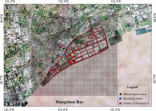
Enterprise A is located in the SCIP, on the North Bank of Hangzhou Bay, covering an area of approximately 2 km². The enterprise mainly produces ethylene, propylene, polyethylene, benzene, toluene, and by-products, with an annual output of 3.2 million tons of petrochemical products. The enterprise has 22 chimneys (Figure 1), and the chimneys discharge NO_x, SO₂, PM, and VOCs as main pollutants. Table 2 provides basic information on each chimney based on field research, environmental impact assessment (EIA) report of Enterprise A, and the emission information platform of Shanghai enterprises and institutions (https://xxgk.eic.sh.cn/jsp/view/index.jsp).

Table 2. Basic information of each chimney of Enterprise A

No.	Chimney height(m)	Chimney diameter(m)	Pollutant
1	50	2.48	NOx\PM\VOCs
2	50	2.48	NOx\PM\VOCs
3	50	2.48	NOx\PM\VOCs
4	50	2.5	NOx\PM\VOCs
5	50	2.56	NOx\PM\VOCs
6	50	2.5	NOx\PM\VOCs
7	50	2.48	NOx\PM\VOCs
8	50	2.48	NOx\PM\VOCs
9	50	2.48	NOx\PM\VOCs
10	50	2.58	NOx\PM\VOCs
11	50	2.58	NOx\PM\VOCs
12	15	1.25	NOx\SO2\PM\VOCs
13	15	0.75	NOx\SO2\PM\VOCs
14	24	0.3	NOx\SO2
15	65	2.8	NOx\SO2\VOCs
16	65	2.37	NOx\SO2\VOCs
17	65	2.37	NOx\SO2\VOCs
18	50	2.8	NOx\VOCs
19	50	1.5	NOx\SO2\PM\VOCs
20	80	4.8	NOx\SO2\VOCs
21	80	1.5	NOx\SO2\PM\VOCs
22	68	3.3	NOx\SO2

Figure 1. Distribution of chimneys, and meteorological and monitoring stations

In this study, the baseline emission scenario refers to the emissions of Enterprise A according to the current emission standards (Table 1), under the existing chimney height, diameter (Table 2), and distribution. For VOCs, the baseline emission scenario also involves the fugitive emissions, and the total fugitive emission of benzene from Enterprise A is 143.33 ton in 2019 (EIA report of Enterprise A).

Moreover, the simulations were carried out under a clean background, hence the pollutant concentration obtained was the net increase caused by Enterprise A.

Meteorological and air quality conditions

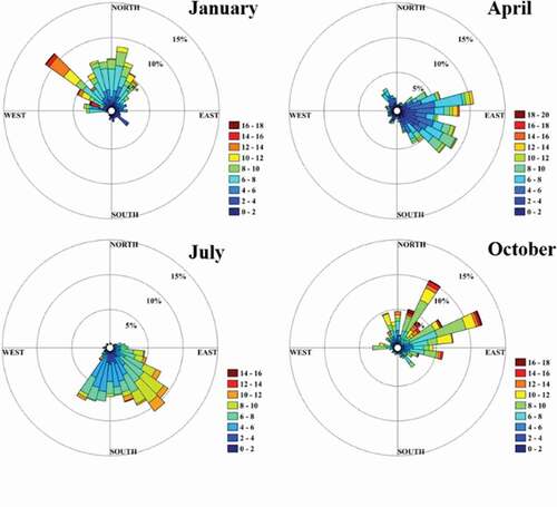
Shanghai Chemical Industrial Park is located at the junction of the continent and sea on the north coast of Hangzhou Bay, which is affected by the mainland and ocean air mass. Under the influence of the land-sea thermal properties in different seasons, the dominant wind direction of this park has a remarkable seasonal variation. According to the characteristics of the wind field in each season, January, April, July, and October can be the representative months typical of the four seasons.

As shown in the monthly wind increase in the SCIP in 2019 (Figure 2), which is based on the wind direction and speed data of the meteorological station in Figure 1, the dominant wind direction in January is northwesterly and northerly, with a combined frequency of the two directions of 61.34%, and the average wind speed of 6.62 m/s. The dominant wind direction in April is easterly (45.49%), and the average wind speed is 5.78 m/s. In July, the dominant wind direction is southeasterly and southerly, with a combined frequency of 71.31% and an average wind speed of 6.29 m/s. In October, the dominant wind direction is northeasterly and easterly, with a combined frequency of 58.52% and an average wind speed of 8.09 m/s. The annual frequency of the west wind is the lowest (5.06%), with an average annual wind speed of approximately 6.7 m/s.

Figure 2. Wind roses in January, April, July, and October in Shanghai Chemical Industry Park (SCIP) in 2019

Air quality is greatly affected by the emissions from production activities in the region. According to the pollutant concentration data measured at the monitoring station near Enterprise A in Figure 1, the average annual concentrations of conventional pollutants PM₁₀, PM_2.5, SO₂, and NO_x in 2019 are 47.25 µg/m³, 35.21 µm/m³, 9.25 µg/m³, and 49.22 µg/m³, respectively. The maximum 1-hour concentration of VOCs (benzene) is 45.56 µg/m³.

Methodology

Considering the technical and economic feasibility, taking the principle of sustainable development, the concept of zero-impact emissions is defined at the enterprise level with a concentration constraint. In this sense, the study of zero-impact emission in this study needs to first define two limits: zero-impact concentration limits and zero-impact emission limits. After emission, the air pollutants are diluted and diffused, and these emissions are defined as zero-impact emissions if the final concentration at a certain control area meets the zero-impact concentration limit. In actual research, there are two constraints on the control area of zero-impact concentration limits, one is the boundary concentration constraint (i.e., with the maximum ground level concentration within the factory boundary not greater than that of the zero-impact concentration limit), and the maximum ground-level concentration constraint (i.e., with the maximum ground level concentration in the control area not greater than that of the zero-impact concentration limit). If the maximum ground-level concentration meets the above two constraints, the emission will not have an adverse impact on the environmental quality or health effects in areas, that is, zero-impact emissions will be achieved.

In this study, the time scales of zero-impact concentration limits were determined by referring to the traditional practice of air quality management in China. For conventional pollutants such as SO₂, NO_x, and PM, their long-term impacts were considered, and their zero-impact concentration limits were determined on an annual average scale. At the same time, analysis of the 24- and 1-hour average concentrations was also carried out even when it was not used for the constraint of emission limits. According to the analysis of the particle size distribution of PM emission in the actual monitoring of petrochemical enterprises, the PM exhausted from Enterprise A was approximately all regarded as PM₁₀, whereas PM_2.5 accounted for 65% of PM₁₀ (Ehrlich et al. 2007). For VOCs, we only considered its short-term impact and determined its hourly zero-impact concentration limit.

In addition, we defined zero-impact emission limits specific to the concentrations of chimney pollutants. During production activities, if the maximum ground-level concentration of the pollutant reaches the zero-impact concentration limit, the emission concentration at that time is the zero-impact emission limit.

Determination of zero-impact concentration limits

Currently, China’s environmental protection requirements and policies aim to reach Level II of the Chinese National Ambient Air Quality Standard. However, there is still a gap between Level II standards of air pollutants in China and those recommended by the World Health Organization (WHO). Considering that the air quality of most cities in China (46.6%) has reached Level II standards, and the ultra-low emission of plant power, iron, steel, and other industries has been mostly realized, as required by the increasingly stringent emission reduction requirements of China, this study takes the Level I standard of the Chinese National Ambient Air Quality Standard as the reference value to determine the zero-impact concentration limits.

However, defining the impact extent of an enterprise’s pollutant emissions was the key problem to be solved in this study. When carrying out environmental impact assessments in China, the maximum distance corresponding to the pollutant ground-level concentration satisfying 10% of the Level II standard is usually taken as the reference to determine the scope of environmental impact assessment (HJ 2.2–2018). In other words, when the concentration of a pollutant is higher than 10% of Level II standards, the pollutant is considered to have an impact on the environmental quality of a specific object or area. Otherwise, it can be considered a zero impact.

Considering the current situation of China’s environmental protection, Chinese air quality standards, and the approach to identify the impact scope in environmental impact assessment, this study determined 10% of the Level I standard of each pollutant on the annual average scale in the Chinese National Ambient Air Quality Standard (GB3095-2012) as the zero-impact concentration limits. At the same time, 10% of the Level I standard of each conventional pollutant on the 24-hour and 1-hour average time scales were regarded as the reference concentration of zero-impact emissions. The equation for the zero-impact concentration limits of conventional pollutants is as follows:

(1) $L_c=Con\times 10\mathrm{\%}$(1)

where $L_c$ is the zero-impact concentration limit of each conventional pollutant, and $Con$ is the Level I standard of each pollutant on the annual average scale in the Chinese National Ambient Air Quality Standard.

In addition to conventional pollutants, VOCs were also included in this study as a key pollutant according to the emission characteristics of petrochemical enterprises. In terms of VOC emission control, the U.S. Environmental Protection Agency (U.S. EPA) has developed a relatively systematic and accomplished emission standard, and set a concentration limit of 9 µg/m³ for benzene at the factory boundary (U.S. EPA 2015). According to this limit, the zero-impact concentration limit of VOCs (benzene) was set to 9 µg/m³ in this study.

According to the different average times of air quality standard for the annual, 24-hour, and 1-hour, this study provides the zero-impact concentration limits of conventional pollutants SO₂, NO_x, PM₁₀, and CO in their corresponding average times. For VOCs, we considered the zero-impact concentration limit among the 1-hour average time. The zero-impact concentration limits for each pollutant are listed in Table 3.

Table 3. Zero-impact concentration limits of each pollutant and 10% concentration of conventional pollutants as short-term average time

No.	Pollutants	Average time	concentration
			($\mu \mathbf{g}/m^3$)
1	SO2	Annual	2*
		24-hour	5**
		1-hour	15**
2	NOx	Annual	5*
		24-hour	10**
		1-hour	25**
3	PM10 (Particle diameter ≤ 10 µm)	Annual	4*
		24-hour	5**
4	PM2.5 (Particle diameter ≤ 2.5 µm)	Annual	1.5*
		24-hour	3.5**
5	VOCs (benzene)	1-hour	9*

*is the zero-impact concentration limit, and * * is the 10% concentration of the Level I standard of each pollutant on the 24-hour and 1-hour average time scales.

Calculation scheme of zero-impact emission limits

In this study, four typical meteorological fields in January, April, July, and October 2019 were selected as the background, and the California Puff (CALPUFF) model was used to simulate the transmission and diffusion of air pollutants from Enterprise A under the baseline emission scenario, which was introduced in Section 2.1. The zero-impact emission limit of each chimney was deduced by comparing the maximum ground concentration of each pollutant with its zero-impact concentration limit.

Based on the simulation results of each pollutant, the ground-level concentrations of conventional pollutants on the annual average scale and VOCs on the hourly scale of Enterprise A under baseline emission scenarios were calculated. The statistical values were then compared with the corresponding $L_c$. When the statistical values were greater than the $L_c$, the emission was reduced in the CALPUFF simulation, and multiple simulations were conducted so that the statistical values did not exceed the $L_c$. For VOCs, the point source and fugitive emissions were reduced by the same proportion in multiple simulations. The emission concentrations at that time were the zero-impact emission limits. Moreover, if the statistical values reached the $L_c$, the current emission standards were regarded as zero-impact emission limits.

Simulation models

WRF model

The Weather Research and Forecasting (WRF) model (version 3.6.1) was used to simulate the meteorological fields. The wind field outputs from the WRF model were horizontally and vertically interpolated onto the California Meteorological Model (CALMET) grid as an initial guess wind field. In the WRF model, five nested domains were designed with horizontal grid spacings of 81 km, 27 km, 9 km, 3 km, and 1 km comprising 64 × 52, 88 × 88, 124 × 100, 145 × 157, and 160 × 148 grid cells, respectively. The physical parameterization schemes were selected through literature review and experimental comparison as follows: i) the Lin et al. microphysics scheme; ii) Goddard and Rapid Radiative Transfer Model (RRTM) schemes for shortwave and longwave radiation, respectively; iii) Kain-Fritsch (KF) scheme for cumulus convection, iv) YSU scheme for the planetary boundary layer; and v) Noah scheme for land surface processes and urban canopy model (UCM) for urban areas (Skamarock et al. 2008). These parameterization schemes are commonly used in the simulation of meteorological fields in coastal areas, and have achieved good results (Bai et al. 2020; He et al. 2021; McNider and Pour-Biazar 2020).

CALPUFF model

The CALPUFF model is an unsteady three-dimensional Lagrangian puff model, which is one of the regulatory models recommended by China’s Ministry of Ecological Environment and the U.S. EPA (Scire, Strimaitis, and Yamartino 2000a). This model has been applied to simulations of complex terrain and meteorological fields (Akyuz and Kaynak 2019; Bezyk et al. 2021; Dresser and Huizer 2011; Elbir et al. 2010; Giaiotti, Oshurok, and Skrynyk 2018; Guo, Wang, and Zhao 2020; Indumati et al. 2009; MacIntosh et al. 2010; Ozkurt et al. 2013; Wu et al. 2018; Yim, Fung, and Lau 2010). The results from these comparative studies between simulation and observation indicate that the CALPUFF model is suitable for land-sea boundary areas.

The CALPUFF model domain covered an area of 13 km × 12 km with an orthogonal grid spacing of 100 m in this study. Digitized elevation and land use data for the modeling domain were obtained from the CALPUFF site maintained by TRC Companies, Inc. (www.src.com/calpuff/calpuff1.htm). We used the CALMET meteorological module (Scire, Strimaitis, and Yamartino 2000b) to develop a three-dimensional wind field for the simulation of complex flows over mountainous terrain and coastal areas. Ten elevation levels were defined for the wind field with center cell heights of 20, 30, 40, 50, 80, 150, 300, 500, 1000, and 4000 m above ground level. Then, hourly wind fields were applied to drive the CALPUFF model.

In this study, each chimney was regarded as a point source. The emissions of pollutants from each chimney were based on the baseline emission scenario, the emissions of which were the same as those of Enterprise A. In addition, the fugitive emission is a significant pollution source for petroleum industry. Accordingly, the fugitive emission of VOCs from Enterprise A was regarded as an area source to carry out simulation together with several point sources in our study. The emission rates of the area source are calculated based on the actual fugitive emission of benzene in 2019. The equation is as follows:

(2) $R_f=\frac{E_f}{S}$(2)

where $R_f$ is the emission rates of the area source (ton/m²/yr), $E_f$ is the total fugitive emission of benzene from Enterprise A (ton/yr), $S$ is the size of the area source (m²).

In the simulation validation, the emission data were derived from the online monitoring instruments of chimneys and the emission information platform of Shanghai enterprises and institutions. Additionally, we set up a receptor at the monitoring station (M2) to evaluate the simulation results. The temporal resolution of the simulation was 1 h.

Simulation validation

To evaluate the simulation results, meteorological observation data from the meteorological station (M1) and the environmental monitoring data from the monitoring station (M2) in the SCIP (Figure 1) during January, April, July, and October 2019 were selected. These data were obtained from the SCIP Administrative Committee. Meteorological evaluations were performed for the two major parameters that affect the transmission and diffusion of pollutants: wind speed at 10 m (WS10) and wind direction at 10 m (WD10). For the concentration evaluations, taking NO_x emissions from Enterprise A as an example, demonstrates the relationship between the measured and simulation values at M2 station was downwind compared to that of the emission sources in 2019.

The mean bias (MB) and root mean square error (RMSE) were used to evaluate the wind field simulations as a measure of bias and error, respectively. The MB and RMSE are defined as follows (Willmott 1981):

(3) $\mathrm{M}\mathrm{B}=\frac{1}{\mathrm{N}}\sum _{i=1}^N[({\mathrm{X}}_{\mathrm{p}}-{\mathrm{X}}_{\mathrm{o}})]$(3)

(4) $\mathrm{R}\mathrm{M}\mathrm{S}\mathrm{E}=\sqrt{\frac{1}{\mathrm{N}}\sum _{i=1}^N[({\mathrm{X}}_{\mathrm{p}}-{\mathrm{X}}_{\mathrm{o}}){]}^2}$(4)

where ${\mathrm{X}}_{\mathrm{o}}$ is the observed value, ${\mathrm{X}}_{\mathrm{p}}$ is the simulated value, $\overline{{\mathrm{X}}_{\mathrm{o}}}$ is the average value of the observation, $\overline{{\mathrm{X}}_{\mathrm{p}}}$ is the average value of the simulation, and N is the number of samples.

The time series of the measured and simulation results at M1 in January are shown in Figure 3. The corresponding performance statistics for the four typical months are shown in Table 4.

Table 4. Performance statistics for meteorological predictions

Variable		Obs.	Sim.	MB	RMSE
WS10 (m/s)	Jan	3.16	5.39	2.1	2.61
	Apr	2.59	3.78	1.03	2.29
	Jul	2.68	4.05	2.79	2.8
	Oct	2.56	4.01	2.46	2.91
WD10 (degree)	Jan	166.73	180.1	5.83	36
	Apr	154.78	168.17	−10.46	39.03
	Jul	162.4	168.01	15.61	37.63
	Oct	192.52	163.23	−27.81	37.46

Figure 3. Time series of the measured and California Meteorological Model (CALMET) simulation results for the wind speed (m/s) and direction (°) at M1 station

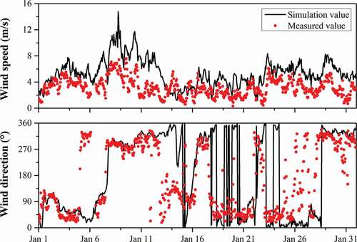
For the wind direction, the simulation effectively captures wind direction variations, with a R² value of 0.56. As shown in Table 4, the simulation is relatively good in January, with a MB of 5.83 °, and the RMSE of 36 °. The R² value for wind speed is 0.73. The simulation is relatively good in April, with MB of 1.03 m/s, and a RMSE of 2.29 m/s.

The comparative analysis between the measured and simulation results shows that the model can better reproduce the wind field and local meteorological processes in the simulation period, which provides a reliable meteorological background for the subsequent pollutant diffusion simulation.

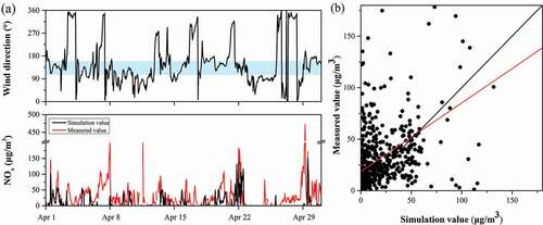
For the concentration evaluations, taking NO_x emissions from Enterprise A as example, demonstrates the relationship between the measured and simulation values at M2 station was downwind of the emission sources in 2019. When the wind direction is approximately 100°–140°, the M2 station is only affected by emissions from Enterprise A. The time series of the measured and simulation results are presented in Figure 4, and the correlation between the simulation and measured concentrations is provided.

Figure 4. Time series of (a) wind direction (the blue shadow represents the downwind direction of emission sources for M2 station (wind direction is about 100°~140°)), the measured and simulation results of the NOx concentrations (?g/m^3) and (b) the correlation between the simulation and measured concentrations at M2 station

It should be noted that, in this section, we used the actual emissions from Enterprise A as the emission inventory to carry out the CALPUFF simulation to verify the simulation effect of pollutant concentration. However, the introduction of the following sections is based on the simulation results of the baseline emission scenario described in Section 2.1, which used the current emission standard concentrations as the emission inventory.

The simulation captured the changes in the NO_x concentration, and the peak observed concentration was in good agreement with the simulated peak concentration when the M2 station was downwind of the emission sources (Figure 4(a)). During the simulation period, we selected the hours during which the M2 station was downwind of the emission sources to study the correlation between the simulation and measured concentrations (Figure 4(b)). The MB is −5.77 µg/m³ and the RMSE is 8.98 µg/m³, with a correlation coefficient of 0.67, indicating that the simulation results were generally credible compared with the measured values.

The simulation values of pollutant concentrations were usually lower than the measured values during several periods. One major reason is that the emission data used in the simulation in this section may underestimate the actual emission of Enterprise A. However, the error caused by this reason can be avoided in this study. As mentioned above, the emission concentrations used in the CALPUFF model to draw conclusions are the current emission standard concentrations instead of actual emissions. Another reason might be the neglect of other emission sources near the M2 station area (e.g., emissions from adjacent enterprises and biogenic emissions), which makes it difficult to quantitatively predict concentrations caused by uncertain and variable emissions (Kesarkar et al. 2007).

Results

Comprehensive analysis of pollutant ground level concentration under the baseline emission scenario

Compliance analysis of pollutant ground level concentration

For the conventional pollutants, the maximum ground level concentrations on annual average scale of SO₂, NO_x, PM₁₀, and PM_2.5 were 0.58 µg/m³, 6.41 µg/m³, 0.54 µg/m³, and 0.35 µg/m³, respectively. Compared with the zero-impact concentration limits (Table 3), under the baseline emission scenario, the emissions of SO₂, PM₁₀, and PM_2.5, meets the corresponding limits, while NO_x is out, and its maximum ground-level concentration exceeded the zero-impact concentration limit of 1.41 µg/m³.

In terms of spatial distribution, the annual average concentrations of conventional pollutants are similar (Figure 5), showing several high-value centers located in the northwest, west, southwest, and south of the chimneys, respectively. The ground-level concentrations of pollutants near the chimneys and in the northeast are lower than those recorded elsewhere. The annual maximum ground level concentration was in the northwest of the chimneys and at the boundary of the SCIP. The maximum concentrations of SO₂, NO_x, PM₁₀ and PM_2.5 were 1.48 ~ 2.18 km away from the chimneys.

Figure 5. Spatial distribution of annual average concentration of pollutants. The concentration is the average of the annual simulation results; the red contour line is the scope of the chemical industry park, and the black contour line covers the area that exceeds the zero-impact limits

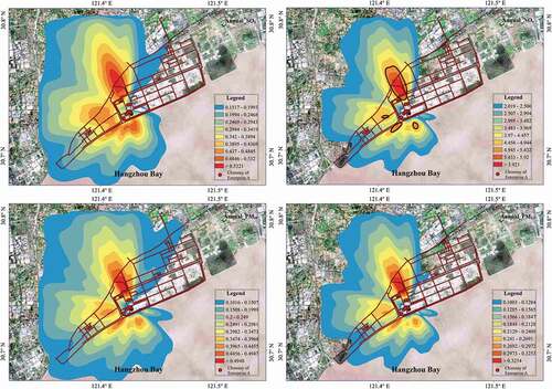
The annual average NO_x concentration is not up to the limit, and the areas that exceed the zero-impact concentration limits are distributed in the northwest, west, southwest, and southeast of the chimneys. The two exceed the limit areas in the south are small and located in Hangzhou Bay, and the largest exceed-limit area is in the northwest of the chimneys, which extends from the enterprise boundary, covering from the boundary to the periphery of the park.

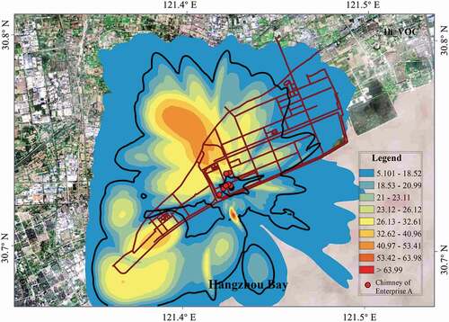
For the 1-hour average concentrations of the characteristic pollutant, VOCs (benzene) is 77.16 µg/m³, which is not up to the zero-impact concentration limit, and the concentration exceeds the zero-impact concentration limits by 68.16 µg/m³, with the 97.62% mean compliance rate.

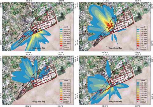
The spatial distributions of the 1-hour average concentrations of VOCs (benzene) are shown in Figure 6. The high-concentration centers are mainly distributed in the south, southwest and northwest of the chimneys. The maximum concentration is distributed in Hangzhou Bay, approximately 1.5 km from chimneys. The exceed-limit area of VOCs is large and extends to the southwest and north sides around the chimneys, covering most part of the SCIP and extending to its periphery. However, the ground-level concentration of VOCs is relatively low near the chimneys and achieves zero impact.

Figure 6. Spatial distribution of the 1-hour average concentration of volatile organic compounds (VOCs). The concentration is the maximum 1-hour ground level concentrations of VOCs (benzene) on each grid in the annual simulation results

Different characteristics of the wind field in different seasons also affect the pollutant concentration. The 1-hour average concentration distribution of VOCs (benzene) in each season is shown in Figure 7.

Figure 7. Spatial distribution of 1-hour average concentration of VOCs (benzene) during four seasons (shown in the order of winter, spring, summer, autumn; the concentration refers to the maximum 1-hour ground level concentrations of pollutants on each grid in the annual simulation results)

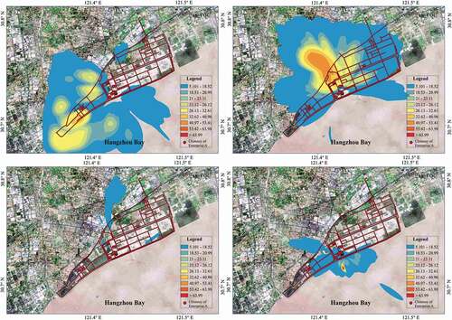
The 1-hour average concentrations of VOCs in the four seasons were the highest in the downwind direction of the high-frequency wind of all recorded VOCs. However, due to the shorter average time, the distribution of the 1-hour average concentration was more easily affected by special meteorological conditions. There is a significant difference between seasonal 1-hour average concentration distributions of VOCs, and all of them failed to meet the zero-impact concentration limits. The maximum concentrations are 35.83 µg/m³, 49.57 µg/m³, 12.03 µg/m³, and 77.16 µg/m³ in winter, spring, summer, and autumn, respectively. The ground level concentrations are lowest in summer and highest in autumn, and the exceed-limit areas of VOCs are largest in spring. Compared with those of other seasons, the average wind speed in spring in this area is the lowest (Figure 2), and the meteorological conditions are more stable than those in other seasons, which was not conducive to the diffusion of pollutants. Moreover, in autumn, due to the high frequency of special meteorological conditions, the maximum ground level concentration appears during this season. Under the meteorological conditions in spring and autumn, more stringent zero-impact emission limits are required.

Influence of short-term concentration of conventional pollutants

To conduct a more comprehensive study on zero-impact emissions of Enterprise A, the short-term concentration characteristics of 24-hour and 1-hour average time scales were also analyzed.

• (2) 24-hour average concentration

The maximum 24-hour average concentrations of SO₂, NO_x, PM₁₀, and PM_2.5 are 9.73 µg/m³, 137.74 µg/m³, 12.97 µg/m³ and 8.43 µg/m³, respectively. For 24-hour average concentrations, none of the four pollutants meet the corresponding 10% of the Level I standard (Table 3) under the baseline emission scenario, and the concentrations exceed the limit by 4.73 µg/m³, 127.74 µg/m³, 7.97 µg/m³, and 4.93 µg/m³, respectively.

In terms of spatial distribution, the 24-hour average concentrations of SO₂, NO_x, PM₁₀, and PM_2.5, show similar characteristics, and there are several high-concentration centers in all directions from the chimneys (Figure 8). Similar to the distribution of annual average concentration, the maximum 24-hour average concentrations of the four pollutants were all distributed northwest of the chimneys, approximately 0.65 ~ 1.46 km from the chimneys. However, the concentrations of pollutants northeast of the chimneys are low.

Figure 8. Spatial distribution of 24-hour average concentration of pollutants. The concentration refers to the maximum 24-hour average concentration of pollutants on each grid in the annual simulation results, and the black contour line covers the area that exceeds the 10% concentration

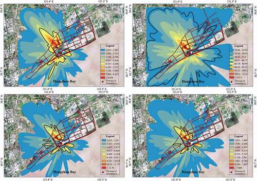
The area exceeding 10% of the Level I standard (i.e., exceedingly concentrated area) of NO_x was the most widely distributed, covering the whole SCIP and its surroundings, except for some areas parallel to the coastline located northeast of the chimneys. The extension range of the northwest mainland was larger than that of the Hangzhou Bay in the southeast. The exceedingly concentrated areas of SO₂, PM₁₀, and PM_2.5, were similar in spatial distribution, both in the northwest and southeast of the chimneys. However, the exceedingly concentrated areas of PM₁₀ and PM_2.5 were more scattered and distributed near the chimneys, while that of SO₂ was more concentrated, and the extension distances were further.

Using SO₂ as an example, the seasonal distribution of pollutant concentrations was analyzed. The 24-hour average concentration distributions of SO₂ in the four seasons are shown in Figure 9. The analysis of the other pollutants is presented in Appendix A.

Figure 9. Spatial distribution of 24-hour average concentration of SO2 during four seasons

As shown in Figure 9, there is a good correspondence between the spatial distributions of the 24-hour average concentration of SO₂ and the prevailing wind in each season. The SO₂ concentration exceeds 10% of the Level I standard during all seasons except summer. In winter, the maximum 24-hour average concentration is 7.34 µg/m³, exceeding 2.34 µg/m³, and it appears southwest of the chimneys, approximately 1.05 km away. In spring, the maximum concentration is 9.73 µg/m³, exceeding 4.73 µg/m³, and appears approximately 2.11 km away northwest of the chimneys. In autumn, the maximum concentration is 9.06 µg/m³, exceeding 4.06 µg/m³, and appears approximately 1.43 km away southwest of the chimneys. For seasonal distribution of 24-hour average concentrations, the SO₂ ground-level concentrations are lowest in summer but highest in spring, together with the largest exceed-concentration areas.

• (2) 1-hour average concentration

From the perspective of 1-hour average concentrations, the maximum 1-hour average concentrations of SO₂ and NO_x were 99.72 µg/m³ and 1679 µg/m³, respectively, exceeding the corresponding 10% of the Level I standard by 84.72 µg/m³ and 1654 µg/m³, respectively. The distance between the area with maximum concentration and chimney was approximately 1.5 ~ 1.63 km.

The spatial distributions of 1-hour average concentrations of SO₂ and NO_x are similar (Figure 10), and the high concentration areas are more intense than those of annual and 24-hour average concentrations, mainly distributed north and northwest of the chimneys. The maximum concentrations are distributed in Hangzhou Bay to the southeast of the chimneys.

Figure 10. Spatial distribution of 1-hour average concentration of pollutants

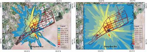
The farthest boundary of the NO_x concentration area was close to the boundary of the simulation area. That is, the exceed-concentration area covered most of the simulation area, and was beyond the scope of the simulation area in some directions. However, the ground level concentration of NO_x met the 10% of the Level I standard in a small area approximately 0.36 km away from the chimneys. As for SO₂, the exceed-concentration area was perpendicular to the coastline and extended to the southeast and northwest around the chimneys, covering part of the SCIP and extending to the outer area. The 1-hour concentration analysis of SO₂ and NO_x in each season is shown in Appendix A.

In general, for Enterprise A under the baseline emission scenario, NO_x and VOCs (benzene) failed to achieve zero-impact emissions. The maximum ground level concentration of NO_x exceeded the zero-impact concentration limit by 1.41 µg/m³, and VOCs (benzene) exceeded by 68.16 µg/m³. The common exceed-limit areas were northwest of the chimneys, covering the northern boundary of the SCIP and extending northward to the surroundings. There were also exceedingly limited areas distributed along the northeast-southwest direction of the park boundary southwest of the chimneys. In addition, there were common exceed-limit areas in Hangzhou Bay south of the chimneys.

For the short-term average concentration of conventional pollutants, their maximum ground-level concentrations exceed the corresponding 10% of the Level I standard (Table 2), and the distribution of the exceed-concentration area is wider than that of the exceed-limit area.

In addition to the emission scenario, the zero-impact emissions of Enterprise A were also affected by the meteorological conditions. The high-concentration areas were usually located downwind of the prevailing wind and at a certain distance from the chimneys, and the exceedingly limited areas were also usually located in these areas. In general, the wind conditions during spring in this region have put forward more stringent requirements for Enterprise A to achieve zero-impact emissions.

Determination of zero-impact concentration limits

Based on the simulation results of CALPUFF under the baseline emission scenario of Enterprise A, all situations of pollutants exceeding the zero-impact concentration limits in corresponding average times were selected, and the zero-impact emission limit of each pollutant was calculated according to the method introduced in Section 3.2.

According to the calculation results, the emission standards of some pollutants currently implemented in Enterprise A should be tightened to achieve zero-impact emissions under the baseline emission scenario. The zero-impact emission limits of all the pollutants are listed in Table 5.

Table 5. Zero-impact emission limits. (unit: mg/m³)

No.	Pollutant	Average time	Zero-impact emission limits (m$\mathbf{g}/m^3$)	The gap with current emission standards (m$\mathbf{g}/m^3$)	Tighten situation
1	SO2	Annual	50	0	balanced
2	NOx	Annual	78	−22	22% stricter
3	PM	Annual	10	0	balanced
4	VOCs (benzene)	1-hour	0.32	−3.68	92% stricter

The gap with current emission standards = zero-impact emission limits – current emission standards.

For the current emission standard of the typical petrochemical Enterprise A, the emissions of SO₂ and PM meet the zero-impact emission limits; however, the emission limits of NO_x and VOCs (benzene) need to be adjusted. The zero-impact emission limits of SO₂, NO_x, PM, and VOCs (benzene) determined in our study were 50 mg/m³, 78 mg/m³, 10 mg/m³ and 0.32 mg/m³, respectively. Compared with the current emission standard of Enterprise A, the emission limit of NO_x should be tightened by 22% (i.e., the emission concentration should be adjusted to 78 mg/m³) to work as zero-impact emission limit. For VOCs (benzene), the current emission standard should be tightened by 92% (i.e., adjusted to 0.32 mg/m³), and at the same time the fugitive emission should be reduced by the same proportion (i.e., controlled below 11.47 ton/a) to achieve zero-impact emissions.

After the adjustments, and compared with other industry emission standards, the zero-impact emission limits of PM are consistent with the ultra-low emission limits in China, while those of SO₂ and NO_x are slightly higher than the ultra-low emission limits. The zero-impact emission limit of VOCs (benzene) is 3.68 mg/m³ lower than the current emission standard of the SCIP, but only 0.68 mg/m³ lower than the local emission standard (regardless of industries) of Shanghai (DB31/933-2015).

Short-term concentration analysis of conventional pollutants based on the zero-impact emission limits

The zero-impact emission limits of conventional pollutants of Enterprise A obtained in this study are based on the long-term impact of conventional pollutants and are determined by the deduction made of the simulation results. The short-term concentration of conventional pollutants is not regarded as a constraint condition for determining the zero-impact emission limits. However, the short-term effects of pollutants on the environmental quality and human health are also crucial. Therefore, the short-term impact of conventional pollutants under the zero-impact emission scenario was further analyzed.

If Enterprise A adjusts the current emission standards according to the zero-impact emission limits obtained in this study, the comparison between the ground-level concentration of conventional pollutants in the short-term average time and their corresponding 10% of the Level I standards are shown in Figure 11.

Figure 11. Comparison of the short-term pollutant concentration with the corresponding 10% of the Level I standard in Enterprise A. The blue and green lines refer to 10% of the Level I standard of 24-hour and 1-h average concentration, respectively

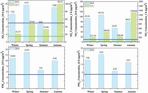
The maximum 24-hour and 1-hour average concentrations of SO₂ are 9.72 µg/m³ and 99.72 µg/m³, respectively, exceeding the corresponding 10% of the Level I standard. For the four seasons, all the 24-hour and 1-hour average concentrations will exceed the 10% concentrations, except for the 24-hour average concentration in summer. To make the 24-hour average concentration reach the corresponding 10% concentration, it is necessary to tighten the emission limit by 48% to 26 mg/m³. Moreover, tightening the emission limit by 84% to 8 mg/m³ will make the 1-hour average concentration reach the corresponding 10% concentration.

The maximum 24-hour and 1-hour average concentrations of NO_x are 107.43 µg/m³ and 1309.62 µg/m³, respectively. And the ground level concentrations are 30.3 µg/m³ and 369.38 µg/m³ lower than those under the baseline emission scenario, respectively. However, the concentrations for each season exceed the corresponding 10% of the Level I standard. To make the 24-hour average concentration reach the corresponding 10% concentration, the emission limit should be tightened by 91% to 9 mg/m³. As for the 1-hour average concentration, it is necessary to tighten the emission limit by 98% to 2 mg/m³ to reach the corresponding 10% concentration.

The maximum 24-hour average concentrations of PM₁₀ and PM_2.5 are 12.97 µg/m³ and 8.43 µg/m³, respectively, exceeding the corresponding 10% of the Level I standard, and the 24-hour average concentrations for the four seasons will exceed the corresponding 10% concentration. To make the 24-hour average concentration of PM reach the corresponding 10% concentration, the emission limit should be tightened by 60% to 4 mg/m³.

Overall, the zero-impact emission limits defined in this study were based on the concentration of the longest average time in Level I of the Chinese National Ambient Air Quality Standard. For conventional pollutants, achieving zero-impact emissions in the long-term average time is the first step for enterprises to further reduce emissions. However, for the shorter-term average time, there is still room for further tightening the zero-impact emission limits.

Discussion

For enterprises, there are various options to achieve zero-impact emissions in actual production activities, including the height and distribution of chimneys, as well as different technological processes. However, the adjustment suggestions for emission limits given in this study only focus on the actual height and distribution of the existing chimneys of Enterprise A. In actual production activities, in addition to adjusting the emission limits of each pollutant, enterprises can also reduce the ground-level concentration of pollutants by increasing the chimney height or adjusting the position of the chimney. Moreover, enterprises can adjust the emission concentration in different proportions based on the emission characteristics of each production process to achieve zero-impact emissions. Future research will be carried out in combination with the production process and emission height, to provide more diversified countermeasures to realize zero-impact emissions.

For different spatial scales, the realization of zero-impact emissions at the industrial park scale depends on its realization at the enterprise scale. In terms of the method of controlling pollutant emissions, concentration control is the first issue to be considered in the practice of enterprise emission reduction compared with total quantity control. Considering the controllability of point source emissions, our study focused on the emission concentration from each chimney of a typical enterprise to study the zero-impact emission limits, which is regarded as a breakthrough in zero-impact emission practices, which requires more urgent and operational research. However, the study of zero-impact emissions in a certain area will inevitably involve the problem of total quantity control and its optimization, which is a different pollution control technology from this study (Varga and Kuehr 2007).

For zero-impact emissions in a larger area, the emission impact of the entire area is not a simple accumulation of the emission impact of each sub-area. In terms of the zero-impact emission at the park or city scale with more emission chimneys and larger study areas, the zero-impact emission limits will be different from the results in this study.

Conclusion

Based on previous related research on zero emissions, the concept of zero-impact emissions was proposed in this study, and the zero-impact concentration limits at the enterprise level were determined with reference to the Level I standard of the Chinese National Ambient Air Quality Standard. Taking a typical petrochemical enterprise in SCIP as an example, and based on the technical route of concentration control, the determination method of zero-impact emission limits of air pollutants in the enterprise was studied using the CALPUFF model. The main conclusions are as follows:

When the concentration of a pollutant reaches the zero-impact concentration limit at a certain control area after dilution and diffusion, meaning the emission will not have any adverse impact on the environmental quality or health effects in this area, such emissions are defined as zero-impact emissions. In this study, 10% of the Level I standard of each pollutant in the Chinese National Ambient Air Quality Standard on the annual average time scale were determined as the zero-impact concentration limits for conventional pollutants, and 9 µg/m³ in the 1-hour average time scale was determined for VOCs (benzene) according to the Best Management Practices for Monitoring and Reducing Emissions of Volatile Organic Compounds by the U.S. EPA. When the maximum ground-level concentration of pollutants does not exceed the zero-impact concentration limit, the emission concentration is determined as the zero-impact emission limit.

Under the baseline emission scenario of Enterprise A, NO_x and VOCs (benzene) failed to achieve zero-impact emissions in the corresponding average time. The annual average concentration of NO_x exceeded the zero-impact concentration limit by 28.2% (1.41 µg/m³), and the 1-hour average concentration of VOCs (benzene) exceeded the zero-impact concentration limit by 757.33% (68.16 µg/m³).

In terms of spatial distribution, the exceedingly limited areas of zero impact in Enterprise A were located northwest of the chimneys, and southwest of the chimneys in Hangzhou Bay. According to the simulation results for the four seasons, the wind conditions in spring were more unfavorable for the enterprise to achieve zero-impact emissions.

For the current emission standards of Enterprise A, SO₂ and PM can achieve zero-impact emissions, while the emissions of NO_x and VOCs (benzene) fail to do so. Based on the simulation, the zero-impact emission limits of SO₂, NO_x, PM, and VOCs (benzene) of Enterprise A are 50 mg/m³, 78 mg/m³, 10 mg/m³ and 0.32 mg/m³, respectively. Therefore, the current emission standards for NO_x and VOCs (benzene) need to be tightened by 22% and 92%, respectively. At the same time, the fugitive emission of benzene should be controlled below 11.47 ton/a to achieve zero-impact emissions.

After the implementation of zero-impact emission limits, the annual, 24-hour, and 1-hour average concentration of NO_x will be reduced by 1.41 µg/m³, 30.3 µg/m³, and 369.38 µg/m³. The 1-hour average VOCs (benzene) concentration will be decreased by 68.2 µg/m³.

Industrial parks are general enterprise communities that are distributed worldwide. In China, there are 2543 national and provincial industrial parks (National Development and Reform Commission et al., 2018). Through a case study, this paper solves the environmental management issue, which is of universal significance for chemical industry parks. The concept of zero-impact emissions and the determination method of zero-impact concentration limits proposed in our study can be used as references for related research on cutting emissions. Although the conclusion of this study on the emission limits is not suitable for direct application to other enterprises, the calculation method of the zero-impact emission limit can be used without modification. Furthermore, the zero-impact emission limits on the park scale can be determined after a comprehensive evaluation based on the calculation results of multiple enterprises.

Acknowledgments

This research was supported by the Science and Technology Commission of Shanghai Municipality, China (18DZ1206704).

Disclosure statement

No potential conflict of interest was reported by the author(s).

Supplementary material

Supplemental data for this paper can be accessed on the publisher’s website

Additional information

Funding

This work was supported by the the Science and Technology Commission of Shanghai Municipality, China [18DZ1206704].

Notes on contributors

Li He

Li He is a doctoral candidate of the Department of Environmental Science and Engineering at Fudan University, China. Her research is mainly engaged in numerical simulation of atmospheric pollution.

Huiyu Jin

Huiyu Jing is a doctoral candidate of the Department of Environmental Science and Engineering at Fudan University, China. Her research is mainly engaged in environmental mathematical model.

Jiajia Wang

Jiajia Wang is a master graduate student of the Department of Environmental Science and Engineering at Fudan University, China. She majored in environmental big data.

Jian Li

Jian Li is a master graduate student of the Department of Environmental Science and Engineering at Fudan University, China. He works in the Junyue Energy and Technology (Shanghai) Co, Ltd, Shanghai, China.

Qi Yu

Qi Yu is an associate professor of the Department of Environmental Science and Engineering at Fudan University, China. She majored in the simulation and prediction of atmospheric environmental pollutants.

Weichun Ma

Weichun Ma is a professor of the Department of Environmental Science and Engineering at Fudan University, China. His research interests include environmental mathematical model and geographic information system.

References

- Akyuz, E., and B. Kaynak. 2019. Use of dispersion model and satellite SO2 Retrievals for environmental impact assessment of coal-fired power plants. Sci. Total Environ 689: 808–19. Elsevier B.V. doi:https://doi.org/10.1016/j.scitotenv.2019.06.464.
- Bai, S. B., Y. Q. Wen, L. He, Y. M. Liu, Y. Zhang, Q. Yu, and W. C. Ma. 2020. Single-vessel plume dispersion simulation: Method and a case study using CALPUFF in the Yantian Port Area, Shenzhen (China). Int. J. Environ. Res. Public Health 17 (21):1–28. doi:https://doi.org/10.3390/ijerph17217831.
- Bezyk, Y., D. Oshurok, M. Dorodnikov, and I. Sówka. 2021. Evaluation of the CALPUFF model performance for the estimation of the urban ecosystem CO2 flux. Atmos. Pollut. Res 12 (3):260–77. doi:https://doi.org/10.1016/j.apr.2020.12.013.
- Biswas, K., A. Chatterjee, and J. Chakraborty. 2020. Comparison of air pollutants between Kolkata and Siliguri, India, and its relationship to temperature change. J. Geovisualization Spat. Anal 4 (2020):25. doi:https://doi.org/10.1007/s41651-020-00065-4.
- Brown, M. A., B. Beasley, F. Atalay, K. M. Cobb, P. Dwiveldi, J. Hubbs, D. M. Iwaniek, S. Mani, D. Matisoff, J. E. Mohan, et al. 2021. Translating a global emission-reduction framework for subnational climate action: A case study from the State of Georgia. Environ. Manage 67 (2):205–27. Springer US. doi:https://doi.org/10.1007/s00267-020-01406-1.
- Cao, J., R. Garbaccio, and M. S. Ho. 2009. China’s 11th five-year plan and the environment: Reducing SO2 emissions. Rev. Environ. Econ. Policy 3 (2):231–50. doi:https://doi.org/10.1093/reep/rep006.
- Cui, Y. Z., L. Wang, L. Jiang, M. Y. Liu, J. H. Wang, K. F. Shi, and X. J. Duan. 2021. Dynamic spatial analysis of NO2 pollution over China: Satellite observations and spatial convergence models. Atmos. Pollut. Res 12 (3):89–99. Elsevier B.V. doi:https://doi.org/10.1016/j.apr.2021.02.003.
- Dresser, A. L., and R. D. Huizer. 2011. CALPUFF and AERMOD model validation study in the near field: Martins Creek revisited. J. Air Waste Manag. Assoc 61 (6):647–59. doi:https://doi.org/10.3155/1047-3289.61.6.647.
- Ehrlich, C., G. Noll, W. Kalkoff, G. Baumbach, and A. Dreiseidler. 2007. PM10,PM2.5 and PM1.0—Emissions from industrial plants—Results from measurement programmes in Germany. Atmos. Environ 41:6236–54. doi:https://doi.org/10.1016/j.atmosenv.2007.03.059.
- Elbir, T., N. Mangir, M. Kara, S. Simsir, T. Eren, and S. Ozdemir. 2010. Development of a GIS-based decision support system for urban air quality management in the city of Istanbul. Atmos. Environ 44 (4):441–54. Elsevier Ltd. doi:https://doi.org/10.1016/j.atmosenv.2009.11.008.
- Fan, H., C. F. Zhao, and Y. K. Yang. 2020. A comprehensive analysis of the spatio-temporal variation of urban air pollution in China during 2014–2018. Atmos. Environ. 220 (April 2019):117066. Elsevier Ltd. doi:https://doi.org/10.1016/j.atmosenv.2019.117066.
- Filonchyk, M., and H. W. Yan. 2018. The characteristics of air pollutants during different seasons in the urban area of Lanzhou, Northwest China. Environ. Earth Sci 77:22. doi:https://doi.org/10.1007/s12665-018-7925-1.
- Giaiotti, D., D. Oshurok, and O. Skrynyk. 2018. The chernobyl nuclear accident 137Cs cumulative depositions simulated by means of the CALMET/CALPUFF modelling system. Atmos. Pollut. Res 9 (3):502–12. Elsevier B.V. doi:https://doi.org/10.1016/j.apr.2017.11.007.
- Guo, D. P., R. Wang, and P. Zhao. 2020. Spatial distribution and source contributions of PM2.5 concentrations in Jincheng, China. Atmos. Pollut. Res 11 (8):1281–89. Elsevier B.V. doi:https://doi.org/10.1016/j.apr.2020.05.004.
- He, L., J. J. Wang, Y. M. Liu, Y. Zhang, C. He, Q. Yu, and W. C. Ma. 2021. Selection of onshore sites based on monitoring possibility evaluation of exhausts from individual ships for Yantian Port, China. Atmos. Environ 247 (August 2020):118187. doi:https://doi.org/10.1016/j.atmosenv.2021.118187.
- Huang, Y. Y., Q. W. Yan, and C. R. Zhang. 2018. Spatial-temporal distribution characteristics of PM 2.5 in China in 2016. J. Geovisualization Spat. Anal. 2:12.
- Indumati, S., R. B. Oza, Y. S. Mayya, V. D. Puranik, and H. S. Kushwaha. 2009. Dispersion of pollutants over land-water-land interface: Study using CALPUFF model. Atmos. Environ. 43 (2):473–78. Elsevier Ltd. doi:https://doi.org/10.1016/j.atmosenv.2008.09.030.
- Jia, H. H., J. T. Huo, Q. Y. Fu, Y. Sen Duan, Y. F. Lin, X. D. Jin, X. Hu, and J. P. Cheng. 2020. Insights into chemical composition, abatement mechanisms and regional transport of atmospheric pollutants in the Yangtze river delta region, China during the COVID-19 outbreak control period. Environ. Pollut. 267: 115612. Elsevier Ltd. doi:https://doi.org/10.1016/j.envpol.2020.115612.
- Jiao, X. M., X. Liu, Y. Z. Gu, X. Bin, X. Wu, S. M. Wang, and Y. Zhou. 2020. Satellite verification of ultra-low emission reduction effect of coal-fired power plants. Atmos. Pollut. Res. 11 (7):1179–86. doi:https://doi.org/10.1016/j.apr.2020.04.005.
- Kaufman, N., A. R. Barron, W. Krawczyk, P. Marsters, and H. McJeon. 2020. A near-term to net zero alternative to the social cost of carbon for setting carbon prices. Nat. Clim. Chang. 10 (11):1010–14. Springer US. doi:https://doi.org/10.1038/s41558-020-0880-3.
- Kesarkar, A. P., M. Dalvi, A. Kaginalkar, and A. Ojha. 2007. Coupling of the weather research and forecasting model with AERMOD for pollutant dispersion modeling. A case study for PM10 dispersion over Pune, India. Atmos. Environ. 41:1976–88. doi:https://doi.org/10.1016/j.atmosenv.2006.10.042.
- Krajnc, D., M. Mele, and P. Glavič. 2007. Improving the economic and environmental performances of the beet sugar industry in Slovenia: Increasing fuel efficiency and using by-products for ethanol. J. Clean. Prod. 15 (13–14):1240–52. doi:https://doi.org/10.1016/j.jclepro.2006.07.037.
- Kuehr, R. 2000 Strategic sustainable development: A comparison of current approaches (executive summary of a UNU/ZEF workshop in Carnoules/ France June 2000). Tokyo/Berlin.
- Kuehr, R., 2007. Towards a sustainable society: United Nations University’s Zero Emissions Approach. J. Clean. Prod. 15:1198–1204 https://doi.org/https://doi.org/10.1016/j.jclepro.2006.07.020.
- Lee, B. K., and S. W. Cho. 2003. Strategies for emission reduction of air pollutants produced from a chemical plant. Environ. Manage. 31 (1):42–49. doi:https://doi.org/10.1007/s00267-002-2789-1.
- Levy, I. 2013. A national day with near zero emissions and its effect on primary and secondary pollutants. Atmos. Environ. 77: 202–12. Elsevier Ltd. doi:https://doi.org/10.1016/j.atmosenv.2013.05.005.
- Li, J. X., Z. X. Wang, L. L. Chen, L. L. Lian, Y. Li, L. Y. Zhao, S. Zhou, Mao, X. X., Huang, T., Gao, H., and Ma, J. M. 2020. WRF-chem simulations of ozone pollution and control strategy in petrochemical industrialized and heavily polluted Lanzhou City, Northwestern China. Sci. Total Environ. 737:139835. Elsevier B.V. doi:https://doi.org/10.1016/j.scitotenv.2020.139835.
- Li, K., D. J. Jacob, H. Liao, J. Zhu, V. Shah, L. Shen, K. H. Bates, Q. Zhang, and S. X. Zhai. 2019b. A two-pollutant strategy for improving ozone and particulate air quality in China. Nat. Geosci. 12 (11):906–10. doi:https://doi.org/10.1038/s41561-019-0464-x.
- Li, K., D. J. Jacob, H. Liao, L. Shen, Q. Zhang, and K. H. Bates. 2019a. Anthropogenic drivers of 2013–2017 trends in summer surface ozone in China. Proc. Natl. Acad. Sci. U. S. A. 116 (2):422–27. doi:https://doi.org/10.1073/pnas.1812168116.
- Liang, T., S. S. Wang, C. Y. Lu, N. Jiang, W. Q. Long, M. Zhang, and R. Q. Zhang. 2020. Environmental impact evaluation of an iron and steel plant in China: Normalized data and direct/indirect contribution. J. Clean. Prod. 264: 121697. Elsevier Ltd. doi:https://doi.org/10.1016/j.jclepro.2020.121697.
- Lin, Y. C., C. Y. Lai, and C. P. Chu. 2021. Air pollution diffusion simulation and seasonal spatial risk analysis for industrial areas. Environ. Res. 194 (6):110693. Elsevier Inc. doi:https://doi.org/10.1016/j.envres.2020.110693.
- Liu, Y. P., J. G. Wu, D. Y. Yu, and R. F. Hao. 2018. Understanding the patterns and drivers of air pollution on multiple time scales: The case of Northern China. Environ. Manage 61 (6):1048–61. Springer US. doi:https://doi.org/10.1007/s00267-018-1026-5.
- MacIntosh, D. L., J. H. Stewart, T. A. Myatt, J. E. Sabato, G. C. Flowers, K. W. Brown, D. J. Hlinka, and D. A. Sullivan. 2010. Use of CALPUFF for exposure assessment in a near-field, complex terrain setting. Atmos. Environ. 44 (2):262–70. Elsevier Ltd. doi:https://doi.org/10.1016/j.atmosenv.2009.09.023.
- Matsuno, Y., N. Itsubo, H. Hondo, and K. Nakano. 2013. LCA in Japan in the twenty-first century. Int. J. Life Cycle Assess. 18 (1):278–84. doi:https://doi.org/10.1007/s11367-012-0473-0.
- Matthews, H. D., and K. Caldeira. 2008. Stabilizing climate requires near-zero emissions. Geophys. Res. Lett. 35 (4). doi: https://doi.org/10.1029/2007GL032388.
- McNider, R. T., and A. Pour-Biazar. 2020. Meteorological modeling relevant to mesoscale and regional air quality applications: A review. J. Air Waste Manag. Assoc. 70 (1):2–43. Taylor & Francis. doi:https://doi.org/10.1080/10962247.2019.1694602.
- National Development and Reform Commission, Ministry of Science and Technology of China, Ministry of Natural Resources of China, Ministry of Housing and Urban-Rural Development of China, Ministry of Commerce of China and General Adminstration of Costoms of China. 2018. Review announcement of industrial park in China (2018) [Chinese]. Beijing: National Development and Reform Commission, Ministry of Science and Technology of China, Ministry of Natural Resources of China, Ministry of Housing and Urban-Rural Development of China, Ministry of Commerce of China and General Adminstration of Costoms of China.
- Ozkurt, N., D. Sari, N. Akalin, and B. Hilmioglu. 2013. Evaluation of the impact of SO2 and NO2 emissions on the ambient air-quality in the çan-bayramiç region of Northwest Turkey during 2007-2008. Sci. Total Environ 456–457 (2):254–66. Elsevier B.V. doi:https://doi.org/10.1016/j.scitotenv.2013.03.096.
- Scire, J. S., D. G. Strimaitis, and R. J. Yamartino. 2000a. A user’s guide for the CALPUFF dispersion model (Version 5). Concord, MA: Earth Tech, Inc. http://www.src.com/calpuff/download/CALPUFF_UsersGuide.pdf
- Scire, J. S., D. G. Strimaitis, and R. J. Yamartino. 2000b. A user’s guide for the CALMET meteorological model (Version 5). Concord, MA: Earth Tech, Inc. http://www.src.com/calpuff/download/CALMET_UsersGuide.pdf.
- Skamarock, W. C., J. B. Klemp, J. Dudhia, D. O. Gill, D. M. Barker, M. G. Duda, X.-Y. Huang, W. Wang, and J. G. Powers, 2008 A description of the advanced research WRF version 3. NCAR Tech. Note NCAR/TN-475+STR, 113. doi:https://doi.org/10.5065/D68S4MVH
- Sproul, E., J. Barlow, and J. C. Quinn. 2020. Time-resolved cost analysis of natural gas power plant conversion to bioenergy with carbon capture and storage to support net-zero emissions. Environ. Sci. Technol. 54 (23):15338–46. doi:https://doi.org/10.1021/acs.est.0c04041.
- Suzuki, M. 2000. Constructing material circulation process toward a zero emissions society. Report of the Scientific-Grant-in-Aid of the Ministry of Education, No. 292. Tokyo: Research Institute of Industrial Engineering, University of Tokyo (Japanese)
- Tang, H. Y., P. Jiang, J. He, and W. C. Ma. 2020. Synergies of cutting air pollutants and CO2 emissions by the end-of-pipe treatment facilities in a typical Chinese integrated steel plant. Sustain 12 (12):1–23. doi:https://doi.org/10.3390/su12125157.
- Tang, L., J. B. Qu, Z. F. Mi, X. Bo, X. Y. Chang, L. D. Anadon, S. Y. Wang, X. Xue, S. Li, X. Wang, et al. 2019. Substantial emission reductions from Chinese power plants after the introduction of ultra-low emissions standards. Nat. Energy 4 (11):929–38. Springer US. doi:https://doi.org/10.1038/s41560-019-0468-1.
- Tian, D. Y., J. H. Fan, H. B. Jin, H. C. Mao, D. Geng, S. G. Hou, P. Zhang, and Y. F. Zhang. 2020. Characteristic and spatiotemporal variation of air pollution in Northern China based on correlation analysis and clustering analysis of five air pollutants. J. Geophys. Res. Atmos. 125 (8):1–12. doi:https://doi.org/10.1029/2019JD031931.
- U.S. Environmental Protection Agency (U.S. EPA). 2015. Petroleum refinery sector risk and technology review and new source performance standards. EPA/HQ/OAR/2010/0682. U.S. EPA, Washington, DC. https://www.govinfo.gov/content/pkg/FR-2015-12-01/pdf/2015-26486.pdf .
- United Nations Environment Programme (UNEP). 1997. Environmental management of industrial estates, 150. Industry and Environment. UNEP.
- Varga, M., and R. Kuehr. 2007. Integrative approaches towards zero emissions regional planning: Synergies of concepts. J. Clean. Prod. 15 (13–14):1373–81. doi:https://doi.org/10.1016/j.jclepro.2006.07.009.
- Wang, J. J., X. M. Lu, Y. T. Yan, L. G. Zhou, and W. C. Ma. 2020. Spatiotemporal characteristics of PM2.5 concentration in the Yangtze river delta urban agglomeration, China on the application of big data and wavelet analysis. Sci. Total Environ 724: 138134. Elsevier B.V. doi:https://doi.org/10.1016/j.scitotenv.2020.138134.
- Wang, S. M., X. H. Yu, Y. Z. Gu, J. Yuan, Y. Zhang, Y. B. Chen, and F. H. Chai. 2018. Discussion of emission limits of air pollutants for‘near-zero emission’coal-fired power plants. Res. Of Environ. Sci. 31 (6):975–84. (Chinese).
- Wang, S. W., Q. Zhang, R. V. Martin, S. Philip, F. Liu, M. Li, X. Jiang, and K. He. 2015. Satellite measurements oversee China’s sulfur dioxide emission reductions from coal-fired power plants. Environ. Res. Lett. 10 (11):114015. IOP Publishing. doi:https://doi.org/10.1088/1748-9326/10/11/114015.
- Willmott, C. J. 1981. On the validation of models. Phys. Geogr. 2 (2):184–94. doi:https://doi.org/10.1080/02723646.1981.10642213.
- Wu, H., Y. Zhang, Q. Yu, and W. C. Ma. 2018. Application of an integrated Weather Research and Forecasting (WRF)/CALPUFF modeling tool for source apportionment of atmospheric pollutants for air quality management: A case study in the urban area of Benxi, China. J. Air Waste Manag. Assoc. 68 (4):347–68. doi:https://doi.org/10.1080/10962247.2017.1391009.
- Xia, C., B. Ye, J. Jiang, and Y. Shu. 2020. Prospect of near-zero-emission IGCC power plants to decarbonize coal-fired power generation in China: Implications from the GreenGen project. J. Clean. Prod. 271: 122615. Elsevier Ltd. doi:https://doi.org/10.1016/j.jclepro.2020.122615.
- Yang, B., Y. M. Wei, Y. B. Hou, H. Li, and P. T. Wang. 2019. Life cycle environmental impact assessment of fuel mix-based biomass co-firing plants with CO2 capture and storage. Appl. Energy 252 (June):113483. Elsevier. doi:https://doi.org/10.1016/j.apenergy.2019.113483.
- Yang, H. Z., J. Liu, K. Jiang, J. Meng, D. Guan, Y. Xu, and S. Tao. 2018. Multi-objective analysis of the co-mitigation of CO2 and PM2.5 pollution by China’s iron and steel industry. J. Clean. Prod. 185: 331–41. Elsevier Ltd. doi:https://doi.org/10.1016/j.jclepro.2018.02.092.
- Yantovski, E., J. Gorski, B. Smyth, and J. Ten Elshof. 2004. Zero-emission fuel-fired power plants with ion transport membrane. Energy 29 ( 12-15 SPEC. ISS.):2077–88. doi:https://doi.org/10.1016/j.energy.2004.03.013.
- Yim, S. H. L., J. C. H. Fung, and A. K. H. Lau. 2010. Use of high-resolution MM5/CALMET/CALPUFF system: SO2 apportionment to air quality in Hong Kong. Atmos. Environ. 44 (38):4850–58. Elsevier Ltd. doi:https://doi.org/10.1016/j.atmosenv.2010.08.037.
- Zhang, C. Z., D. J. Liu, S. Y. Zou, and S. Liu. 2020. Implementation status of ultra-low emission in China’s iron and steel industry. Environ. Impact. Assess. 42 (4):1–5. (Chinese).
- Zhang, W. J., H. Q. Li, B. Chen, Q. Li, X. J. Hou, and H. Zhang. 2015. CO2 emission and mitigation potential estimations of China’s primary aluminum industry. J. Clean. Prod. 103: 863–72. Elsevier Ltd. doi:https://doi.org/10.1016/j.jclepro.2014.07.066.
- Zhao, D. Y., Y. N. Jin, and S. Q. Zhang. 2016. Cost-effectiveness analysis of pollution emission reductionmeasures and ultra-low emission policies for coal-fired power plants. J. Environ. Sci. (China). 36 (9):2841–48. (Chinese).
- Zheng, B., D. Tong, M. Li, F. Liu, C. P. Hong, G. N. Geng, H. Y. Li, Li, X., Peng, L. Q., Qi, J. Yan, L., Zhang, Y. X., Zhao, H. Y., Zheng, Y. X., He, K. B., and Zhang, Q. 2018. Trends in China’s anthropogenic emissions since 2010 as the consequence of clean air actions. Atmos. Chem. Phys. 18 (19):14095–111. doi:https://doi.org/10.5194/acp-18-14095-2018.
- Zheng, H., S. F. Kong, Y. Y. Yan, N. Chen, L. Q. Yao, X. Liu, F. Q. Wu, Y. Cheng, Z. Niu, S. Zheng, et al. 2020. Compositions, sources and health risks of ambient Volatile Organic Compounds (VOCs) at a petrochemical industrial park along the Yangtze river. Sci. Total Environ. 703:135505. Elsevier B.V. doi:https://doi.org/10.1016/j.scitotenv.2019.135505.
- Zhou, H. G., L. Zhao., C. S. Chen, and M. Li. 2015. Research on the technical route and industrial application of near-zero emission of coal-fired power plants supplied with shenhua coal. Electric Power 48 (5):89–96. (Chinese).