A novel assessment framework for improving air quality monitoring network layout

ABSTRACT

Redundant stations in the air quality monitoring network (AQMN), not only cause high maintenance and operation costs, but also affect the performance of air quality assessment. This study presents a novel framework for identifying the redundant stations and selecting the corresponding alternatives in AQMN. The framework composes three main steps. Firstly, we identify the redundant stations by correlation analysis and stepwise regression methods. Secondly, we determine the corresponding alternative stations by cluster analysis and correspondence analysis methods. Finally, the final optimization results are verified by the support vector regression. We perform empirical evaluations of the framework using Shanghai’s AQMN. The results show that Xuhui, Zhangjiang, Shiwuchang, and Pudong New Area are four redundant pollution monitoring stations. Alternatives for each type of pollutant for these redundant stations are proposed and the adjusted layout of AQMN is verified with historical data. The framework proposed in this study can effectively improve the layout of AQMN, which could be applied to other cities or regions to improve the integrity of pollution information and reduce the monitoring costs.

Implications: In this study, we set up a comprehensive framework. A case study proves that the framework we proposed can help countries identify redundant stations, so as to reduce the monitoring costs, improve the monitoring efficiency, and provide technical support for governments to implement accurate air quality control measures.Four particularly important aspects were highlighted in this work: (i) A new framework was constructed that combined regression and prediction for the first time to analyze and validate pollutant data; (ii) The framework used Stepwise Regression to improve previous methods for identifying redundant monitoring stations, effectively improving identification efficiency; (iii) The framework used Support Vector Regression to make predictions to verify the final results of the optimized layout, which was ignored in previous studies. (iv) This framework can be applied to any city or region, which has important practical significance for improving the comprehensiveness and accuracy of pollution monitoring in various cities.

Introduction

Air pollution is a globally recognized environmental issue that poses a major hazard to human health. The World Health Organization reports that approximately 4.2 million people die each year from outdoor air pollution (http://www.who.int/airpollution/en/). Air pollution, such as haze caused mainly by fine particulate matter (PM_2.5), gains increasing public concern (Kim et al. 2018; Xing et al. 2016; Zhu et al. 2019). Air quality monitoring network (AQMN) is the key infrastructure for assessing urban air quality. It provides air quality information based on which authorities take measures to improve air quality. The European Union began air quality monitoring earlier than most nations, and it has established a comprehensive monitoring network and applied advanced monitoring techniques (http://www.empt.int/). The U.S. Environmental Protection Agency began to establish and operate State and Local Air Monitoring Stations and National Air Monitoring Stations in 1970s, which monitor ambient air quality for indicator pollutants and evaluate air quality for its compliance with the National Ambient Air Quality Standard. So far, they have established relatively well-developed AQMNs (https://www.epa.gov/). AQMN construction in China began in the mid-1970s and continued until the mid-to-late 1980s. In the early 1990s, the AQMN entered an adjustment and optimization period. Since 2000, monitoring projects have been changed from SO₂, NOx, and total suspended particulates to SO₂, NOx, PM₁₀. By 2020, China had set up more than 5000 monitoring stations at the national, provincial, municipal, and county levels, and the air quality monitoring network had been set up to release real-time monitoring data and the calculated air quality index for six indicators: PM₁₀, PM_2.5, SO₂, NO₂, O₃, and CO. The data from this network is available to the public. Hourly data can be reliably used to monitor air pollution with reasonable accuracy. Many scholars used these data for research. Zhang et al. (2017) used a 10-year data set of daily PM₁₀ concentrations from four stations in Taiyuan, China, to predict a short-term series of PM₁₀ concentrations. Luo et al. (2021) analyzed the spatial and temporal distribution characteristics of PM_2.5 pollution and the relationships between PM_2.5 concentration and meteorological factors based on the monitoring data and meteorological data in Harbin in 2017.

AQMN can assist authorities in developing monitoring strategies (Mofarrah and Husain 2010). The key to AQMN layout is the reasonable distribution of monitoring stations and the determination of a reliable number of sampling points for air quality measurement. The air quality network management should focus on monitoring the largest possible targeted area, maximizing coverage of spatial gradient information of air pollutants, and reducing fixed stations within the AQMN to a reliable, non-redundant digital (Galán-Madruga 2021).

However, there are still many issues with the existing city-based AQMNs, among which the potentially inefficient layout of monitoring stations is the major one. The layout of AQMN, designed many years ago, may not fit the current layout of the city. With the economic and social development, the adjustment of industrial structure, and population flow, the original layout of monitoring stations cannot adapt to the current needs. The government may add some new monitoring stations according to the urban development, and therefore, some original monitoring stations may become redundant due to adjustment of layout and other reasons. Many studies have already proved the existence of redundant monitoring stations in the AQMNs. For example, Lu, He, and Dong (2011) used a combination of principal-components analysis and cluster analysis to classify the sources of SO₂, NO_2, and PM₁₀ in Hong Kong. It was found that there were redundant stations in the AQMN in Hong Kong. Zhao et al. (2015) used the principal component analysis and assignment methods to analyze the layout of the Shanghai air quality monitoring network, and found that the layout of air quality monitoring stations in Shanghai was unsatisfying. Wang et al. (2018) combined cluster analysis and correspondence analysis to comprehensively identify redundant stations in Xi’an city in China, and found alternative stations for the redundant stations. The existence of redundant monitoring stations will lead to high monitoring costs and reduce monitoring efficiency. Although these studies used various methods to identify redundant stations and their replacement stations, there were still some problems in the methods adopted, which may cause the identification of redundant stations to be inaccurate. Moreover, there was no verification of the final results of the improved layout, which made it difficult to judge the effectiveness of the result. To solve these problems, this study established a new framework, which can identify redundant monitoring stations more accurately than previous methods. At the same time, the final results of the improved layout were verified to ensure the scientific nature of the framework.

Literature review

Most monitoring stations are located in densely populated urban areas. However, clustered stations may present similar air pollution information and similar trends. And they are often redundant for pollution assessment, especially on the regional or national scale. In recent years, many scholars have been studying AQMN, analyzing the existence of redundant monitoring stations. Pope and Wu (2014) considered that a regional monitoring network should effectively reflect spatial pollution patterns and trends and provide all population groups with sufficient information on quality of the air. Macpherson et al. (2017) proposed a national model for optimizing multi-pollutant emission control strategies based on the mixed integer programming model. The model combined detailed air quality and emissions control information and helped states explore collaborative strategies for air quality management. The study demonstrated that one way to optimize the monitoring network was to identify redundant stations that should be excluded because they encumbered the monitoring process and introduced interpretation biases on air quality. Li et al. (2019) believed that instead of maintaining redundant stations, it was more cost effective to place the stations in the areas that can improve the representation of AQMN. Under the constraints on available resources, it was thus suggested to remove some redundant monitoring stations in order to reallocate resources and establish stations in other areas of monitoring interests.

Many research focused on the methods for identifying redundant stations. For example, Lu, He, and Dong (2011) used a combination of principal-components analysis and cluster analysis to classify the sources of SO₂, NO₂, and PM₁₀ in Hong Kong and to evaluate the performance of Hong Kong’s AQMN. It was found that there were redundant stations in the AQMN in Hong Kong. Hwang and Chan (2012) described a statistical method for assessing site redundancy of urban air monitoring networks in reporting daily Pollutant Standard Index (PSI), average concentrations, and the number of exceedances. This statistical method identified significant redundancy in monitoring stations for one-year measurements of two air monitoring networks in Taiwan: five redundant stations were identified out of fifteen monitoring stations in the Taipei area and eight redundant stations out of eighteen monitoring stations in the Kaohsiung area. Using this method, we can not only determine the number of redundant stations to be downsized, but also the priority of station removal. Zhao et al. (2015) used the principal component analysis and assignment methods to analyze the layout of the Shanghai AQMN, and found redundant monitoring stations. Their analysis also suggested that, in addition to industrial, transportation, construction, and population influences inside Shanghai, external pollutants significantly affected Shanghai’s air quality. Hao and Xie (2018) considered that AQMNs played an important role in identifying the spatiotemporal patterns of air pollution, and they needed to be deployed effectively with a minimum number of stations. Therefore, they designed an optimal monitoring network based on Weather Research and Forecaster-California PUFF (WRF-CalPuff) model and genetic algorithm (GA). The maximization of coverage with minimum overlap and the ability to detect violations of standards were the design objectives for redistributed networks. Wang et al. (2018) combined cluster analysis and correspondence analysis to identify redundant stations in Xi’an, China and also identified the alternative stations for the replacement. Castro and Pires (2019) applied principal component analysis to analyze the spatial distribution of NO₂, O₃ and PM₁₀ concentration profiles in Porto, Portugal. The analysis performed concluded that it was necessary to reduce the monitoring points of NO₂ and O₃ and optimize the current number of PM₁₀ monitoring stations. Stolz, Huertas, and Mendoza (2020) suggested using a clustering integration approach to identify similar and redundant stations by combining three clustering techniques: principal component analysis, hierarchical clustering, and k-means. The results showed that the clustering integration method was a reliable tool to identify similar stations. Su et al. (2020) proposed a method for predicting O₃ concentrations based on a kernel extremal learning machine combined with SVR, and preprocessed the data using wavelet transforms and partial least-squares regression to verify the validity of the method. The study used precursor observations, meteorological observations, and hourly O₃ concentration observations for the summer from 2014 to 2016 in China’s Nanjing Industrial Zone. They found that the combination of the kernel extremal learning machine with SVR improved predictions of O₃ concentrations. It had important application value for improving urban air quality, making control strategy and optimizing urban air quality monitoring network. Malinovic-Milicevic et al. (2021) described generation and performances of feedforward neural network models for predicting daily maximum 1-hour ozone concentration and 8-hour average ozone concentration at a traffic and a background station in the urban area of Novi Sad, Serbia. Models showed a good performance in forecasting days with the high values over a certain threshold. Research was helpful for managers to predict pollutant concentration effectively for subsequent management. Galán-Madruga (2021) proposed methodology sets criteria for identifying non-redundant stations in the air quality monitoring network and also allowed for proper evaluation of the representation of fixed monitoring sites in the air quality monitoring network.

Unfortunately, few of the studies described above provided a complete framework for identifying redundant stations. Although the study of Wang et al. (2018) provided a framework, the method for identifying redundant monitoring stations is not optimal. Principal component analysis (PCA) and assignment method (AM) were used to identify redundant monitoring stations. PCA may retain components that contribute little to independent variables in order to achieve cumulative contribution rate. As a result, in the study of redundant stations, monitoring stations with low contribution will be retained as main components for subsequent analysis, which will lead to inaccurate selecting of redundant stations. The AM was suitable for small square arrays, and once the data is large, the arrangement will be complicated, slow and error-prone in calculation. Therefore, the applicability of the method had concerns in the case of a large number of monitoring stations and complex data arrangement. Moreover, none of these studies evaluated the effectiveness of AQMN after deleting the redundant monitoring stations, leaving the effectiveness of the proposed AQMN unknown. Therefore, there is a need to provide a new framework to improve the layout of AQMN with new methods and add steps for evaluation of the result.

This study presents a novel framework for identifying the redundant stations and selecting the corresponding alternatives in AQMN to maximize the efficiency of the monitoring stations. The innovation of the present study is as follows: (i) This study uses stepwise regression (SWR) to identify redundant monitoring stations, with which method to retain or remove stations by gradually adding and validating each node to find replacements for the redundant monitoring stations. The logic of this method is that a variable is removed from the regression equation when it is introduced into the regression equation and tested as insignificant. In this way, the method ensures that the regression equation contains only significant variables. This method does not introduce monitoring stations with very low contribution rate to achieve the cumulative contribution rate like PCA. Also, it effectively avoids the complex arrangement requirements of the assignment method for huge data, and it can establish the optimal regression equation between one monitoring station and other monitoring stations. In other words, SWR can effectively replace PCA and AM. (ii) Support vector regression (SVR) is used to test the final results of the improved layout to ensure that the new proposed framework accurately monitor all six types of pollutants. Aim of the study is to improve the layout of the urban air quality monitoring stations to reduce their costs and improve monitoring efficiency.

Materials and methods

As shown in Figure 1, we build a framework for optimizing the layout of AQMN, including three main steps: (i) identify the redundant stations using Correlation Analysis (COA) and Stepwise Regression (SWR); (ii) determine alternative stations for redundant stations using Cluster Analysis (CA) and Corresponding Analysis (CSA); (iii) verify our results using Support Vector Regression (SVR).

Figure 1. Framework for optimizing the layout of AQMN.

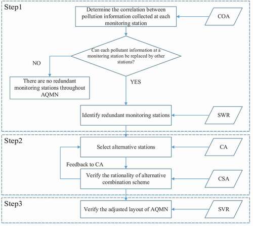
Step 1 Identify redundant stations

1) Determine the correlation between monitoring stations using COA

We used COA to determine whether there were potentially redundant monitoring stations in the AQMN. First, we calculated the correlations in the monitoring network for each pollutant. For that pollutant, a weak correlation (r < 0.5) for data at two monitoring stations indicates that neither station can replace the other station (i.e., there is no redundancy)(Liu et al. 2018; Sahu and Patra 2021; Wang et al. 2018); conversely, a strong correlation (r> 0.5) indicates that for that pollutant, one station could potentially replace another (i.e., there is redundancy). If data for all six pollutants at a given station can be provided by the other stations, then that station is potentially redundant.

2) Identify redundant stations using SWR

The basic idea of SWR is to introduce variables into the model one by one. After each explanatory variable is introduced, the F value is calculated to determine whether the model is statistically significant and a t test is carried out on newly introduced explanatory variables to determine whether they significantly improve the regression result. When the original explanatory variable becomes no longer significant due to the introduction of the new explanatory variable, it will be deleted from the model. If it remains significant, then both variables are retained in the regression equation. When this iterative process is finished, only significant variables are included in the regression equation. The iteration continues until no new variables are added and no old variables are deleted. We use forward selection for identifying redundant stations, as follows:

Step 1: For each station X_j, we develop a one-dimensional regression model with another station X_i. Then the F-test is performed, and if it passes the significance test, X_i is retained, otherwise X_i is removed.

(1) $Xj=\beta 0+\beta iXi+\epsilon {,}^{\hspace{0.17em}}i=1,\dots ,p\hspace{0.17em}j=1,\dots ,p(j\ne i)$(1)

Where $\beta i$ represents the regression coefficient, $\beta 0$ represents the constant term and $\epsilon$ represents the random error.

Step 2: Arrange X_i in descending order according to $\beta i$, then introduce X_i one by one, observe the F-test of the regression equation after the introduction of X_i. Retain X_i if all the tests pass, otherwise remove X_i. Until p-1 monitoring stations are introduced into the regression equation for testing. We obtain a linear combination of a monitoring station X_j with the other monitoring stations X_i that pass the test.

Step 3: Calculate the strength of the fitting (R²) of the above X_j linear combination equation. If R² > 0.7 (Chen et al. 2013; Shi, Lau, and Ng 2017; Vlachokostas et al. 2011), then we assume that X_j can be replaced by a linear combination of X_i. If R² < 0.7, it cannot be replaced.

For one station, repeat the above steps for the six pollutants respectively to obtain the R² of the six fitting equations. If five of the six R² are greater than 0.7, the station is considered to be redundant and can be replaced.

Step 2 Determine alternative stations

1) Select alternative stations using CA

Yidana, Ophori, and Banoeng-Yakubo (2008) proposed hierarchical clustering analysis, so we used hierarchical clustering analysis to select alternative stations. If no alternative stations could be found, then this station is not a real redundant station. Therefore, this step could also be regarded as a verification of the redundant station identified in Step 1.

Hierarchical clustering is one of the most commonly used methods in CA, and it is an efficient method to perform the clustering for large databases. We used rescaled distance clustering combinations (RDCC) to measure the distance between stations. The two variables with the smallest RDCC distance are combined into a new cluster.

The steps in the hierarchical clustering approach are as follows.

Step 1: Classify each monitoring station into its own class, so that a total of N classes are obtained, and so that each class contains only one monitoring station. The distances between pairs of classes are the distances between the monitoring stations.

Step 2: Based on the RDCC distance for the monitoring stations, the two stations with the smallest RDCC distance are grouped into one category, and the other stations remain in their original category. This step reduces the total number of classes by 1.

Step 3: Recalculate the distances between the new class and all the other classes.

Step 4: Repeat steps 2 and 3 until all of the monitoring stations have been grouped into one class (This class contains all N stations).

The analyses were performed using version 24 of IBM’s SPSS software.

2) Verify the rationality of alternative combination using CSA

CSA, which is also known as R-Q factor analysis, is a newly developed statistical analysis technique for multiple dependent variables that reveals the association between variables by analyzing interaction matrices consisting of qualitative variables. This method not only quantifies the results of CA but also helps to confirm whether one or more alternatives are feasible. The basic steps of CSA are as follows:

Step 1: Using the raw AQMN data, one-column tables of qualitative variables (monitoring stations and pollutants) are obtained. The Q-factor analysis table shows the contribution of each monitoring station to each pollutant.

Step 2: As long as the contribution of one or more alternative stations is equal to or greater than the contribution of a potentially redundant monitoring station, the alternative station or combination of stations can be used to replace the redundant monitoring station. This provides a quantitative confirmation that an alternative station or combination of alternative stations is a reasonable alternative to the redundant station.

Step 3 Verify the effectiveness of the proposed layout of AQMN using SVR

SVR is a way to apply support vector machines to regression problems. Its core idea is to find a separation hyperplane (i.e., a hypersurface) that minimizes the expected risk of producing an incorrect solution. We use historical data from monitoring stations and SVR to test the effectiveness of the adjusted AQMN layout.

For a certain pollutant, the alternative station of monitoring station X_j is monitoring station X_i. The historical data of X_j and X_i will be used to verify the result. The data is divided into training set and testing set. Using the data of the training set, an SVR model will be trained based on the input value of X_j and output value of X_i. Linear kernel function is used to train the SVR model. Based on the SVR model, X_i of monitoring station can be calculated using X_j in the test set, and then can be compared with real data of X_i in the test set. Finally, this study uses R² to verify the accuracy of the model.

(2) $R{\hspace{0.17em}}^2=\frac{(\sum _{i=1}^N(y{p}_{{ }^i}-\bar{y}p)(y{0}_{{ }^i}-\bar{y}0){)}^2}{\sum _{i=1}^N{(y{p}_{{ }^i}-\bar{y}p)}^2\sum _{i=1}^N{(y{0}_{{ }^i}-\bar{y}o)}^2}$(2)

Where y_pi and y_0i represent the predicted and true values of the monitoring data at time i, respectively, $\bar{y}p$ means the average value of the monitoring data for a pollutant obtained by prediction, and $\bar{y}0$ means the average value of the true data monitored by the monitoring station for the pollutant. N is the total sample size of monitoring stations.

The higher the R² value for a pollutant at a monitoring station, the better the prediction. In other words, the more effective the proposed layout of AQMN is because the regression model’s predictions can accurately represent it.

The analyses were performed using version 3.7 of Python software.

Results and discussion

Case study

Shanghai has a land area of 6340.5 km². It is located on the western coast of the Pacific Ocean, on the eastern edge of the Asian continent. Because many of the city’s heavy industries are located upwind of the city, much of the pollution from these industries is carried into Shanghai.

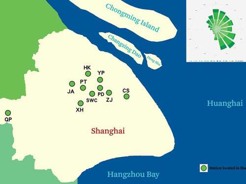
The current AQMN in Shanghai consists of 10 state-controlled monitoring stations: Jing’an (JA), Putuo (PT), Shiwuchang (SWC), Xuhui (XH), Hongkou (HK), Yangpu (YP), Pudong New Area (PD), Zhangjiang (ZJ), Chuansha (CS), and Qingpu (QP). Most of the stations are located in densely populated urban centers and a few are located in suburban residential areas with a low traffic flow. The characteristics of the 10 stations are shown in Table 1 and their locations are shown in Figure 2. These stations monitor the concentrations of PM_2.5, PM₁₀, SO₂, O₃, NO₂, and CO. The 1-hour or 24-hour average mass concentrations of these pollutants are available online, and we collected these data from the monitoring agency’s website (http://www.pm25china.net). The data we used were the 24-hour average mass concentrations of these six pollutants for the time period from 00:00 on 1 January 2014 to 23:59 on 31 December 2018.

Table 1. Characteristics of the 10 air quality monitoring stations

Station	Abbreviation	District	Monitoring environment
Jing’an	JA	Jing’an	Residential area
Putuo	PT	Putuo	Residential area
Shiwuchang	SWC	Huangpu	Residential area
Xuhui	XH	Xuhui	Residential area
Hongkou	HK	Hongkou	Residential area
Pudong New area	PD	Pudong	Residential area
Zhangjiang	ZJ	Pudong	Industrial High-Tech Park
Chuansha	CS	Pudong	Commercial area, high traffic
Qingpu	QP	Qingpu	Rural (background)
Yangpu	YP	Yangpu	Residential area

Figure 2. Locations of the 10 air quality monitoring stations in Shanghai city.

Identify redundant stations in Shanghai

1) Determine the correlation between monitoring stations using COA

We used COA to determine whether any of the monitoring stations in Shanghai’s AQMN were potentially redundant. Table 2 shows the correlations between monitoring stations for PM_2.5. Data for the other five pollutants are presented as supplemental Table A.1 to A.5. The correlations of O₃ and PM_2.5 are stronger than other pollutants because O₃ and PM_2.5 are secondary pollutants, and their reaction rates tend to smooth out the concentration field. Other pollutants, such as CO, SO₂, are primary pollutants that are directly emitted into the atmosphere by the source and less affected by the surrounding air than secondary pollutants that would interact with the surrounding pollutants.

Table 2. Analysis of the correlation (Pearson’s r) between monitoring stations for PM2.5

Stations	HK	JA	CS	PD	ZJ	PT	QP	SWC	XH	YP
HK	1
JA	0.667**	1
CS	0.697**	0.647**	1
PD	0.697**	0.799**	0.722**	1
ZJ	0.685**	0.797**	0.724**	0.972**	1
PT	0.682**	0.683**	0.698**	0.845**	0.829**	1
QP	0.569**	0.593**	0.622**	0.658**	0.658**	0.625**	1
SWC	0.691**	0.750**	0.726**	0.912**	0.903**	0.855**	0.643**	1
XH	0.697**	0.802**	0.711**	0.961**	0.951**	0.843**	0.655**	0.914**	1
YP	0.604**	0.703**	0.580**	0.754**	0.748**	0.675**	0.493**	0.799**	0.748**	1

Notes. **significant at p < 0.01 (two-tailed test).

In Table 2, r represents the correlation coefficient. In most cases, r > 0.5, and all correlations are statistically significant. For PM_2.5 and O₃, r > 0.7 in most cases, which indicates that there is a strong correlation between concentrations of these pollutants at the monitoring stations. For SO₂, the r for PT and QP is between 0.4 and 0.5. For CO, r for QP, YP, and the other stations is less than 0.5, showing a weak correlation. Therefore, this indicates that these monitoring stations are not easily replaced by other monitoring stations. Therefore, they are not redundant monitoring stations. The COA showed that in most cases, the 10 monitoring stations were strongly correlated, indicating that the AQMN contains potentially redundant stations. Therefore, we need to first identify the potentially redundant stations and then confirm that they are indeed redundant.

2) Identify redundant stations using SWR

We performed SWR analysis for the six pollutants based on data from the 10 monitoring stations. We will discuss the results for O₃ at HK as an example; analysis for the other stations and pollutants followed the same approach. As shown in Table 3, the CS had the greatest contribution to HK, and was introduced first into the regression equation. In this study, the criteria for retaining variables were P < .05 and collinearity < 10 based on the variance inflation factor (VIF); CS met both criteria. Next, PD met the criteria for inclusion, with VIF = 2.396. In the third step, PT was introduced. In the fourth step, YP was introduced. In the fifth step, JA was introduced. In the sixth step, ZJ was introduced, but the P value for PD increased to 0.693 (i.e., not significant) and the VIF increased to 11.015. As a result, PD was eliminated from the model. In the seventh step, the stations selected before this step were tested to determine whether they should be retained after elimination of the PD, and the requirements were met; as a result, they were retained. In the 8th step, the SWC was introduced. Thereafter, no other stations were introduced and none were eliminated, so the analysis was complete.

Table 3. SWR analysis of O₃ in Hongkou (HK). VIF, variance inflation factor

Model		Unstandardized coefficient			t statistic	P	Collinearity statistic
		β0	βi	Standard error			VIF
1	(constant)	8.079		1.212	6.667	< 0.001
	CS		0.805	0.015	53.819	< 0.001	1
2	(constant)	−0.03		1.149	−0.026	0.979
	CS		0.468	0.021	22.566	< 0.001	2.396
	PD		0.425	0.02	21.352	< 0.001	2.396
3	(constant)	−3.223		1.161	−2.777	0.006
	CS		0.387	0.022	17.889	< 0.001	2.762
	PD		0.333	0.021	15.542	< 0.001	2.922
	PT		0.222	0.022	10.2	< 0.001	2.563
4	(constant)	−5.543		1.186	−4.675	< 0.001
	CS		0.375	0.021	17.547	< 0.001	2.777
	PD		0.213	0.027	8.013	< 0.001	4.636
	PT		0.226	0.021	10.525	< 0.001	2.564
	YP		0.158	0.021	7.416	< 0.001	2.898
5	(constant)	−6.66		1.186	−5.614	< 0.001
	CS		0.349	0.022	16.198	< 0.001	2.882
	PD		0.149	0.028	5.288	< 0.001	5.318
	PT		0.198	0.022	9.112	< 0.001	2.676
	YP		0.15	0.021	7.109	< 0.001	2.908
	JA		0.145	0.023	6.348	< 0.001	3.102
6	(constant)	−5.947		1.183	−5.028	< 0.001
	CS		0.331	0.022	15.332	< 0.001	2.945
	PD		−0.016	0.04	−0.395	0.693	11.015
	PT		0.21	0.022	9.713	< 0.001	2.703
	YP		0.142	0.021	6.778	< 0.001	2.921
	JA		0.132	0.023	5.826	< 0.001	3.13
	ZJ		0.197	0.035	5.703	< 0.001	8.241
7	(constant)	−5.958		1.182	−5.039	< 0.001
	CS		0.331	0.022	15.341	< 0.001	2.933
	PT		0.208	0.021	9.916	< 0.001	2.544
	YP		0.139	0.02	7.046	< 0.001	2.601
	JA		0.131	0.022	5.851	< 0.001	3.03
	ZJ		0.187	0.024	7.8	< 0.001	3.979
8	(constant)	−6.209		1.183	−5.248	< 0.001
	CS		0.319	0.022	14.534	< 0.001	3.045
	PT		0.202	0.021	9.589	< 0.001	2.57
	YP		0.117	0.021	5.529	< 0.001	2.996
	JA		0.124	0.022	5.553	< 0.001	3.06
	ZJ		0.148	0.028	5.353	< 0.001	5.279
	SWC		0.094	0.032	2.887	0.004	5.838

Notes. The dependent variable:HK

Table 4 summarizes the R² from the SWR for one representative station JA, and identify the monitoring stations that contributed significantly to each pollutant based on the SWR analysis. Data for the other nine stations are presented as supplemental Table B.1 to B.9. The R² for all pollutants at QP was less than 0.6, whereas JA, HK, CS, and YP had only one pollutant with an R² greater than 0.7. PT had two pollutants with R² greater than 0.7, and XH, SWC, ZJ, and PD each had five to six pollutants with R² greater than 0.7, suggesting that pollutant concentrations at the latter four stations can be predicted well based on data from the other stations. Therefore, our preliminary results suggest that XH, SWC, PD, and ZJ stations are potentially redundant stations. The remaining six stations can potentially replace these four stations.

Table 4. Stepwise regression (SWR) results for JA Station

	R^2	Contributing stations
PM2.5	0.699	XH	YP	ZJ	HK	PD	QP	CS	PT	SWC
O3	0.693	PD	HK	PT	QP	ZJ	CS
PM10	0.622	ZJ	YP	CS	HK	SWC	QP
SO2	0.621	XH	YP	HK	CS	QP	ZJ
NO2	0.731	XH	PD	YP	HK	CS	PT	ZJ
CO	0.495	QP	YP	HK	XH	ZJ	PD

Notes. Boldfaced values represent R² > 0.7

Determine alternative stations in Shanghai

In a monitoring network, all the six pollutants monitored by each potential redundant station must be replaced by alternative stations. In this case, the potential redundant station was a truly redundant station. Otherwise, information will be lost. Therefore, we used CA to determine alternative stations for four potentially redundant stations and validated the redundant stations with CSA.

1) Select the alternative stations for XH, SWC, ZJ, and PD

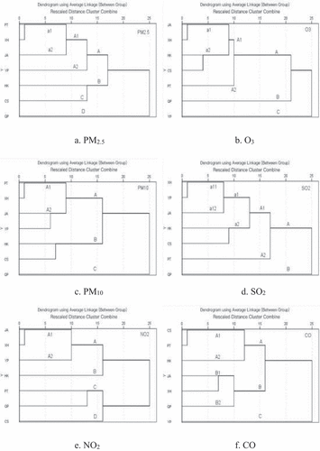
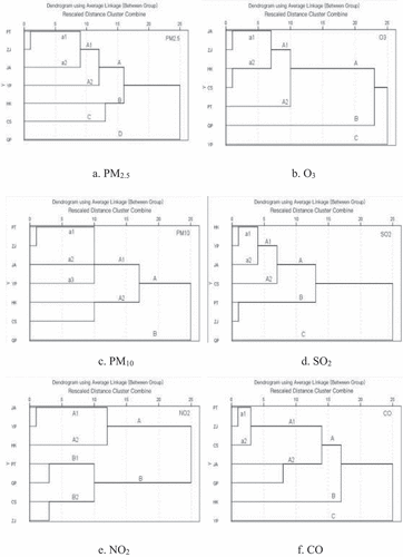
For XH, based on the RDCC distance, Figure 3 shows the CA dendrograms that determine the alternatives.

Figure 3. The dendrograms for the 7 monitoring stations in Shanghai after excluding SWC, ZJ, and PD.

(a) For PM_2.5, the a1 cluster includes XH and PT, suggesting that these clusters are monitoring similar PM_2.5 characteristics. Thus, PT can replace XH (Figure 3a).

(b) For O₃, JA can replace XH in the a1 cluster (Figure 3b).

(c) For PM₁₀, PT can replace XH in the A1 cluster (Figure 3c).

(d) For SO₂, YP can replace XH in the a11 cluster (Figure 3d).

(e) For NO₂, JA can replace XH in the A1 cluster (Figure 3e).

(f) For CO, JA can replace XH in the B1 cluster (Figure 3f).

For SWC, based on the RDCC distance, Figure 4 shows the CA dendrograms that determine the alternatives.

Figure 4. The dendrograms for the 7 monitoring stations in Shanghai after excluding XH, ZJ, and PD.

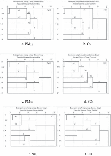
(a) For PM_2.5, PT can replace SWC in the a1 cluster (Figure 4a).

(b) For O₃, YP can replace SWC in the A cluster (Figure 4b).

(c) For PM₁₀, PT can replace SWC in the a1 cluster (Figure 4c).

(d) For SO₂, YP can replace SWC in the a11 cluster (Figure 4d).

(e) For NO₂, JA can replaced SWC in the A1 cluster (Figure 4e).

(f) For CO, QP, JA, HK, PT, or CS stations in cluster A can be used as alternative stations for SWC (Figure 4f).

For ZJ, based on the RDCC distance, Figure 5 shows the CA dendrograms that determine the alternatives.

Figure 5. The dendrograms for the 7 monitoring stations in Shanghai after excluding SWC, XH, and PD.

(a) For PM_2.5, PT can replace ZJ in the a1 cluster (Figure 5a).

(b) For O₃, JA can replace ZJ in the a1 cluster (Figure 5b).

(c) For PM₁₀, PT can replace ZJ in the a1 cluster (Figure 5c).

(d) For SO₂, ZJ can be replaced by PT in the B cluster (Figure 5d).

(e) For NO₂, CS can replace ZJ in the B2 cluster (Figure 5e).

(f) For CO, PT can replace ZJ in the a1 cluster (Figure 5f).

For PD, based on the RDCC distance, Figure 6 shows the CA dendrograms that determine the alternatives.

Figure 6. The dendrograms for the 7 monitoring stations in Shanghai after excluding SWC, XH, and ZJ.

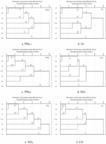
(a) For PM_2.5, PT can replace PD in the a1 cluster (Figure 6a).

(b) For O₃, YP can replace PD in the A1 cluster (Figure 6b).

(c) For PM₁₀, JA can replace PD in the a11 cluster (Figure 6c).

(d) For SO₂, YP can replace PD in the a1 cluster (Figure 6d).

(e) For NO₂, JA can replace PD in the a11 cluster (Figure 6e).

(f) For CO, CS can replace PD in the a1 cluster (Figure 6f).

To sum up, alternative monitoring stations can be found for the six pollutants for all four stations in the current AQMN, which ensure that XH, SWC, ZJ and PD are redundant stations in Shanghai’s AQMN. Some pollutants have multiple alternative monitoring stations, making the optimal choice of redundant monitoring stations unclear. For CO (Figure 4f), combinations of two or more of the QP, JA, HK, PT and CS stations can replace SWC. In the SWR, it was proved that YP contributed to CO of SWC. However, the CA showed that the information of the CO of YP was not similar to that of SWC, and therefore YP was not suitable as an alternative station to SWC. These results make it difficult to identify redundant monitoring stations that have more alternatives. To solve this problem, we used the Q-factor loading matrix approach, which is described in the next section.

2) Verify the rationality of alternative combination using CSA

We performed further analysis by creating a Q-factor load matrix (Table 5) to confirm our identification of redundant monitoring stations. Table 5 shows the contribution of each monitoring station to the monitoring of each pollutant. If the contribution of the alternative pollutant monitoring stations determined in the CA results is equal to or greater than that of the redundant monitoring stations, this indicates that the appropriate alternative stations have been selected. For example, the contribution of the alternative station PT (0.113) is greater than that of PD (0.105) for PM_2.5, which indicates that it is reasonable to replace PD with PT. For CO, no one station has a contribution greater than SWC (0.110), but for any combination of QP, JA, HK, PT, and CS stations, such as HK (0.098) and PT (0.107), their combined contribution is 0.205 (0.098 + 0.107), which is greater than that of SWC (0.110). This proves that the combination of HK and PT can be used as an alternative to SWC. Therefore, any combination of two or more of these stations can replace SWC. This analysis confirms that the alternative stations we chose are reasonable. Overall, the Q-factor load matrix approach confirms our accuracy in identifying redundant monitoring stations.

Table 5. Q-factor loading matrix

Q-factor loading matrix.
Stations	Marginal values for each pollutant
	PM2.5	O3	PM10	SO2	NO2	CO
HK	0.104	0.103	0.090	0.104	0.096	0.098
JA	0.097	0.112	0.104	0.096	0.106	0.101
CS	0.096	0.091	0.108	0.111	0.107	0.097
PD	0.105	0.101	0.102	0.102	0.106	0.098
ZJ	0.103	0.102	0.104	0.108	0.103	0.105
PT	0.113	0.093	0.109	0.101	0.102	0.107
QP	0.067	0.080	0.086	0.073	0.083	0.077
SWC	0.109	0.103	0.104	0.100	0.093	0.110
XH	0.108	0.105	0.101	0.102	0.105	0.103
YP	0.097	0.109	0.091	0.102	0.098	0.103
Sum of marginal values	1.000	1.000	1.000	1.000	1.000	1.000

Notes. Boldfaced values represent the contributions of the four potentially redundant stations for monitoring each pollutant.

In summary, Table 6 presents the adjusted layout of AQMN, where the four redundant stations PD, ZJ, SWC and XH can be replaced by their alternatives. For different types of pollutants, different alternatives are selected. For example, for PM_2.5, PD can be replaced by PT. While for O₃, PD can be replaced by YP. For CO for SWC, no one station can replace this station, but any combination of QP, JA, HK, PT, and CS stations can be a replacement for it.

Table 6. The possible alternatives for the four redundant monitoring stations

Pollutants	PD Alternatives	ZJ Alternatives	SWC Alternatives	XH Alternatives
PM2.5	PT	PT	PT	PT
O3	YP	JA	YP	JA
PM10	JA	PT	PT	PT
SO2	YP	PT	YP	YP
NO2	JA	CS	JA	JA
CO	CS	PT	QP+JA+HK+PT+CS	JA

Verify the adjusted layout of AQMN using SVR

To further verify our result, we tested the predictive ability of the adjusted layout of AQMN using SVR. We utilized historical pollutants data of each station from 2014 to 2018. 3/4 of the data was used for training and the rest of 1/4 of the data was used for validation. Specifically, we used the data from 2014 to 2017 as training data and the 2018 data for validation. Table 7 shows the predictive ability of the alternatives. According to SVR, the coefficient of determination in the PM_2.5 concentration models are greater than 0.80, indicating that the fitting effect is very good; the coefficients of determination in the PM₁₀, O₃, SO₂ and NO₂ concentration models are all greater than 0.60, indicating that the fitting effect is good; the coefficients of determination in the CO concentration models are all greater than 0.50, indicating that the fitting effect is acceptable (Gryech et al. 2020; Liu et al. 2021; Zaman et al. 2021).

Table 7. Predictive ability (R²) for the redundant monitoring stations in Shanghai

Redundant stations	R^2
	PM2.5	O3	PM10	SO2	NO2	CO
XH	0.85	0.66	0.60	0.63	0.66	0.54
SWC	0.85	0.67	0.81	0.68	0.60	0.59
ZJ	0.80	0.65	0.77	0.61	0.63	0.55
PD	0.84	0.66	0.61	0.60	0.63	0.58

Conclusion

This study aimed to improve the efficiency of AQMN by identifying redundant monitoring stations and selecting alternative stations. We developed a framework that combined three steps to accurately identify redundant monitoring stations, propose alternative stations and verify the result. A case study of AQMN in Shanghai has been performed using this framework. First, we used COA analysis to calculate correlations among the monitoring stations and reveal the existence of potentially redundant stations, followed by identification of the potentially redundant stations (XH, SWC, ZJ, PD) using SWR. Then the alternative schemes of redundant stations were found through CA and the alternative combination schemes were tested by CSA. Finally, we verified that the proposed new AQMN layout was effective using SVR. Our framework not only selected alternatives for each of the four redundant monitoring stations but also verified their accuracy.

Compared with the original AQMN, the improved AQMN can effectively reduce the cost and ensure the accuracy of monitoring information. Our results therefore had important practical significance for improving the efficiency of urban pollution monitoring network. Based on the framework used in this study, the adjusted layout of the air quality monitoring network saved money, which can be invested in monitoring or research on other environmental pollutants. The conclusions of our study can help the authorities to manage it better in two ways. On the one hand, from the perspective of cost optimization, after identifying redundant stations, the monitoring cost can be effectively reduced by replacing redundant stations with information from the alternative stations. On the other hand, from an information integrity perspective, identifying redundant stations facilitates information management. If a station goes into a downtime operational condition, the missing information can be recovered from the alternative stations, which helps the authorities to better manage the information. The framework proposed in this study can be effectively applied to other cities or regions to reduce monitoring costs and improve environmental benefits.

Disclosure statement

No potential conflict of interest was reported by the author(s).

Data availability statement

The data that support the findings of this study are available from the corresponding author upon reasonable request.

Supplementary material

Supplemental data for this paper can be accessed on the publisher’s website.

Additional information

Funding

This work was supported by grants from the National Social Science Foundation of China [Projects No. 18AZD005] and the National Natural Science Foundation of China [Project No. 71874108].

Notes on contributors

Laijun Zhao

Laijun Zhao is distinguished professor, doctoral supervisor and dean of School of Management, University of Shanghai for Science and Technology. He has been studying some important issues in emergent environmental governance for a long time.

Yi Zhou

Yi Zhou is a postgraduate student at University of Shanghai for Science and Technology.

Ying Qian

Ying Qian is a professor at university of Shanghai for Science and Technology.

Pingle Yang

Pingle Yang is a postdoctoral fellow at the University of Shanghai for Science and Technology.

Lixin Zhou

Lixin Zhou is a postdoctoral fellow at the University of Shanghai for Science and Technology.

References

- Castro, M., and J. C. M. Pires. 2019. Decision support tool to improve the spatial distribution of air quality monitoring sites. Atmos. Pollut. Res. 10 (3):827–34. doi:https://doi.org/10.1016/j.apr.2018.12.011.
- Chen, Y., R. Shi, S. Shu, and W. Gao. 2013. Ensemble and enhanced PM10 concentration forecast model based on stepwise regression and wavelet analysis. Atmos. Environ. 74:346–59. doi:https://doi.org/10.1016/j.atmosenv.2013.04.002.
- Galán-Madruga, D. 2021. A methodological framework for improving air quality monitoring network layout. Applications to environment management. J. Environ. Sci. 102:138–47. doi:https://doi.org/10.1016/j.jes.2020.09.009.
- Gryech, I., M. Ghogho, H. Elhammouti, N. Sbihi, and A. Kobbane. 2020. Machine learning for air quality prediction using meteorological and traffic related features. J. Ambient. Intell. Smart Environ. 12 (5):379–91. doi:https://doi.org/10.3233/AIS-200572.
- Hao, Y., and S. Xie. 2018. Optimal redistribution of an urban air quality monitoring network using atmospheric dispersion model and genetic algorithm. Atmos. Environ. 177:222–33. doi:https://doi.org/10.1016/j.atmosenv.2018.01.011.
- Hwang, J.-S., and -C.-C. Chan. 2012. Redundant measurements of urban air monitoring networks in air quality reporting. J. Air Waste Manage. Assoc. 47 (5):614–19. doi:https://doi.org/10.1080/10473289.1997.10463682.
- Kim, D., Z. Chen, L. F. Zhou, and S. X. Huang. 2018. Air pollutants and early origins of respiratory diseases. Chronic Dis. Transl. Med. 4 (2):75–94. doi:https://doi.org/10.1016/j.cdtm.2018.03.003.
- Li, J., H. Zhang, Y. Luo, X. Deng, M. L. Grieneisen, F. Yang, B. Di, and Y. Zhan. 2019. Stepwise genetic algorithm for adaptive management: Application to air quality monitoring network optimization. Atmos. Environ. 215:116894. doi:https://doi.org/10.1016/j.atmosenv.2019.116894.
- Liu, B., Q. Zhao, Y. Jin, et al. 2021. Application of combined model of stepwise regression analysis and artificial neural network in data calibration of miniature air quality detector. Sci. Rep. 11:3247. doi:https://doi.org/10.1038/s41598-021-82871-4:3247.
- Liu, Y., J. Wu, D. Yu, and R. Hao. 2018. Understanding the patterns and drivers of air pollution on multiple time scales: The case of Northern China. Environ. Manage. 61 (6):1048–61. doi:https://doi.org/10.1007/s00267-018-1026-5.
- Lu, W.-Z., H.-D. He, and L.-Y. Dong. 2011. Performance assessment of air quality monitoring networks using principal component analysis and cluster analysis. Build. Environ. 46 (3):577–83. doi:https://doi.org/10.1016/j.buildenv.2010.09.004.
- Luo, Y., S. Liu, L. Che, and Y. Yu. 2021. Analysis of temporal spatial distribution characteristics of PM2.5 pollution and the influential meteorological factors using Big Data in Harbin, China. J. Air Waste Manage. Assoc. 71 (8):964–73. doi:https://doi.org/10.1080/10962247.2021.1902423.
- Macpherson, A. J., H. Simon, R. Langdon, and D. Misenheimer. 2017. A mixed integer programming model for National Ambient Air Quality Standards (NAAQS) attainment strategy analysis. Environ. Model. Softw. 91:13–27. doi:https://doi.org/10.1016/j.envsoft.2017.01.008.
- Malinovic-Milicevic, S., Y. Vyklyuk, G. Stanojevic, M. M. Radovanovic, D. Doljak, and N. B. Curcic. 2021. Prediction of tropospheric ozone concentration using artificial neural networks at traffic and background urban locations in Novi Sad, Serbia. Environ. Monit. Assess. 193 (2):84. doi:https://doi.org/10.1007/s10661-020-08821-1.
- Mofarrah, A., and T. Husain. 2010. A holistic approach for optimal design of air quality monitoring network expansion in an urban area. Atmos. Environ. 44 (3):432–40. doi:https://doi.org/10.1016/j.atmosenv.2009.07.045.
- Pope, R., and J. Wu. 2014. A multi-objective assessment of an air quality monitoring network using environmental, economic, and social indicators and GIS-based models. J. Air Waste Manage. Assoc. 64 (6):721–37. doi:https://doi.org/10.1080/10962247.2014.888378.
- Sahu, S. P., and A. K. Patra. 2021. Assessment of dispersion of respirable particles emitted from opencast mining operations: Development and validation of stepwise regression models. Environ. Dev. Sustain. doi:https://doi.org/10.1007/s10668-021-01816-z.
- Shi, Y., K. K. Lau, and E. Ng. 2017. Incorporating wind availability into land use regression modelling of air quality in mountainous high-density urban environment. Environ. Res. 157:17–29. doi:https://doi.org/10.1016/j.envres.2017.05.007.
- Stolz, T., M. E. Huertas, and A. Mendoza. 2020. Assessment of air quality monitoring networks using an ensemble clustering method in the three major metropolitan areas of Mexico. Atmos. Pollut. Res. 11 (8):1271–80. doi:https://doi.org/10.1016/j.apr.2020.05.005.
- Su, X., J. An, Y. Zhang, P. Zhu, and B. Zhu. 2020. Prediction of ozone hourly concentrations by support vector machine and kernel extreme learning machine using wavelet transformation and partial least squares methods. Atmos. Pollut. Res. 11 (6):51–60. doi:https://doi.org/10.1016/j.apr.2020.02.024.
- Vlachokostas, C., C. Achillas, E. Chourdakis, and N. Moussiopoulos. 2011. Combining regression analysis and air quality modelling to predict benzene concentration levels. Atmos. Environ. 45 (15):2585–92. doi:https://doi.org/10.1016/j.atmosenv.2010.11.042.
- Wang, C., L. Zhao, W. Sun, J. Xue, and Y. Xie. 2018. Identifying redundant monitoring stations in an air quality monitoring network. Atmos. Environ. 190:256–68. doi:https://doi.org/10.1016/j.atmosenv.2018.07.040.
- Xing, Y. F., Y. H. Xu, M. H. Shi, and Y. X. Lian. 2016. The impact of PM2.5 on the human respiratory system. J. Thorac. Dis. 8 (1):E69–74. doi:https://doi.org/10.3978/j.2072-1439.2016.01.19.
- Yidana, S. M., D. Ophori, and B. Banoeng-Yakubo. 2008. A multivariate statistical analysis of surface water chemistry data–the Ankobra Basin, Ghana. J. Environ. Manage. 86 (1):80–87. doi:https://doi.org/10.1016/j.jenvman.2006.11.023.
- Zaman, N. A. F. K., K. D. Kanniah, D. G. Kaskaoutis, and M. T. Latif. 2021. Evaluation of machine learning models for estimating PM2.5 concentrations across Malaysia. Appl. Sci. 11 (16):7326. doi:https://doi.org/10.3390/app11167326.
- Zhang, H., S. Zhang, P. Wang, Y. Qin, and H. Wang. 2017. Forecasting of particulate matter time series using wavelet analysis and wavelet-ARMA/ARIMA model in Taiyuan, China. J. Air Waste Manage. Assoc. 67 (7):776–88. doi:https://doi.org/10.1080/10962247.2017.1292968.
- Zhao, L., Y. Xie, J. Wang, and X. Xu. 2015. A performance assessment and adjustment program for air quality monitoring networks in Shanghai. Atmos. Environ. 122:382–92. doi:https://doi.org/10.1016/j.atmosenv.2015.09.069.
- Zhu, F., R. Ding, R. Lei, H. Cheng, J. Liu, C. Shen, C. Zhang, Y. Xu, C. Xiao, X. Li, et al. 2019. The short-term effects of air pollution on respiratory diseases and lung cancer mortality in Hefei: A time-series analysis. Respir. Med. 146:57–65. doi:https://doi.org/10.1016/j.rmed.2018.11.019.