Terpene exhaust emissions and impact ozone modeling from cannabis plants at commercial indoor cultivation facilities in Colorado

ABSTRACT

In 2019, an air emission field sampling study was conducted by the Colorado Department of Public Health and Environment (CDPHE) Air Pollution Control Division (APCD) at three commercial cannabis cultivation facilities. The goal of the study was to quantify biogenic-terpene volatile organic compound (VOC) emissions from growing cannabis at cultivation facility exhaust points to estimate a VOC emission rate by a top-down approach. The resulting VOC emission rates were then used in combination with 2019 commercial cannabis cultivation facility biomass production volumes (harvest weight) and cultivation locations from the Colorado Department of Revenue’s Marijuana Enforcement Division (MED) to model the potential ozone and PM_2.5 formation impacts of the cannabis industry in the Denver Metro North Front Range (DM/NFR) Ozone Nonattainment Area (NAA). Despite cannabis cultivation facilities’ high nuisance odors, this study found the biogenic VOC emission rate from the sampled indoor facilities to be low (2.13 lbs to 11.12 lbs of VOC/ton of cannabis harvested), even at large production facilities. The dominant terpenes from this sampling study present in most samples were β-caryophyllene, D-limonene, terpinolene, α-pinene, β-pinene, and β-myrcene, respectively, by concentration. Interestingly, the cannabis emissions exhaust profile lacked isoprene, a terpene commonly emitted from other plants that is highly reactive and has great potential to contribute to ozone formation (Sharkey et al. 2008). The low biogenic VOC emission rate and the lack of isoprene from the cannabis cultivation facilities sampled resulted in a very low to negligible impact on both ozone formation (0.005–0.009% increase in ozone from cannabis cultivation) and PM_2.5 formation (largest maximum 24-hr PM_2.5 difference of 0.009 µg/m³) in the DM/NFR NAA.

Implications: This study concluded that even though cannabis cultivation facilities can have overwhelming nuisance odor impacts, based on samples collected and production rates they actually have a low VOC emission rate (2.13 to 11.12 lbs of VOC/ton of cannabis harvested), even at large high-volume production facilities. Additionally, the dominant VOC emissions from samples collected at the three cannabis cultivation facilities were β-caryophyllene, D-limonene, terpinolene, α-pinene, β-pinene, and β-myrcene. The low biogenic VOC emission rate and the lack of isoprene from the cannabis cultivation facilities sampled resulted in a very low to negligible impact on both ozone formation (0.005%–0.009% increase in ozone from cannabis cultivation) and PM_2.5 formation (largest maximum 24-hr PM_2.5 difference of 0.009 µg/m³) in the DM/NFR NAA.

Introduction

Colorado legalized the medical and recreational use of cannabis through State Constitution Amendments 20 and 64 following referendums that won the support of a majority of voters in 2000 and 2012, respectively. Since Colorado began implementing marijuana licensing, the cannabis industry has grown rapidly. In Colorado, large-scale commercial marijuana cultivation occurs primarily indoors, allowing for greater compliance and process control along with optimizing crop-yield and year-round harvesting. Due to the infrastructure requirements of these indoor cultivation facilities and zoning restrictions, a majority of these marijuana cultivation and marijuana infused product manufacturing (MIP) facilities are located in dense urban and industrial areas, and specifically within the Denver Metro North Front Range (DM/NFR) Ozone Nonattainment Area (NAA).

As cannabis plants grow, they naturally emit biogenic volatile organic compounds (VOCs) primarily as terpenes, similar to many other plants and trees (Fischedick et al. 2010; Fuentes et al. 2000; Marchinia et al. 2014; Ross and ElSohly 1996; Samburova et al. 2019; Sharkey et al. 2008; Turner et al. 1979; Wang et al. 2018). VOCs rapidly react with atmospheric oxidants in the presence of oxides of nitrogen (NO_X) and sunlight to form ground-level ozone (EPA 2021).

Ozone is one of six criteria pollutants that the U.S. Environmental Protection Agency (EPA) regulates (EPA 2021). EPA has promulgated National Ambient Air Quality Standards (NAAQS) to help protect against the adverse health effects of ground-level ozone (Clean Air Act 1990). Adverse health effects of ozone include shortness of breath, asthma attacks, increased risk of respiratory infections and pulmonary inflammation, and even premature mortality (EPA 2015). The DM/NFR NAA is currently in violation of two ozone NAAQS:

1. The 70 parts per billion (ppb) ozone NAAQS promulgated in 2015; and

2. The 75 ppb ozone NAAQS promulgated in 2008.

Understanding the potential impact of cannabis cultivation on ozone levels is complicated by a lack of understanding about the types and concentrations of VOCs emitted from cannabis. Each strain of cannabis has unique biochemical processes in its metabolism that results in a unique biochemical composition of terpenes (Fischedick et al. 2010). Studies that have examined the emission profile of terpenes in the cannabis bud and cannabis-derived oils find a high concentration of monoterpenes, sesquiterpenes, and cannabinoids, with monoterpenes typically dominating the terpene profile (Fischedick et al. 2010; Marchinia et al. 2014; Ross and ElSohly 1996; Samburova et al. 2019; Turner et al. 1979). The VOC emissions of the cannabis plant are closely related to their subjective smell, though the odor intensity is not a proxy of VOC concentration due to the presence of other odorous compounds of the cannabis plant (Rice and Koziel 2015). A study estimated the basal emission rate (BER) of VOCs from four strains of cannabis in an enclosure experiment with a limited number of plants (not representative of a commercial cultivation) and found a wide range (4.3 to 8.6 µg C g⁻¹ hr⁻¹) of BERs between different strains of cannabis and also that the emissions are dependent on the strain of the plant and environmental conditions (Wang et al. 2019).

Quantifying the VOC emissions from the cannabis plants in commercially grown environments is of scientific interest to be able to quantify the impact on air quality. To better understand how Colorado’s growing cannabis cultivation industry may contribute to ozone levels within the state, the CDPHE Air Pollution Control Division (APCD) and partners conducted an air quality sampling study to quantitatively estimate the VOC emission rate and speciation profile for indoor cannabis cultivation facilities. Photochemical modeling was conducted to evaluate potential impacts on ozone formation in the DM/NFR NAA.

Methods

The goals of this study were to measure total VOC emission rates from exhaust points at representative cannabis cultivation facilities, estimate the total VOC emissions from the marijuana industry in the state of Colorado, and conduct photochemical air quality modeling to assess the potential impacts that cannabis cultivation VOC emissions have on ozone and PM_2.5 formation in the DM/NFR NAA. CDPHE APCD’s staff and sampling equipment was used for the study, and laboratory analysis of samples was conducted by Desert Research Institute (DRI).

Cultivation facility selection and details

In 2019, there were 1,167 licensed marijuana cultivation facilities in Colorado according to the Marijuana Enforcement Division. We elicited study participation by reaching out to cannabis industry stakeholders about the study and doing preliminary site evaluations at interested facilities to select representative facilities to sample. Facility selection criteria included diversity in strains grown, facility size, and location. Four cultivation facilities within the DM/NFR ozone NAA volunteered to anonymously participate in this study originally: two large (>100,000 harvested plants per year) facilities (Facility A and B), one medium (Facility D), (>20,000 harvested plants per year) and one small (Facility C) (<1,000 harvested plants per year). Unfortunately, the small facility had no clear exhaust points to collect samples from therefore the sampling team was not able to collect exhaust samples from Facility C.

Plants at indoor cannabis grows are generally cultivated within 11 to 17 week cycles, with three primary stages of plant growth (clone, vegetative, and flowering) that are segregated into different rooms of varying light and environmental conditions (e.g., temperature and humidity) to optimize plant growth. Due to the high-intensity lighting, cultivation facilities have high heating, ventilation, and air conditioning (HVAC) loads due to heat and humidity. After the plants have fully developed flowers, they are harvested. In the harvesting process, excess stalks, stems, and fan leaves are cut and discarded, and the flowers and sugar leaves are dried in a controlled process called “curing.” Once cured, the sellable flowers are trimmed and packaged. The excess plant material and some regular flowers typically go to an extraction process to make various concentrated products (e.g., concentrates, edibles, topicals). Some extraction processes utilize VOC-based solvents like propane, butane, and ethanol in closed-loop systems.

Facility A details

Facility A is a large cannabis cultivation facility that is licensed to cultivate up to 60,000 plants simultaneously with a modern infrastructure that was explicitly designed for precise climate-controlled cannabis cultivation. Over 160,000 marijuana plants across 41 cannabis strains were harvested in 2019. The HVAC system is designed with two main exhaust points (north and south). The HVAC system has a high exchange rate that can be found in Table S2 of the supplemental documents resulting in about a 2-min residence time of air in the rooms. There are currently 64 carbon filters in the north exhaust and 48 carbon filters in the south exhaust, for a total of 112 carbon filters at Facility A. The filters are changed when an “unreasonable amount of odor” is detected at the perimeter of the parking lot, which is monitored on a bi-weekly basis. Table S1 in the supplemental documents lists the pertinent sampling information for Facility A. Note that Facility A exhaust samples were collected prior to the carbon filter controls to capture uncontrolled VOC emissions.

Facility B details

Facility B is a large indoor cannabis cultivation facility that harvested over 130,000 marijuana plants in 2019 and has around 60,000 mature plants at any given time. Facility B also operates a marijuana infused products facility that utilizes industrial solvents for extraction. Facility B has 60 20-ton rooftop HVAC units that recirculate recycled-air within the facility and only one dedicated facility exhaust point for air to leave the building. The daily exhaust volume of facility B is over 20 times lower than facility A exhaust rates as seen in Table S2 in the supplemental documents, which results in a lower VOC emission factor in Table. This single exhaust point and other recirculation points do not have any installed filtration. See Table S1 in the supplemental documents for a list of the pertinent sampling information.

Facility C details

Facility C is a small indoor cultivation and retail facility. Facility C has a unique HVAC system that utilizes a “lung room.” Intake air is pulled from the lung room, and exhaust air is pumped into the lung room, creating a challenge for air sampling. Due to this HVAC set up, we were unable to capture exhaust emissions from Facility C as they would be mixed within the lung room with intake air.

Facility D details

Facility D is a medium-sized cannabis cultivator that harvested over 20,000 plants in 2019. They cultivate a diversity of 60 strains of cannabis and typically about 36 strains at any one time. This facility has at least two exhaust points per room with plant activity (growing, flowering/harvesting, drying/curing). Each exhaust port is equipped with a carbon filter in the internal (room) side of the port. The exhaust samples taken here were collected on the roof, post carbon filtration, as the filters were unable to be removed easily to allow for sampling. Table S1 in the supplemental documents shows the pertinent sampling information for Facility D.

Operational uncertainties

Many variables potentially impact the final VOC emission profile of a cannabis cultivation facility. Growing different strain varieties results in different terpene profiles and concentrations (Wang et al. 2018). Room conditions can vary widely from temperature, plant density, type of cultivation lights, as well as HVAC methodology and exchange rates. Facility A had a very high HVAC exchange rate versus Facility B, which had as little makeup air as possible. How the plants are disturbed throughout the day can also impact emission profiles from pruning and trimming to pesticide application. The grow media, which can vary from rockwool to coco-coir to soil, impacts how the plants grow and therefore the resulting VOC emission profile. How plants are watered and fed nutrients will also impact the plant’s growth, the HVAC load, and ultimately the emission profile. Trends in continuous measurements showed that having staff working within the cultivation rooms results in increased VOC emissions as compared to off hours. Additionally, manufacturing activities like solvent extraction can also impact the emission profile (Samburova et al. 2019; Valizadehderakhshan et al. 2021). At each facility, the strains in each sampling room were identified with a plant inventory and are provided in the supplemental documents (Tables S7–S14). Activities performed during the sampling like trimming or harvesting were also noted in the supplemental documents. Exhaust rates and temperatures were collected at the same time as VOC concentrations. Also unaccounted for are the effects of facility entry and exit doors being opened or closed, while staff enter/exit the buildings or the delivery/pickup of supplies from loading docks at various times throughout the day and the amount of air that is exchanged during those processes. Ultimately, every cultivation facility and room within will have a unique emissions profile based on all these variables.

Sample collection methods

Pilot study sample collection

A pilot study was conducted at Facility A in September 2018. This small-scale study was performed to aid in the sampling and analytical development processes of the main study. CDPHE APCD staff collected continuous total VOC emissions with a ppbRAE 3000 Photo-Ionization Detector (PID) (calibrated to 10 parts per million (ppm) isobutylene) in addition to 12 whole air samples, which included four samples using 6-L canisters (SUMMA; pre-cleaned and batch certified, Restek, USA) and eight samples using porous polymer adsorbent glass tubes (Tenax TA 60/80 sorbent in glass tube, PerkinElmer, CT, USA). Four tubes were placed as the primary samples, with a secondary set of four tubes attached inline behind the primary samples. The secondary samples were used to quantify any potential compound breakthrough, as well as to test the defined sampling methodology and limitations.

To be able to make rough trend estimates about longer-term VOC emission trends at the facilities, the PIDs were used to monitor total VOC concentrations for at least a week at each sample collection point for each facility. The PID data were then analyzed, and times of predicted maximum and minimum concentrations were determined. The sampling was designed to take place at two times of day: one at the time of predicted maximum concentration at the facility, in order to capture a “worst case scenario” type event and another sample at the time of minimum concentration to determine a “background” concentration at the facility when no production activities were occurring. During the pilot study, the PIDs were placed at different sampling points in the facilities for several days to a week to determine an optimal sampling time. Tube samples were collected using constant flow sampling pumps made by Markes, International, and calibrated individually to the optimal sample flow rate (based on PID results) using a reference flow meter. Sampling times were limited to 5–15 minute periods, dependent upon the concentrations seen in the data collected from the PIDs at the sampling points, to avoid saturation and/or breakthrough of the Tenax media.

Exhaust study sample collection

CDPHE APCD staff collected air samples from Facilities A, B, and D at their HVAC exhaust points by pulling air through porous polymer adsorbent glass tubes (Tenax TA) at a constant flow rate of approximately 30 ml/min for durations ranging from 5 to 15 min per sample, based on the levels of concentrations expected determined from PID monitoring. PID data are available on request from CDPHE. Duplicate (parallel) tube samples were also taken at each facility. To accomplish this, a second identical tube sampling setup was added to the exhaust with the two tube inlets placed as closely as possible to one another during the sampling to compare parallel sample results to ensure accuracy in laboratory analysis. The pumps were operated in identical manners for the same amount of time to ensure comparability of the samples. Breakthrough tube samples were also taken at the two larger facilities (A and B) by placing one tube in series with a second and using one pump to pull the sample air through both tubes, one after another. These samples were taken in an effort to determine if the sampling times and flow rates being used were appropriate, or were too long/high, thus causing a bleed-through effect and subsequent inaccurate concentration data. After sampling, all tubes were immediately sealed with brass end-caps and placed on ice for storage, and then overnight cold-pack shipped the samples to DRI in Reno, NV, for analysis.

In addition to the tube sampling, two ppbRAE 3000 PID units were used to support sampling collection efforts. The PIDs were used to monitor total VOC concentrations for at least one week at each sample collection point to be able to make rough trend estimates about diurnal and longer-term VOC emissions at the facilities that could not be captured with the limited 5–15 minute sampling times of the Tenax tubes. Those readings provided the ability to extrapolate the short-term tube concentrations to a continuous estimate of each compound’s concentration profile over a typical one-week period. Tube sample collection times were based on the high and low concentration times captured by the PID. Each tube sample was taken with a collocated PID to allow for the collection of speciated monoterpene data. The speciated data was then scaled to the PID signal to develop estimates of speciated compound concentration for time periods when tube samples were not collected.

In order to create an emission rate estimate, accurate exhaust flows were necessary. For each exhaust port, dimensional measurements were taken, and a size-appropriate grid was created. With the use of a calibrated anemometer, temperature, pressure, and air flows were taken at the central point of each grid section. These flows were then averaged to a single value to give a representative flow from the exhaust port into ambient air, and that value was converted to a flow at standard temperature and pressure (25°C and 1 atmosphere). This flow and the dimensions of the exhaust port were used to calculate the total volume of air (in cubic meters per second) exiting the facility at each port.

Sampling at facility A

The PID was placed inside both the north and south exhaust systems in front of the carbon filters to assess the uncontrolled total VOC concentration and flow rate profile before and during the exhaust sampling. The PID data was used to identify daily high and low concentration times as well as the weekday having the highest VOC exhaust concentrations, which was the day the facility ran double shifts for harvesting.

Tenax tube samples were simultaneously collected at the north and south exhaust points prior to the carbon filters on February 27, 2019, and June 5, 2019. Breakthrough samples were collected on February 27, 2019, and duplicate samples were collected on June 5, 2019. Once the sampling methodology was established via the pilot study, two different trials were done at Facility A to determine the viability of the method, and the comparability of the data from two different time periods. The data obtained from both sampling rounds was comparable, in that the range of percent differences for the total of all compounds detected in both sampling rounds was between 4% and 25%. Individual compounds tended to show larger variabilities due to being detected in one round and not the other, but several compounds showed very good correlation between both sampling rounds. One such compound is beta-myrcene, which had percentage differences between the two rounds of 29% or less. It should be noted that there was an issue with a sample pump not working for the 4:00 p.m. sample in the south exhaust during round one, but the other values were comparable. Data for Facility A sample results can be seen in Table S3 in the supplemental documents.

Sampling at facility B

As with Facility A, the PID was placed for two separate one-week periods. The first week was used to establish days/times of highest and lowest concentrations to devise a facility-specific sampling plan, and the second week the equipment was left in place for monitoring the days immediately before and during the tube sampling times. After reviewing the week-long PID data, it was determined that tube samples would be collected from the single exhaust point on two separate dates, July 15, 2019, and July 18, 2019. The best sampling times were determined to be at approximately 07:00 a.m., 11:30 a.m., and 03:30 p.m. The July 15, 2019, samples were approximately 5 min in duration, and duplicate samples were collected on this date. On July 18, 2019, the sampling time was increased to 10 minutes and a second tube was placed in series behind the first to measure any breakthrough that may have been occurring during the increased sampling time. Data for Facility B sample results can be seen in Table S3 in the supplemental documents.

Sampling at facility D

Preliminary PID data from a flower room exhaust port indicated low total-VOC concentrations in comparison to the exhaust port from the dry/cure room. Therefore, subsequent sampling occurred primarily at the dry/cure room exhaust port instead of at the flower room exhaust. This facility presented a unique situation in that the front exhaust of the dry/cure room was located very near to the front door of the room, which was opened and closed several times per day as newly harvested plants were added or checked on. Directly outside the door to the dry/cure room is the facility’s product processing room. This room is the only one in the facility that does not have its own separate exhaust port. Because of this, and considering that the emissions from the other rooms in the facility were so low due to the carbon filters in place, the sampling plan was altered to determine any differences between the emissions from the exhaust port at the front of the dry/cure room versus that located in the back of the room. There was very little difference in results between the two sampling points (front and back of the dry/cure room). The calculated emission factors can be seen in Table S5 in the supplemental documents.

Tenax Tube samples were collected at three of Facility D’s exhaust ports. One sample was taken at a flower room exhaust port in the morning sampling session, while the remaining samples were taken from the front and rear ports of the dry/cure room in both the morning and afternoon sessions. These samples were taken during times that the door to the processing room was open and again when it was closed for comparison purposes. Each sample was taken for approximately 10 minutes each at two different time periods, 9:00 a.m. and 2:00 p.m. Duplicate tube samples were collected at the front exhaust port during the morning sampling session for quality assurance purposes. Data for Facility D sample results can be seen in Table S3 in the supplemental documents.

Analytical uncertainty

There are multiple uncertainties in the method used here, including those for analytical and laboratory methods. Analytical method uncertainties for measurements are listed in Table 1. Analytical uncertainties are low relative to uncertainties in processes and modeling.

Table 1. Sampling equipment uncertainties.

Equipment	Uncertainties
Honeywell ppbRAE 3000 PID	± 5% on 10 ppm isobutylene calibration gas cylinder
Extech SDL 300: Metal Vane Thermo-Anemometer/Data logger	± 2% velocity accuracy
Markes ACTI-VOC low-flow Sample Pump	flow control of 5% of set point or + 3 mL/min, whichever is greater
VWR Traceable Digital Thermometer	± 0.05°C
VWR Traceable 4198 Digital Barometer/Stopwatch	± 0.2363 “Hg, ± 8 mbar

Laboratory analysis methods

After the Tenax sorbent tube samples were collected, they were sealed, kept cold, and shipped overnight to the DRI laboratory. At the DRI laboratory, VOCs (terpenes) were desorbed from the Tenax tubes using an automated thermal desorber (TurboMatrix 650), followed by gas chromatographic separation on Clarus 680 and analysis by mass spectrometry on Clarus SQ8 (all equipment by Perkin Elmer, CT, USA). An Elite-5 MS (30 m × 0.25 mm I.D. × 0.25 μm) column (PerkinElmer) was used in the gas chromatography (GC). The thermal desorber was operated such that 10% of the sample was transferred to the GC, while the remaining part was collected on a clean Tenax tube in case a re-analysis was required. VOCs were identified by their retention time and mass spectra. The target compounds in Table 2

Table 2. Terpene compounds in the laboratory analysis.

Terpene compounds that the tube samples were analyzed for
⍺-Pinene	Limonene	Geraniol
Camphene	Eucalyptol	β-Caryophyllene
β-Pinene	β-Ocimene	⍺-Humulene
β-Myrcene	ɣ-Terpinene	Nerolidol
Δ3-Carene	Terpinolene	Caryophyllene oxide
⍺-Terpinene	Linalool	Guaiol
para-Cymene	Isopulegol	⍺-Bisabolol

were quantified using calibration with analytical standards [Restek Cannabis Terpenes standard (Restek Co., Bellefonte, PA)] that were transferred to Tenax tubes that were subsequently desorbed and analyzed. The average R² value for calibration curves was 0.966 (the median value was 0.995) and the calibration range was 20 ng to 1 μg. Minimum detection limits (MDL) were measured by exposing pre-cleaned Tenax tubes to small amounts of terpenes. MDLs for individual compounds ranged between 0.6 and 1.8 ng per sample. Repeatability of the study methodology was assessed using the relative standard deviation (RSD) of field collected replicate samples and ranged from 0.01% for beta-Myrcene to 76% for alpha-Terpinene and trans-beta-Ocimene. Averaging the RSD for all compounds yields a mean value of 21%, with a median value of 7%.

Data analysis and calculation methods

PID data

The PIDs were calibrated before and after each deployment to determine any drift that may have occurred. PID drift was corrected by calculating the percent drift over the time period the unit was in place, and dividing by the total number of minutes the PID was in operation during that particular sampling period to get a value for percent drift per minute. Each 1-min average reading from the PID was then corrected by applying the correction factor as follows:

(1) $\mathbf{P}\mathbf{I}\mathbf{D}\mathbf{c}=\mathbf{P}\mathbf{I}\mathbf{D}\mathbf{u}+\left(\mathbf{P}\mathbf{I}\mathbf{D}\mathbf{u}\times \mathbf{M}\times \mathbf{C}\mathbf{F}\right)$(1)

PIDc: Corrected PID concentration

PIDu: Uncorrected PID concentration

M: Overall minute number in sequence from start of monitor, after first minute of monitoring (i.e., if sampling started at 14:50, 14:51 would be the first minute value corrected, or M = 1, 14:52 would be M = 2, and so on)

(2) $\mathbf{C}\mathbf{F}=\left(\mathbf{C}\mathbf{1}-\mathbf{C}\mathbf{2}\right)/\mathbf{M}\mathbf{t}$(2)

CF; Correction factor

C1: Pre-deployment span concentration reading

C2: Post-deployment span concentration reading

Mt: total number of minutes in deployment

Once the weekly PID data were corrected they were averaged into 15-min intervals for use in scaling the tube data to representative weekly concentration values. This process is explained further in the Emission Factor Calculation section.

Exhaust volumes

Each facility had different exhaust systems. Facility A had two very large exhaust ports (6’ × 3.5’ opening) pumping out a combined total of nearly 600 cubic meters per minute. Facility B had one small exhaust port (12” diameter opening) putting out almost 26 cubic meters per minute. Facility D had several small exhaust ports (12” diameter openings) with exit volumes of approximately 30 cubic meters per minute each. See Table S2 in the supplemental documents for calculated exhaust volumes from each facility. Exhaust flows were calculated by:

1. Measuring the opening of the exhaust, and calculating the area of the opening,

2. Creating a size-based grid model for the opening,

3. Measuring the air speed, temperature, and ambient air pressure at the center of each point in the grid,

4. Averaging the grid values for air speed, temperature, and pressure into one value for each parameter,

5. Calculating the volume of air per second that is leaving the exhaust port, and

6. Correcting the calculated volume to standard conditions of 25 degrees C and 1 atmosphere.

Flows were calculated for both exhaust ports at Facility A, but not at each of the exhaust ports at Facility D. Air speed measurements of several different exhaust ports at Facility D showed identical or nearly identical values. As such, only one exhaust port was gridded and tested. It was assumed that the remaining exhaust ports would all give similar results as they were all from the same manufacturer and showed very similar exit velocities upon cursory testing.

Tenax tube data

The Tenax tube sampling data obtained from DRI were blank corrected by taking the average concentration for each compound in the blank samples and subtracting them from the corresponding compound concentration values reported by the laboratory. This correction did not amount to significant changes in the concentrations of the compounds detected. The concentrations were then converted from micrograms per meter cubed to parts per billion by volume (ppbv) for direct comparison to the PID data.

Emission factor calculation

Using the corrected PID data, the exhaust volumes, and the speciated tube data, emission factors were calculated for each facility. The method for calculating emission factors is:

1. The corrected one-minute average PID data taken during each tube sample period was averaged to a single value (based on each tube’s sample duration) for use in the scaling of the speciated concentration data. For example, 15-min tube samples resulted in an average PID value over the same 15-min period. This can be seen in panels a, b, and c of Figure 1.

2. A scaling factor was created to normalize the individual terpene compound concentrations to the week-long PID signal. The scaling factor was determined by plotting the tube concentration (y point) versus the Tenax tube sampling time average PID concentration (x point) from step one. Two assumptions were made: (1) that the speciated concentrations for each compound would be zero when the PID signal was zero, and (2) that the PID had a linear response to the terpene compounds being measured. It should be noted here that while the assumption of linearity is true for the PID response (based on calibration data), there were also other VOC compounds present in the whole air being measured that were not accounted for in the scope of this study. These compounds and their variances throughout the day also contributed to the overall PID signal used to create the scaling factors. Data were fit with a linear regression model, and the slope of this line was used as the scaling factor for each compound at each of the sampling times. Scaling factors ranged from a low of 2.0 × 10⁻⁵ to a high of 0.135. Scaling factor values can be found in Table S4 in the supplemental documents.

Figure 1. Example determination of speciated VOC scaling factors (SF) from data collected at the Facility A north exhaust.

Panels (a)–(c) show signals from the photoionization detector (PID) measured at three different times of the day: 5:00 a.m. representing idle-operations, 10:00 a.m. representing morning operations, and 4:00 p.m. representing afternoon-operations emissions. The shaded boxes signify the time period that sorbent tubes were co-sampled, where speciated terpene results are shown in panels (d)–(f). The average PID signal during the sorbent tube co-sampling is also shown in panels (a)–(c). Panels (g)–(i) show the linear fit of β-myrcene (as an example species) and the average PID signal, where the slope is equal to the scale factor for that individual species.

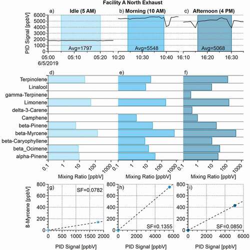
Panels g, h, and i of Figure 1 show an example of this process for the compound beta-myrcene. The panels in Figure 1 illustrate the data from the north exhaust of Facility A. The PID concentrations during sampling are seen as the line plot, with the shaded box indicating the tube sampling time period. Also included are the average PID values observed during the time tube samples were being taken. Panels d, e, and f show the speciated mixing ratios obtained from the tube sample for each time period.

• (3) Once the scaling factors were determined for each compound at each sampling time, the week-long PID data was then averaged from one-minute intervals to 15-min intervals to reflect the 15-min sample times at the first facility. It should be noted here that although different sampling times were used at the other facilities (5 and 10 min) we continued to use 15-min intervals for averaging the PID data at all sites. Calculation of the 5, 10, and 15-min averages at the other facilities indicated that there was a negligible difference in the overall emission factors calculated when using any of those averaged concentrations, so the decision was made to move forward using 15-min averages. This was also done to keep consistency with how the PID data was handled throughout the project. Each 15-min average point was then assigned to a bracketed time interval as described next.

• (4) Sampling time brackets were created based on inspection of the PID data. The brackets were picked based on the time the tube sample was taken, and the individual facility’s activity at that time. For instance, at Facility A, three different rounds of samples were taken (5:00 a.m., 10:00 a.m., and 4:00 p.m.). The data brackets created for this facility are labeled as the 5:00 a.m., 10:00 a.m., and 4:00 p.m. brackets. The 5:00 a.m. bracket reflects facility concentrations during the idle activity period (little to no staff in building, no product/plant activity taking place). Data assigned to this bracket included the PID values from 7:00 p.m. to 7:00 a.m. for Facility A. The 10:00 a.m. bracket includes data from 7:00 a.m. to 1:00 p.m., which includes the routine daily start-ups, harvesting and processing activities at Facility A. The 4:00 p.m. bracket includes data from 1:00 p.m. to 7:00 p.m., reflecting the end of the daily activities and clean-up processes at Facility A. This process can be seen in panel (a) of Figure 2.

Figure 2. Example determination of weekly extrapolated β-myrcene emissions from data collected at the Facility A north exhaust.

Panel (a) shows data from the photoionization detector (PID) at 1-min time resolution (green shaded) and 15-min averages (black circles). The gray shaded areas represent the hours, within a 24-hr period, that the β-myrcene response factor (see Figure 1) was multiplied by the 15-min average PID to extrapolate β-myrcene emissions over the entire week, as shown in panel (b). The average weekly extrapolated β-myrcene mixing ratio is also shown on panel (b).

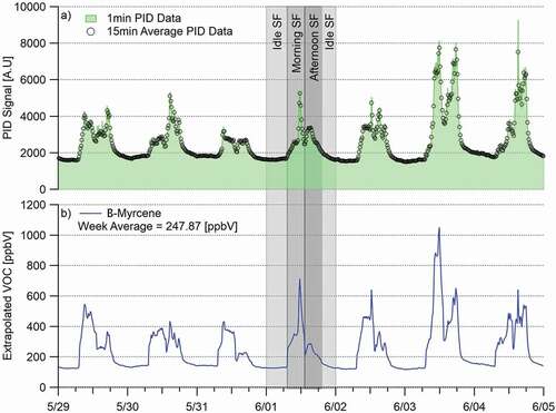
Facilities A and B were bracketed into three separate groupings based on the criteria mentioned above since three different samples were taken during the day. Facility D was bracketed into only two groups as there were only two time periods during which samples were collected. As Facility D was a medium-scale growth with carbon filters in place, it was decided to treat this facility as having one type of regular daily activity with a period of no activity instead of categorizing the daily activity into two levels as with Facilities A and B. Bracket times were slightly different at each facility based on the individualized sample plans used at each.

• (5) Once all the 15-min average PID points were assigned to an appropriate activity bracket, the normalized concentrations for the speciated tube data were calculated for the entirety of the week-long PID signal. This was accomplished by multiplying each 15-min PID data point value by the scaling factor associated with each compound during each bracketed time interval. An example of this process using the compound β-myrcene is seen in panel (b) of Figure 2. The equation used for this was:

(3) $\mathbf{C}{\mathbf{n}}_{\mathbf{A}}=\mathbf{P}\mathbf{I}{\mathbf{D}}_{\mathbf{15}}\times \mathbf{S}{\mathbf{F}}_{\mathbf{A}}$(3)

Cn_A: normalized concentration of compound A

PID₁₅: 15-min averaged PID data point, and

SF_A: scaling factor for compound A from appropriate time bracket

• (6) After the speciated tube data were scaled to the week-long PID signal, a weekly average was taken for each individual compound. Assumptions made during this step are that the overall makeup of the terpene compounds in the exhaust samples was not going to change as different strains are processed through the facility, and that the facility’s activity levels would remain consistent throughout the year. This is not actually the case, as different plant strains have different terpene profiles. This study is merely a snapshot of the concentrations seen on one or two days of the year at each facility and is highly dependent on the strains growing or being harvested or processed on that day.

• (7) The normalized weekly average concentrations for each compound were converted from ppb to micrograms per cubic meter.

• (8) This value was then converted to an estimated emission value (E) of micrograms per week (mg/week) by multiplying it with the total exhaust air flow volume in equation (4) (in cubic meters per week, Table S2 in the supplemental documents). The values were subsequently transformed into micrograms per year by multiplying by 52 weeks per year, and then into pounds per year by multiplying by the conversion by 1 microgram equals 2.2 × 10⁻⁹ pounds.

(4) $\mathbf{E}=\mathbf{C}{\mathbf{n}}_{\mathbf{A}}\times \mathbf{F}\mathbf{v}$(4)

E: Emission rate (mg/week)

Cn_A: Concentration (mg/m³)

Fv: Flow volume (m³/ week)

• (9) The pound per year values were then summed up to provide an overall total for the exhaust point. In the case of Facility A, two emission values were obtained, one for the north exhaust and one for the south. These values were then summed to provide a total terpenes emission value for the facility. At Facility B, there was only one exhaust point, but sampling was performed on two different occasions, so the values obtained from each day of sampling were averaged to provide a facility total. The calculations for Facility D were slightly more complex with the two exhaust points in that the values obtained for the front exhaust with the door both open and closed were averaged together to provide a single value for the front exhaust. This value was then added to the value obtained for the rear exhaust to provide a facility total for terpene emissions.

Calculation uncertainties

Calculation uncertainties are due to a number of factors. These include:

• Assuming zero tube concentrations when the PID signal is zero.

• Assuming PID signal obtained is due only to the compounds measured with the tubes.

• Inaccurate measurements of flow, temperature, and pressure in the exhaust systems.

• Assuming activity brackets and subsequent value assignments are the same from day to day.

Ozone modeling methods

Ozone modeling was performed by Ramboll US Consulting, Inc for the DM/NFR ozone NAA for the 2016 summer ozone season and was used as a base case (Ramboll 2020). The results of this sampling study were used to perform additional modeling specifically to assess if there are impacts on ozone formation due to cannabis VOC emissions. For both the base case and the additional simulations, ozone was modeled using a photochemical grid model (PGM). PGMs are computer models used to simulate changes in pollutant concentrations for particular locations using complex physical and chemical mathematical equations. Model inputs include meteorological data and gridded emissions data based on anthropogenic and biogenic emission inventories. Model outputs include gridded ozone and fine particulate matter (PM_2.5) concentrations. The PGM modeling was conducted using the same 2016 PGM modeling platform as used in the ozone attainment demonstration modeling for the DM/NFR NAA Serious ozone State Implementation Plan (SIP) under the 2008 ozone NAAQS. The base case simulation was subject to a model performance evaluation to establish the reliability of the base case modeling for predicting MDA8 ozone and related concentrations. The evaluation compared the base case model estimates against observed ambient MDA8 ozone concentrations and assessed the ability of the model’s air quality predictions to correctly respond to changes in emissions and meteorology. Details on the 2016 PGM modeling platform development and model performance evaluation are provided in the Serious ozone SIP 2016 base case modeling report (Ramboll 2020a) and Air Quality Technical Support Document (AQTSD; Ramboll 2020e). Three simulations were conducted:

1. Base case using 2016 actual emission data without emissions from cannabis cultivation;

2. Average cannabis case that added cannabis cultivation VOC emissions to the 2016 base case determined from the average study emission factors; and

3. High cannabis case that added cannabis cultivation VOC emissions to the 2016 base case based on the highest study emission factor.

The 2016 base case model was used to assess the impact of adding cannabis cultivation VOC emissions. Model results with and without cannabis emissions were compared for assessment of increases in modeled ozone MDA8 values resulting from the added cannabis VOC emissions (Ramboll 2020).

Model selection

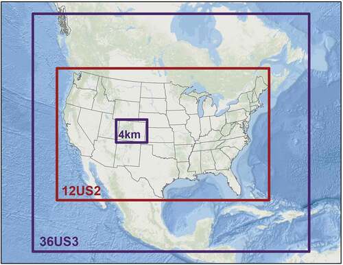
Ramboll US Consulting, Inc. used the Comprehensive Air-quality Model (CAMx 2021) PGM to simulate ozone and PM_2.5 concentrations across nested 36/12/4-kilometer (km) modeling domains, shown in Figure 3, for May through August 2016. May 2016 was used as a model initialization period using just the 36-km modeling domain for computational efficiency, with the full 36/12/4-km domain configuration started on June 1. The domains utilized two-way interactive grid nesting with boundary conditions for the 36-km domain based on output from the GEOS-Chem global chemistry model. The PGM modeling platform used the same 36-km 36US3 and 12-km 12US2 domains used in the final (EPA 2016) modeling platform (2016v1) (EPA 2016). A 4-km grid resolution domain covering Colorado was added to the 36/12-km domain structure. The CAMx model vertical grid included 35 layers from ground level to 50 mb (approximately 17,500 m above ground level).

Figure 3. Air quality modeling domains used for CAMx (Ramboll 2019a).

The 36US3 (36-km) and 12US2 (12-km) gridded domains are the same as used in the EPA 2016v1 platform. The 4 km Colorado domain is from the DM/NFR Serious Ozone State Implementation Plan’s (SIP) photochemical modeling demonstration (Ramboll 2020).

Inputs to CAMx were developed using several tools. Meteorology was modeled using the Weather Research Forecast (WRF) prognostic meteorological model (NCAR 2021). Model-ready emission data were generated using the Sparse Matrix Operator Kernel Emissions (SMOKE) model (CMAS 2019). Biogenic emissions were modeled using the Model of Emissions of Gases and Aerosols from Nature (MEGANv3.1) (UCI 2019). CAMx pre-processors were used for windblown dust (WBD), lightning NOx (LNOx), sea salt (NaCl), and dimethyl sulfide (DMS) emissions. The 2014 version of the Motor Vehicle Emissions Simulator (MOVES2014b) on-road mobile source emission model was used with SMOKE-MOVES and 2016 WRF meteorological data to generate on-road mobile source emissions (EPA MOVES 2020b). Link-based vehicle activity data within the DM/NFR NAA was used at the county level.

Model data inputs

Meteorological inputs to CAMx were based on EPA’s 2016 36/12-km WRF simulation with the 4-km Colorado domain meteorology interpolated from the 12-km resolution data using the CAMx flexi-nest feature. Boundary conditions for the 36-km 36US3 domain were based on a 2016 simulation using the GEOS-Chem global chemistry model (Harvard 2021). The GC2CAMx processor was used to generate day-specific diurnally varying boundary conditions extracted from GEOS-Chem to define the lateral boundaries around the 36-km 36US3 modeling domain.

CAMx requires model-ready emission data consisting of hourly emissions of specific gas and particle species for the horizontal and vertical grid cells within the modeling domain. The 2016 base case emission data were based on the EPA 2016v1 emission estimates (EPA 2016). For the 4-km Colorado domain, CDPHE APCD updates for Colorado oil and gas and on-road mobile sources were used. New emissions were generated for natural emission sources, including biogenic and LNOx for all three domains (Ramboll 2020a). The 2016 EPA platform used the BEIS biogenic emission model (EPA 2020a). These emissions were replaced by MEGAN biogenic emissions in all three domains (UCI 2019). Monthly emission inventories were processed using SMOKE to provide speciated emission data and to spatially allocate emissions both laterally and vertically to grid cells and temporally to day-of-week and hour-of-day. The base case simulation did not include cannabis cultivation emissions. Two simulations were run with cannabis cultivation emissions added to the base case emission inventory; a high emission scenario and an average emission scenario.

Cannabis emission inventory development and processing

Sampling data and cannabis harvest data for 2019 were used to generate a VOC emission inventory for cannabis grow operations in Colorado. A ratio of measured VOC in the cultivation facility exhaust streams and the total harvested plant weight was used to calculate a VOC emission factor (EF) for each facility. Table 3

Table 3. Cannabis cultivation VOC emission factors.

Facility	Terpene emissions (lbs/year)	Harvested plant weight (tons/year)	VOC EF (lbs terpenes/ton harvested plant weight)
Facility A	1,417 ± 452	127	11.12 ± 3.56
Facility B	385 ± 121	180	2.13 ± 0.67
Facility D	105 ± 55	23	4.51 ± 2.39
Average EF	–	–	5.92 ± 2.51

shows the calculated emission factors for the three study facilities in terms of pounds (lbs) of VOC emitted per ton of harvested plant weight.

The emission factors were used to develop an emission inventory for two modeling scenarios, a high emission scenario and an average emission scenario. The high emission scenario was based on the emission factor for Facility A, the highest EF among the three facilities. The average emission scenario was based on the average VOC EF for the three facilities that exhaust samples were collected from.

An emission inventory for each scenario was built based on the emission factor and the commercial cannabis cultivation facility biomass production for each county from 2019 MED data. The locations of cultivation facilities in 2019 are shown in Figure 4. In some cases, production data were only available for a group of counties instead of a single county. For those counties, the total harvested plant weight was divided by the number of facilities in the affected counties, then apportioned to each county by the number of facilities in that county. Equation (3) is used to calculate emissions and build a county-level inventory in terms of tons of VOC per year for each of the two scenarios.

(5) $VOC=EF\left(\frac{lbs}{ton}\right)\ast Wetweightofharvest\left(\frac{tons}{year}\right)(\frac{tons}{year})\ast 0.0005\left(\frac{tons}{lb}\right)$(5)

Figure 4. Location of 2019 active cannabis cultivation facilities in Colorado (Ramboll 2020).

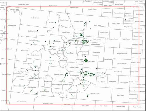
The cannabis emission inventories were estimated and processed using SMOKE to generate hourly gridded speciated emission inputs that were merged with the rest of the 4-km Colorado domain emissions. SMOKE uses spatial surrogates to distribute emissions laterally to modeling grid cells. These surrogates were developed for cannabis cultivation facilities by overlaying the 4-km modeling domain on a map of the facility locations with their latitude/longitude coordinates. Vertical allocation to grid cells assumed new cannabis emissions were released into layer 1 of the CAMx modeling domain, up to approximately 20 m above ground level. While cultivation facilities are considered point sources, the PGM models do not explicitly resolve point source plumes. Point source emissions were distributed into a 4-km grid cell. Due to data confidentiality issues, the location data did not include associated production data. Therefore, marijuana production rates and subsequent emissions were assumed to be equally distributed among facilities within a given county.

The data collected at each facility were used to develop a chemical speciation profile for the CB6r4 photochemical mechanism used in the CAMx modeling. This profile showed 98.8% by weight of cannabis emissions were terpenes (TERP) and 1.2% by weight were sesquiterpenes. Atmospheric chemistry consists of millions of reactions among many thousands of chemical compounds. Condensed chemical mechanism is an integral part of the photochemical modeling and cannot address individual species reactivities.

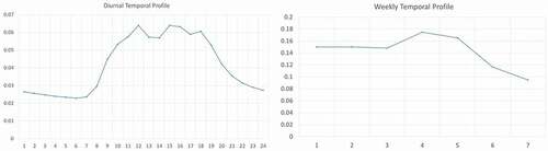
The study included a week-long period of 1-min PID data for each of the three study facility’s exhaust points. This data was used to develop weekly and diurnal temporal profiles to allocate monthly emissions to day-of-week and hour-of-day. The profile showed that emissions were larger when workers were working in the building from 8am-6pm Monday through Friday and lower outside of working hours. The profile also showed increased emissions toward the end of the week, which is consistent with an operational practice of harvesting more toward the end of the week. The weekly and diurnal temporal profiles are shown in Figure 5.

Figure 5. Weekly and diurnal temporal profiles for cannabis emission (Ramboll 2020).

Air modeling uncertainties

The VOC emission increase due to commercial cannabis cultivation is very small and the analysis of the model results took the difference between two model simulations, a base case and two cannabis emission scenarios. Thus, there is a potential for model noise to be of a comparable magnitude to the difference between ozone or PM_2.5 concentrations in the simulations. Model noise refers to changes in ozone or PM_2.5 concentrations between the two simulations that are not directly related to the changes in emissions being analyzed. Model noise can occur due to round-off errors in the calculations. Another potential source of model noise is if the numerical algorithms in the solutions of the differential equations use branching and extremely small changes that cause the numerical algorithm to take two different branch solutions that cause a higher concentration change than there should be. The ISORROPIA aerosol thermodynamic module is especially susceptible to causing model noise in ammonium nitrate PM_2.5 concentrations (Miami ISORROPIA II 2007).

Difference plots in the maximum daily average 8-hr (MDA8) ozone and 24-hr PM_2.5 concentrations between the cannabis scenarios and the base case were examined to determine whether the model noise comparable to the ozone impacts of the cannabis VOC emissions occurred. Model noise is usually indicated by patches of pixelated differences of adjacent grid cell increases and decreases in the spatial difference plots. For the ozone modeling, possible model noise was detected during July 6–10, 2016, so those five days were eliminated from the analysis. For PM_2.5, possible model noise was detected on June 19, 2016, and in additional days that were also eliminated from the analysis (Ramboll 2020).

Although model noise was detected on some days of the modeling, through elimination of those days in the analysis, the results presented are believed to be reliable and represent real calculated impacts of the effects of cannabis cultivation VOC emissions on ozone and PM_2.5 concentrations.

Results

Pilot study

The Pilot Study results determined that SUMMA® canisters proved to be a less viable option than the Tenax tubes for quantifying cannabis terpenes due to the “sticky” nature of the semi-volatile terpenes and terpenoid compounds. Terpene compounds can adhere to the canister walls after sampling, making it difficult to extract them from the canisters for lab analysis. The Tenax tubes proved to be a more reliable sampling media for that same reason–the terpenes were efficiently trapped within the sorbent media inside the tubes, and subsequently thermally desorbed for the lab analyses in a more effective manner.

The pilot study results provided an indication of what concentration levels to expect, how well the instrumentation captured the VOC profile, and the best way to approach future sampling. The SUMMA® canister results indicated low isoprene concentrations and other VOCs relative to the total mass of monoterpenes, which resulted in the decision not to use them in the remainder of the project. During the pilot study, DRI researchers estimated that the monoterpenes contributed 86% to 99% of the total VOC mass. The pilot study also revealed the presence of other sources of VOCs in addition to the plant terpenes in the form of cleaning/sterilization solvents. Emissions from these compounds were not accounted for in this study as we were focused on the plant-based emissions. Solvent emissions for facilities can be estimated based on annual purchases and/or permit requirements. While Summa canisters are effective at collecting and quantifying VOCs in the C1 to C10/11 range, Tenax tubes are effective at collecting them in the C6/7 to C26 range. Many of the solvents used in the facilities were alcohol based, and in the C1 to C3 range. Using the Tenax tubes instead of the Summa canisters for the analyses lowered the necessity of accounting for solvent concentrations because they were not retained on the tubes’ sample medium, though they are picked up in the PID signal.

Main study

Table 3 shows the calculated emission factors for the three study facilities in terms of pounds (lbs) of VOC emitted per ton of harvested plant weight. To obtain the emissions factors used in the model, the terpene emissions in pounds per year were divided by the harvested wet plant weight. Standard deviations were calculated from the weekly average compound concentrations that were scaled from the total VOC signal of the PID. The VOC emission factor for facility A is much higher than the others due to the Facility’s HVAC design having over 20 times the exhaust volume of facility B as demonstrated in Table S2 in the supplemental documents and a larger amount of plant weight harvested as shown in Table 3.

Annual emissions for the high, average, and low estimated VOC emissions are shown in Table 4. These values were obtained using the VOC EF values in Table 3, multiplying them by the total wet weight of the plant harvest statewide and in the NAA (in tons, obtained from 2019 marijuana harvest information from the Department of Revenue), and finally by a conversion factor, as in equation 5. There were 1,167 grow facilities in Colorado, and 589 in the NAA according to the Marijuana Enforcement Division. To obtain a possible range of annual emissions statewide and in the NAA (in TPY), the highest and lowest emission rates from Table 4 were multiplied by 1,167 (statewide) or 589 (NAA) to calculate possible high and low VOC emissions for both in tons per year (TPY). These calculations provide an estimated range of 5,401 to 28,196 total TPY for the state, and 1,722 to 8,933 total TPY for the NAA. As the wet weights were calculated on a county-wide basis, the 9-county DM/NFR NAA VOC emissions include the full counties, not just the portions within the NAA boundary. The distribution of commercial cannabis cultivation facilities is shown in Figure 4. The statewide range values are much smaller than those found in the Wang et al. study, which found a biogenic VOC emission rate of 340,268 metric TPY (375,081 US tons) statewide (Wang et al. 2018). For the NAA, Wang calculated a biogenic VOC emission rate of 265 metric TPY (292 US tons), which is much smaller than the range calculated in this study (Wang et al. 2018). The large differences are due to each study’s sampling methodology and assumptions made.

Table 4. Estimated cannabis cultivation VOC emissions as terpenes in tons per year.

	VOC emissions in tons of terpenes/year
Region	High	Average	Low
State-wide	24.2 ± 7.7	12.9 ± 5.5	4.6 ± 1.5
9-county DM/NFR NAA	15.2 ± 4.9	8.1 ± 3.4	2.9 ± 0.9

The five dominant terpenes at Facility A were β-caryophyllene, D-limonene, terpinolene, β-myrcene, and α-pinene respectively. The five dominant terpenes at Facility B were β-caryophyllene, D-limonene, α-pinene, terpinolene, and ɣ-terpinene, respectively. The five dominant terpenes at Facility D were β-caryophyllene, terpinolene, D-limonene, β-myrcene, and α-pinene respectively. Terpene concentrations can be seen in Table S3 in the supplemental documents section.

Air modeling results

Ramboll US Consulting, Inc. conducted three CAMx simulations for the May–August 2016 ozone season using the CAMx 36/12/4-km base case configuration. Ozone and PM_2.5 results were reviewed based on the averaging times in their respective NAAQS. For ozone, this was the MDA8 ozone concentration, and for fine particulate matter, this was the maximum 24-hr PM_2.5 concentration. The CAMx output for the average and high emission cases were compared to the base case. The contribution of cannabis cultivation emissions to ozone and PM_2.5 was obtained by taking the difference between the modeling results for the base case and each of the two cannabis simulations (average and high) (Ramboll 2020).

Ozone impacts

The increase in VOC emissions due to the addition of the high and average cannabis cultivation VOC emissions was very small. The largest concentration of cannabis cultivation facilities is located in the DM/NFR NAA and the addition of the high and average cannabis VOC emissions represented an increase in VOC emissions of only 0.009% and 0.005%, respectively, across the 9-county DM/NFR area (Ramboll 2020).

The majority (98.8%) of the cannabis VOC emissions are terpene species represented by the TERP species in the CB6r4 chemical mechanism used in the CAMx simulations. Condensed chemical mechanism is an integral part of photochemical modeling and cannot address individual species reactivities. These species can participate in photochemistry to form ozone in the presence of sunlight with other VOC species and NOx. These species can also react directly with ozone resulting in reduced ozone concentrations when photochemistry is low or non-existent (Ramboll 2020). Table 5 shows the total 2016 base case VOC emissions in the nine counties of the DM/NFR NAA and the additional VOCs included in the high and average cases.

Table 5. Estimated cannabis VOC comparison to 2016 VOC emissions in 9-county DM/NFR.

Scenario	VOC in tons/day			% Increase
	Biogenic	Anthropogenic	Total
2016 Base Case	178.68	367.99	546.68	–
Cannabis High	–	0.05	546.73	0.009
Cannabis Average	–	0.03	546.71	0.005

a(includes northern Larimer and Weld Counties), in tons per day (Ramboll 2020).

Ozone impacts were evaluated by comparing differences in MDA8 ozone concentrations. The highest MDA8 ozone concentration in each simulation for each grid cell for the June–August 2016 modeling period was identified. The difference between the highest base case MDA8 ozone concentration and the highest cannabis scenario MDA8 ozone concentration was calculated for each grid cell and for each of the cannabis scenarios. The highest base case and cannabis scenario MDA8 concentration could have occurred on different days. Increased ozone concentrations were seen in Denver County, portions of counties adjacent to Denver County, and along the Larimer and Weld County border. The largest maximum MDA8 ozone increase for the high and average cannabis scenarios, respectively, was 0.011 and 0.006 parts per billion (ppb) ozone and was seen in the southwest corner of Denver County (Ramboll 2020). The cannabis scenarios also showed slight decreases in the highest MDA8 ozone concentrations in the eastern portions of Adams and Weld Counties in the DM/NFR and in Park, Clear Creek, and Grand Counties to the west of the DM/NFR. The results for the two cannabis scenarios are shown in Figure 6.

Figure 6. Differences in highest MDA8 ozone concentrations.

L = Larimer County, GR = Grand County, B = Boulder County, G = Gilpin County, CC = Clear Creek County, P = Park County, J = Jefferson County, D = Denver County, W = Weld County, AD = Adams County, AR = Arapahoe County, DG = Douglas County, E = Elbert County (Ramboll 2020).

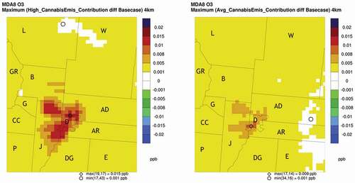
The largest differences in MDA8 ozone concentrations were also evaluated. For each day in the modeling period and for each grid cell, the difference between the base case MDA8 ozone concentration and each cannabis scenario MDA8 ozone concentration was calculated and the maximum difference for the modeling period was identified. For the high cannabis scenario, the largest MDA8 ozone difference was 0.015 ppb and occurred in the northern part of Denver County near Adams County. The average cannabis scenario had a maximum impact of 0.009 ppb and occurred in southwest Denver County near Jefferson County . There were three areas that showed an increase in the MDA8 difference, northern Denver County, southwest Denver County, and northern Jefferson County. These results are shown in Figure 7 (Ramboll 2020).

Figure 7. Largest ozone increases for differences in MDA8 ozone concentrations between the base case and cannabis scenarios.

L = Larimer County, GR = Grand County, B = Boulder County, G = Gilpin County, CC = Clear Creek County, P = Park County, J = Jefferson County, D = Denver County, W = Weld County, AD = Adams County, AR = Arapahoe County, DG = Douglas County, E = Elbert County (Ramboll 2020).

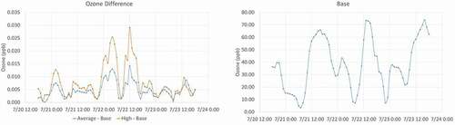
Model results were evaluated across the entire 4-km Colorado domain at the time and location of the highest differences in MDA8 ozone concentrations. The largest modeled difference in MDA8 concentrations occurred on July 22, 2016, and was 0.015 ppb for the high cannabis emission scenario. For the grid cell where the maximum difference occurred, a time series of hourly ozone concentrations for the base case and the two cannabis scenarios was reviewed for July 21–23, 2016, as shown in Figure 8. The base case total ozone at this grid cell was in the 60–70 ppb range. The peak hourly ozone concentration on July 22, 2016, at this location was 73 ppb occurring at 1:00 p.m. Mountain Standard Time (MST). The model results show two peaks on July 22 in the differences in hourly ozone between the cannabis cases and the base case. A 0.025 ppb difference occurred at 4:00 a.m. MST and a second 0.029 ppb peak occurred at 12:00 p.m. MST. The 4:00 a.m. peak appears to be remnants of the previous day’s ozone as photochemistry would not be occurring that early in the day. The second peak occurred at noon, which is earlier in the day than total hourly ozone concentration peaks occur (1:00 p.m. – 3:00 p.m.). This reflects the more VOC-limited photochemistry in the Denver urban areas in the morning and more NOx-limited photochemistry in the afternoon. Thus, cannabis VOC emissions produce more ozone in the morning than later in the day (Ramboll 2020).

Figure 8. Time series of hourly ozone concentrations on July 21–23, 2016, comparison of base case hourly ozone (bottom) and differences in hourly ozone for the high and average cannabis scenario (top) (Ramboll 2020).

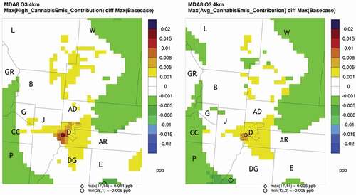
Ozone concentrations and the impact of cannabis VOC emissions across the Colorado 4-km domain were evaluated for four high-ozone days in the DM/NFR NAA. These days were June 21, July 25, August 3, and August 12, 2016. Base case ozone concentration and contributions from the high emission scenario and average emission scenario are shown in Table 6. On all four dates, the highest base case ozone concentration and the maximum cannabis contribution for both scenarios occurred in the DM/NFR NAA. On June 21, 2106, the highest base case ozone concentration was 76.7 ppb and occurred in the southeast corner of Larimer County. The highest MDA8 contribution due to the high cannabis emission scenario was 0.006 ppb and occurred just north of Broomfield County, slightly south of where the highest MDA8 ozone occurred in the base case. The highest MDA8 contribution due to the average cannabis emission scenario was 0.003 ppb and also occurred just north of Broomfield County. On July 25, the base case peak MDA8 ozone concentration of 70.4 ppb occurred at the border of Jefferson and Clear Creek Counties. The highest contributions due to the high and average cannabis VOC emissions were, respectively, 0.015 and 0.009 ppb and occurred in the northeast corner of Denver County. The peak MDA8 ozone concentration on August 3 was 83.6 ppb and occurred in central Jefferson County. The highest contributions due to the high and average cannabis VOC emissions were, respectively, 0.006 and 0.004 ppb and occurred in Adams County just north of Denver. On August 12, the base case MDA8 ozone peak was 74.8 ppb and occurred in Jefferson County just west of Denver County. The maximum contributions of the high and average cannabis scenarios were, respectively, 0.005 and 0.002 ppb and occurred near the base case peak location. It is recognized that more sensitivity runs and scenario variations could be modeled but due to time and budget constraints this study focused on modeling just the high and average scenarios as the main focus was the impact that the cannabis industry has on ozone formation in the DM/NFR NAA (Ramboll 2020).

Table 6. High and average scenario cannabis contributions to ozone (Ramboll 2020).

Date	Base ozone (ppb)	High scenario ozone (ppb)	Average scenario ozone (ppb)
June 21, 2016	76.7	0.006	0.003
July 25, 2106	70.4	0.015	0.009
August 3, 2016	83.6	0.006	0.004
August 25, 2016	74.8	0.005	0.002

PM_2.5 impacts

Cannabis VOC emissions can increase fine particulate matter concentrations through two main pathways. Cannabis emissions are mostly terpenes with a small amount of sesquiterpene. Both terpenes and sesquiterpene are precursors to Secondary Organic Aerosol (SOA) PM_2.5. Cannabis VOCs can also participate in photochemistry that can convert gaseous species into secondary PM_2.5 such as sulfate and nitrate (Pye et al. 2010, 2019). The first of these two pathways is believed to be more important as the cannabis VOCs are a small portion of total VOCs in the state.

In the CAMx model, TERP reacts with hydroxyl radical (OH) to form a condensable gas (CG) that is in thermodynamic equilibrium with particulate SOA. Cool moist conditions favor particulate SOA and hot dry conditions favor CG. Since a summer period was modeled, the equilibrium would favor the CG. This may result in an underestimation of the maximum PM_2.5 concentrations that will form during the year.

There are two PM_2.5 NAAQS; one is a 24-hr standard with a threshold of 35 µg/m³, and the other is an annual standard with a threshold of 12 µg/m³. Since only the summer of 2016 was modeled, the impact of cannabis emissions on PM_2.5 was evaluated by comparing maximum 24-hr PM_2.5 concentrations in the base case and the two cannabis scenarios. Differences in the highest 24-hr concentrations and the highest differences in 24-hr concentrations were evaluated, in the same manner as for ozone. The highest 24-hr PM_2.5 concentrations in each simulation for the June–August 2016 modeling period were compared. The highest 24-hr PM_2.5 concentration in each grid cell for each scenario was identified, and the difference between the base case and each cannabis scenario was calculated. The high cannabis scenario produced increases of 0.001 µg/m³ or higher in the highest 24-hr PM_2.5 concentrations. The highest increases in PM_2.5 concentrations due to the high and average cannabis scenarios are, respectively, 0.004 and 0.002 µg/m³ (Ramboll 2020).

The largest difference in maximum 24-hr PM_2.5 concentrations was selected in each grid cell across the days in the modeling period. For the high and average cannabis scenarios, the largest maximum 24-hr PM_2.5 difference was, respectively, 0.009 µg/m³ and 0.005 µg/m³ (Ramboll 2020).

Overall study uncertainty

Uncertainties for each step in the process are reported in the method section. In general, the analytical and laboratory uncertainties are less than 40%. The uncertainty is estimated based on the variability in the sampling and analytical equipment, the assumptions of (1) a linear response of the PID to individual terpene compounds, (2) consistent facility activity brackets, and (3) no interference from non-terpene based VOC sources (the PID signal is due only to the terpenes being measured). Modeling uncertainty is generally based on the assumptions made and is therefore larger than analytical uncertainty. For example, representative VOC reactivities are used for monoterpenes, terpenoids, and sesquiterpenes, rather than compound-specific reactivities. While this is unlikely to affect the results of the analysis in a significant way, the relative error is greater than that of the analytical uncertainty. In addition, many assumptions have been made in the calculation of the emission factors, such as assuming zero tube concentrations when the PID signal is zero for creation of the scaling factors, assuming the PID signal is due solely to the VOCs measured via the tube samples, and assuming that activity levels and species grown are the same throughout the year. The dominant uncertainty in this analysis is the variability between facilities in terms of processes, staffing, operational methods, strains grown, and exhaust methods. Collectively, these are, by far, the largest sources of uncertainty in this effort. We collected samples at three very different facilities, all typical for the industry in Colorado and averaged their emission factors to mitigate this uncertainty. However, there is no way to quantify this uncertainty definitively. With that in mind, the results of modeling show that terpenoid emissions would have to be orders of magnitude larger to have a significant effect on ozone formation in the DM/NFR NAA.

Comparing results to previous study results

The dominant terpenes from this sampling study present in most samples were β-caryophyllene, D-limonene, terpinolene, α-pinene, β-pinene, and β-myrcene, respectively, by concentration. DRI’s (Samburova et al. 2019) study found β-myrcene, D-limonene, terpinolene, α-pinene, and β-pinene to be the dominant terpene emissions from cannabis, which is also consistent with the results of this study. The DRI Truckee study also found α-pinene to be a dominant terpene emitted from cannabis (Samburova et al. 2019). Our study was also in alignment with the results of Wang et al. (2019), which identified β-myrcene and d-limonene as dominant terpenes emitted from cannabis with the addition of eucalyptol and γ-terpinene. This sampling study did also result in notable amounts of eucalyptol and γ-terpinene emissions from Facility B but only trace levels at Facility A and D, which is most likely attributed to the unique strains grown at the facility. Ross and ElSohly (1996) also found β-myrcene and limonene to be dominant terpene emissions from cannabis, which is in alignment with our study. Overall, the dominant terpenes in the samples collected for this study were similar to previous study findings with the exception of high levels of β-caryophyllene that the other studies did not find. Table 7 shows the values for some of the top compounds seen in this and other studies. The differences in terpene concentrations between this study and other studies can be attributed to the diversity of cannabis strains grown at each facility, operational parameters, and sampling methodology.

Table 7. Comparing terpenes concentrations to previous studies.

Study	(μg/m^3)
	β-myrcene	Terpinolene	α-pinene	β-pinene	Δ-limonene
CDPHE, weekly avg scaled concentration	1381 ± 830	188 ± 178	78 ± 39	53 ± 10	433 ± 206
Samburova et al. 2019 (cure room)	840 ± 96	312 ± 23	1036 ± 124	3766 ± 452	202 ± 12
Study	ppbv
	β-myrcene	Terpinolene	α-pinene	β-pinene	Δ-limonene
CDPHE, weekly avg scaled concentration	248 ± 149	34 ± 32	14 ± 7	10 ± 5	78 + 37
DRI-Washoe, 2016 (max of canister samples)	909 ± 17	329 ± 6	168 ± 9	95 ± 2	232 ± 10
DRI-Truckee, 2014 (canister sample)			3.6

Conclusion

Cannabis cultivation terpene emissions

Based on our sample results and calculated VOC emission rates, overall cannabis emissions are a very small percentage of total biogenic and anthropogenic VOC inventory in the DM/NFR NAA. The cannabis cultivation terpene emissions account for less than 0.01% of total VOC in the DM/NFR NAA (Ramboll 2020). A vast majority (~99%) of the cannabis VOC emissions are terpene species with the remainder being sesquiterpene.

Ozone impacts of cannabis VOC emissions

Given that the cannabis VOC emissions are a small fraction of the total VOC emissions in the DM/NFR NAA, it is not surprising that the ozone impacts are also very small. The largest change in the mean MDA8 ozone concentrations in the high and average cannabis VOC emission scenarios were, respectively, 0.015 and 0.009 ppb (Ramboll 2020). Most of the time, the largest increase in MDA8 ozone due to the cannabis VOC emissions occurred in Denver County or nearby. The ozone impacts of the cannabis emissions were small and below what is routinely reported in ozone observations.

PM_2.5 impacts of cannabis VOC emissions

The highest increases in 24-hr PM_2.5 concentrations due to the high and average cannabis scenarios were, respectively, 0.009 and 0.005 µg/m³ (Ramboll 2020). Like for ozone, these PM_2.5 increases are also very small and below what is routinely reported in PM_2.5 observations.

Overall conclusion

This study concluded that even though cannabis cultivation facilities can have overwhelming nuisance odor impacts, based on samples collected and production rates they actually have a low VOC emission rate (2.13 to 11.12 lbs of VOC/ton of cannabis harvested), even at large high-volume production facilities. Additionally, the dominant VOC emissions from samples collected at the three cannabis cultivation facilities were β-caryophyllene, D-limonene, terpinolene, α-pinene, β-pinene, and β-myrcene, terpenes common to many other types of trees and plants (Fischedick et al. 2010; Fuentes et al. 2000; Marchinia et al. 2014; Ross and ElSohly 1996; Samburova et al. 2019; Sharkey et al. 2008; Turner et al. 1979; Wang et al. 2018). It is interesting to note that the emission profile lacked isoprene, a terpene commonly emitted from other plants that is highly reactive for ozone formation (Sharkey et al. 2008). The resulting low VOC emission rate and the lack of isoprene from cannabis cultivation facilities sampled resulted in a very low to negligible impact on both ozone (0.005–0.009% increase in ozone from cannabis cultivation) and PM_2.5 formation (largest maximum 24-hr PM_2.5 difference of 0.009 µg/m) in the DM/NFR NAA (Ramboll 2020). Given the potentially large uncertainties and variability in cultivation facilities coupled with a small sampling budget and specific ozone model inputs, the resulting cannabis VOC emissions could vary widely in different areas of the country based on many industry variables such as cultivation methodology, location, production rates, strains grown, ambient air chemistry, local weather, proximity to other industries, etc. Further sampling and research could help refine the VOC emissions rate and speciation of cannabis.

Data availability

PID data are available on request from CDPHE.

Acronym Glossary

APCD	=	Air Pollution Control Division
BEIS	=	Biogenic Emission Inventory System
BER	=	basal emission rate
CAMx	=	Comprehensive Air-quality Model
CDPHE	=	Colorado Department of Public Health and Environment
CG	=	condensable gas
DM/NFR	=	Denver Metro North Front Range
DMS	=	dimethyl sulfide
DRI	=	Desert Research Institute
EF	=	Emission Factor
EPA	=	U.S. Environmental Protection Agency
HVAC	=	Heating, ventilation, and air conditioning
I.D.	=	inner diameter
km	=	kilometer
L	=	liter
lbs	=	pounds
LNOx	=	lightning NOx
m	=	meter
mm	=	millimeter
MDA8	=	maximum daily average 8-hour
MDL	=	minimum detection limit
MED	=	Colorado Department of Revenue’s Marijuana Enforcement Division
MEGAN	=	Model of Emissions of Gases and Aerosols from Nature
MIP	=	Marijuana Infused Product
MOVES	=	Motor Vehicle Emissions Simulator
MST	=	Mountain Standard Time
NAA	=	Nonattainment Area
NAAQS	=	National Ambient Air Quality Standards
NaCl	=	sea salt
NOx	=	Oxides of Nitrogen
OH	=	hydroxy radical
PGM	=	photochemical grid model
PID	=	photoionization detector
PM	=	Particulate Matter
ppm	=	parts per million
ppb	=	parts per billion
ppbv	=	parts per billion by volume
SOA	=	Secondary Organic Aerosol
SIP	=	State Implementation Plan
SMOKE	=	Sparse Matrix Operator Kernel Emissions
TPY	=	Tons per Year
µg	=	micrometer
µg/m3	=	micrometers per cubic meter
VOC	=	Volatile Organic Compound
WBD	=	windblown dust
WRF	=	Weather Research Forecast

Acknowledgment

The authors want to acknowledge the time and efforts of the cooperating volunteer cannabis cultivation facilities throughout this study.

The authors also thank Jason Schroder, Daniel Bon, Kevin Briggs, Kira Shonkwiler, and Dale Wells of CDPHE, William Vizuete and Chi-tsan Wang of the University of North Carolina, Tejas Shah and Ralph Morris of Ramboll U.S. Consulting, Inc., Chiranjivi Bhattarai, Irina Lebedeva, and Vera Samburova of Desert Research Institute, Christine Wiedinmyer of the University of Colorado in Boulder, Michael Wolf of Washoe County Air Quality, and Joe Southwell of Spokane Regional Clean Air Agency, Greg Harshfield, Alex Neibergall, and Anando Mukherjee previously of CDPHE for their scientific inputs that helped inform this study and publication.

The authors also thank CDPHE management staff for their ongoing support of this study. Specifically, Garry Kaufman, Dena Wojtach, Gordon Pierce, Leah Martland, and Emmett Malone. Thanks to the 2018 CDPHE Innovation Grant for funding for this study.

Disclosure statement

No potential conflict of interest was reported by the author(s).

Supplementary material

Supplemental data for this paper can be accessed on the publisher’s website

Additional information

Funding

This work was supported by the Colorado Department of Public Health and Environment.

Notes on contributors

Kaitlin Urso

Kaitlin Urso is an environmental consultant with the Colorado Department of Public Health and Environment that specializes in helping small businesses reduce their environmental impacts and comply with regulations. Kaitlin was the lead author and project engagement manager for this study on cannabis air emissions and impacts. She has 11 years of technical environmental experience and a mechanical engineering degree from the University of Colorado. Kaitlin's work has been featured in Wall Street Journal, Forbes, CNN, NPR, Science Magazine, and countless other media publications.

Alicia Frazier

Alicia Frazier is a physical scientist with the Colorado Department of Public Health and Environment’s Air Pollution Control Division. She specializes in planning and performing a variety of air toxics sampling activities. Alicia designed and implemented the sampling process, and established the emissions factor calculations for this study on cannabis air emissions and impacts. She has over 20 years of environmental sampling experience, and a M.S. in Astrophysical, Planetary and Atmospheric Science from the University of Colorado.

Sara Heald

Sara Heald is a technical air planner with the Colorado Department of Public Health and Environment, focusing on ozone and regional haze. Sara examined the sampling and modeling results to draw conclusions related to impacts on ozone and PM. She has 15 years of technical experience in industry and government. Sara has a chemical engineering degree from the Colorado School of Mines.

Andrey Khlystov

Andrey Khlystov is a Research Professor and the Director of the Organic Analytical Laboratory at the Desert Research Institute (DRI) with more than 30 years of experience in various aspects of air pollution research. For this study Andrey lead the laboratory analysis of collected samples. He has designed, organized, and directed several medium to large scale laboratory and field studies funded by the National Institutes of Health, the National Science Foundation, the EPA, and several other federal and non-governmental sponsors.

References

- CAMx: A multi-scale photochemical modeling system for gas and particulate air pollution. January 8, 2021. https://www.camx.com/
- Clean Air Act. 40 CFR part 50. 1990. National Ambient Air Quality Standards.
- CMAS. 2019. Community modeling and analysis center. CMAS SMOKE. Accessed June 2021. https://www.cmascenter.org/smoke/.
- Environmental Protection Agency. 2015, August. Air quality guide for ozone. EPA-456/F-15-006.www.epa.gov/sites/production/files/2017-12/documents/air-quality-guide_ozone_2015.pdf
- Environmental Protection Agency. 2016. Air emissions modeling: 2016v1 platform. Accessed June 2021. https://www.epa.gov/air-emissions-modeling/2016v1-platform.
- Environmental Protection Agency. 2020a November. Biogenic emission inventory system (BEIS). Accessed June 2020a. https://www.epa.gov/air-emissions-modeling/biogenic-emission-inventory-system-beis
- Environmental Protection Agency. 2020b November. Motor vehicle emission simulator (MOVES). Accessed June 2020b. https://www.epa.gov/moves
- Environmental Protection Agency website. Ground-level ozone pollution page. Accessed June 2021. www.epa.gov/ground-level-ozone-pollution/ground-level-ozone-basics
- Fuentes, J. D., M. Lerdau, R. Atkinson, D. Baldocchi, J. Bottenheim, P. Ciccioli, B. Lamb, C. Geron, L. Gu, and A. Guenther. 2000. Biogenic hydrocarbons in the atmospheric boundary layer: A review. Bull. Amer. Meteor. Soc 81 (7):1537–76. doi:https://doi.org/10.1175/1520-0477(2000)081<1537:BHITAB>2.3.CO;2.
- Marchinia, M., C. Charvozb, L. Dujourdyb, N. Baldovinia, and J.-J. Filippia. 2014, October. Multidimensional analysis of cannabis volatile constituents: Identification of 5,5-dimethyl-1-vinylbicyclo[2.1.1]hexane as a volatile marker of hashish, the resin of cannabis sativa L. J. Chromatogr. A 1370:200–15. doi: https://doi.org/10.1016/j.chroma.2014.10.045.
- National Center for Atmospheric Research (NCAR). The weather research and forecasting model. Accessed June 2021. https://www.mmm.ucar.edu/weather-research-and-forecasting-model
- Pye, H. O., A. W. H. Chan, M. P. Barkley, and J. H. Seinfeld. 2010. Global modeling of organic aerosol: The importance of reactive nitrogen (NO x and NO 3). Atmos. Chem. Phys. 10 (22):11261–76. doi:https://doi.org/10.5194/acp-10-11261-2010.
- Pye, H. O., E. L. D’Ambro, B. H. Lee, S. Schobesberger, M. Takeuchi, Y. Zhao, F. Lopez-Hilfiker, J. Liu, J. E. Shilling, J. Xing, et al. 2019. Anthropogenic enhancements to production of highly oxygenated molecules from autoxidation. Proceedings of the National Academy of Sciences. 116 (14): 1810774116. https://www.pnas.org/doi/abs/10.1073/pnas.1810774116
- Ramboll. 2019a. 2020 and 2023 attainment demonstration modeling for the Denver/Metro/North front range ozone nonattainment area – modeling protocol. Ramboll US Corporation, Novato CA and Alpine Geophysics, Arvada, CO. April. https://raqc.egnyte.com/dl/2K0tZWYZif/Denver_2023-2020_Ozone-SIP_Modeling_Protocol_v8.pdf_
- Ramboll. 2020, September. Potential ozone impacts due to cannabis cultivation in the Denver Metro/North front range region. Novato CA: Ramboll US Consulting, Inc.
- Ramboll. 2020a. 2016 base case modeling and model performance evaluation for the Denver Metro/North front range 2020 attainment demonstration. Novato, CA: Ramboll US Corporation. Alpine Geophysics, Arvada, CO. August. https://raqc.egnyte.com/dl/qk99TRz8lI/DM-NFR_2016-Base_2020-Ozone-SIP_v6.pdf_
- Ramboll. 2020e. Air quality technical support document for the Denver Metro/North front range serious ozone state implementation plan under the 2008 Ozone NAAQS. Novato, CA: Ramboll US Corporation, Alpine Geophysics, Arvada, CO. August. https://raqc.egnyte.com/dl/SHQNnPPiF9/DM-NFR_2020_AQTSD_v3.pdf_
- Rice, S., and J. A. Koziel. 2015, December. Characterizing the smell of marijuana by odor impact of volatile compounds: An application of simultaneous chemical and sensory analysis. PLOS One 10 (12):e0144160. doi: https://doi.org/10.1371/journal.pone.0144160.
- Ross, S. A., and M. A. ElSohly. 1996, January . The volatile oil composition of fresh and air-dried buds of cannabis sativa. Am. Chem. Soc.Am. Soc. Pharmacogn. 59 (1):49–51.
- Samburova, V., M. McDaniel, D. Campbell, M. Wolf, W. R. Stockwell, and A. Khlystov. 2019, September. Dominant volatile organic compounds (VOCs) measured at four cannabis growing facilities: Pilot study results. J. Air Waste Manage. Assoc. 69 (11):1267–76. doi: https://doi.org/10.1080/10962247.2019.1654038.
- Sharkey, T. D., A. E. Wiberley, and A. R. Donohue. 2008, January. Isoprene emission from plants: Why and how. Ann. Bot. 101 (1):5–18. doi: https://doi.org/10.1093/aob/mcm240.
- Thomas Fischedick, J., A. Hazekamp, T. Erkelens, Y. Hae Choi, and R. Verpoorte. 2010, October. Metabolic fingerprinting of cannabis sativa L., cannabinoids and terpenoids for chemotaxonomic and drug standardization purposes. Phytochemistry 71 (17–18):2058–73. doi: https://doi.org/10.1016/j.phytochem.2010.10.001.
- Turner, C. E., M. A. Elsohly, P. C. Cheng, and G. Lewis. 1979, May. Constituents of cannabis sativa L., XIV: Intrinsic problems in classifying cannabis based on a single cannabinoid analysis. J. Nat. Prod. 42 (3):317–19. doi: https://doi.org/10.1021/np50003a017.
- University of California, Irvine (UCI) - Biosphere Atmosphere Interactions Group (BAI). 2019, April. Model of emissions of gases and aerosols from nature (MEGAN). Accessed June 2021. https://bai.ess.uci.edu/megan
- University of Harvard - School of Engineering and Applied Sciences- Atmospheric Chemistry Modeling Group (ACMG). Goddard earth observing system (GEOS-Chem). Accessed June 2021. http://acmg.seas.harvard.edu/geos/index.html
- University of Miami - Division of Marine and Atmospheric Chemistry of the Rosenstiel School of Marine and Atmospheric Science. 2007. Goddard Earth Observing System (GEOS-Chem) ISORROPIA II. Accessed June 2021. https://www.epfl.ch/labs/lapi/software/isorropia/
- Valizadehderakhshan, M., A. Shahbazi, M. Kazem-Rostami, M. Scott Todd, A. Bhowmik, and L. Wang. 2021, April. Extraction of Cannabinoids from Cannabis sativa L. Review 11 (5):384. https://doi.org/https://doi.org/10.3390/agriculture11050384
- Wang, C.-T., C. Wiedinmyer, K. Ashworth, P. C. Harley, J. Ortega, Q. Z. Rasool, and W. Vizuete. 2019, June. Potential regional air quality impacts of cannabis cultivation facilities in Denver, Colorado. Atmos. Chem. Phys. Discuss. 19 (22):13973–87. in review, 2019. doi: https://doi.org/10.5194/acp-19-13973-2019.
- Wang, C.-T., C. Wiedinmyer, K. Ashworthc, P. C. Harley, J. Ortega, and W. Vizuete. 2018, October. Leaf enclosure measurements for determining volatile organic compound emission capacity from Cannabis spp. Atmos. Environ. 199:80–87. doi: https://doi.org/10.1016/j.atmosenv.2018.10.049.