Evaluation of a new low-cost particle sensor as an internet-of-things device for outdoor air quality monitoring

ABSTRACT

Many low-cost particle sensors are available for routine air quality monitoring of PM_2.5, but there are concerns about the accuracy and precision of the reported data, particularly in humid conditions. The objectives of this study are to evaluate the Sensirion SPS30 particulate matter (PM) sensor against regulatory methods for measurement of real-time particulate matter concentrations and to evaluate the effectiveness of the Intelligent Air^TM sensor pack for remote deployment and monitoring. To achieve this, we co-located the Intelligent Air^TM sensor pack, developed at Clemson University and built around the Sensirion SPS30, to collect data from July 29, 2019, to December 12, 2019, at a regulatory site in Columbia, South Carolina. When compared to the Federal Equivalent Methods, the SPS30 showed an average bias adjusted R² = 0.75, mean bias error of −1.59, and a root mean square error of 2.10 for 24-hour average trimmed measurements over 93 days, and R² = 0.57, mean bias error of −1.61, and a root mean square error of 3.029, for 1-hr average trimmed measurements over 2300 hours when the central 99% of data was retained with a data completeness of 75% or greater. The Intelligent Air^TM sensor pack is designed to promote long-term deployment and includes a solar panel and battery backup, protection from the elements, and the ability to upload data via a cellular network. Overall, we conclude that the SPS30 PM sensor and the Intelligent Air^TM sensor pack have the potential for greatly increasing the spatial density of particulate matter measurements, but more work is needed to understand and calibrate sensor measurements.

Implications: This work adds to the growing body of research that indicates that low-cost sensors of particulate matter (PM) for air quality monitoring has a promising future, and yet much work is left to be done. This work shows that the level of data processing and filtering effects how the low-cost sensors compare to existing federal reference and equivalence methods: more data filtering at low PM levels worsens the data comparison, while longer time averaging improves the measurement comparisons. Improvements must be made to how we handle, calibrate, and correct PM data from low-cost sensors before the data can be reliably used for air quality monitoring and attainment.

Introduction

Particulate matter (PM) is a major atmospheric pollutant that has been shown to have adverse effects on air quality, human health, and the global environment (Astudillo, Garza-Castanon, and Avila 2020; Jiang et al. 2020; Qin et al. 2020; Zamora et al. 2018). The impacts of PM depend primarily on particle size, and as such, particulate matter is regulated according to certain size ranges (Mukherjee et al. 2017). The primary size ranges used in regulatory standards include fine particles with aerodynamic diameters of 2.5 micrometers (µm) and smaller (PM_2.5) and particles with aerodynamic diameters of 10 µm and smaller (PM₁₀). The United States Environmental Protection Agency (US EPA) has an established network of monitoring devices which ensure that National Ambient Air Quality Standards (NAAQS) are met and maintained. Compliance monitors must be formally certified as either federal reference methods (FRMs) or federal equivalent methods (FEMs) (Jiao et al. 2016). Both FRMs and FEMs have strict performance criteria and must meet rigorous testing and quality standards to ensure that data supports air quality management decisions that are accurate and effective. Because of the strict quality standards and requirements, FRM and FEM instruments tend to be expensive (>$10,000) to purchase and maintain (Cavaliere et al. 2018; Zamora et al. 2018).

Networks of FEM and FRM monitoring stations often operate over varying geographic scales while remaining representative of the population in general. Sometimes, monitoring stations have related purposes, such as monitoring areas with the highest concentrations, highest population exposure, source of a specific criteria pollutant, background measurements, or regional transport. The scales for monitoring start at the microscale, which can have as little as 100 meters between measurements, and go up to a regional scale, which can cover an area hundreds of kilometers with a single measurement (SC DHEC 2020). Creating regional scale measurements often leaves large distances between air quality monitoring stations, resulting in gaps in the network without direct air quality measurements.

In recent years, there has been an emergence of low-cost air quality sensing technology (Bauerová et al. 2020). New lower-cost sensing technologies not only provide opportunities to reduce economic costs of air quality monitoring, but, if implemented, also provide a way for the public to obtain more locally relevant air quality information in real-time (Liu et al. 2020). Because low-cost monitors cost less to install, operate, and maintain, more monitors can be deployed in each network, providing higher spatial resolution than traditional air quality monitoring networks (Gao, Cao, and Seto 2015; Karagulian et al. 2019). Many newer sensors report data at a much higher temporal resolution than the standard hourly or daily averages of compliance monitors (Clements et al. 2019; Feenstra et al. 2019; Li et al. 2020; Zamora et al. 2018). Additionally, low-cost sensors (LCSs) can be applied in a variety of ways; as fixed outdoor sensors, indoor air quality sensors, mobile monitoring stations, or even worn for personal exposure assessment (Liu et al. 2017). The largest question surrounding new low-cost sensing technologies is their accuracy as compared to reference instruments. Thus, validation studies with these new LCSs in a variety of environments is important.

As low-cost sensor technology has become more popular, quantifying the performance and accuracy of different LCS models with a variety of environmental factors that influence sensor performance has become an active area of research (Mukherjee et al. 2017). Table 1 summarizes selected studies of various low-cost PM sensors and their reported R² and mean absolute error (where provided) as compared to federal reference sensors. Several studies have demonstrated that LCSs can produce measurements comparable to reference methods (Báthory et al. 2019; Gao, Cao, and Seto 2015; Liu et al. 2020). Other studies have raised questions on the accuracy of low-cost PM sensors, finding that LCSs might tend to under- or over-estimate PM concentration values as compared to higher quality reference measurements (Cho et al. 2019; Lehmann et al. 2019). In most cases, the results have indicated that other environmental factors, such as relative humidity (RH), temperature, and particulate concentration, might play a significant role in the accuracy of the LCSs (Báthory et al. 2019; Cho et al. 2019; Jayaratne et al. 2020; Zheng et al. 2018).

Table 1. Summary of selected low-cost PM sensor validation studies. Values are for ambient air measurements unless otherwise stated. The R² and mean absolute error (MAE) values for PM_2.5 and PM₁₀ are from the comparison of the low-cost sensor to a reference sensor. MAE values are included when reported.

Low-cost sensor	R^2 Value for PM2.5/MAE	R^2 Value for PM10 /MAE	Reference
AirBeam	R^2 = 0.66^a	-	Mukherjee et al. (2017)
Alphasense OPC-N2	R^2 = 0.41^a	R^2 = 0.82^a	Mukherjee et al. (2017)
	R^2 = 0.48^a/MAE = 5.23^a	-	Feenstra et al. (2019)
Honeywell HPMA115S0	R^2 = 0.64^f (1-h) (when RH<90%)	-	Báthory et al. (2019)Báthory et al. (2019)
	R^2 = 0.20^f (1-h) (when RH>90%)	-
Innociple PSM305	R^2 = 0.74^e	-	Jayaratne et al. (2020)
Nova SDS011	R^2 = 0.900 (24-h)/MAE = 4.827	R^2 = 0.840 (24-h)/MAE = 5.103	Cavaliere et al. (2018)Jayaratne et al. (2020)
	R^2 = 0.8095^c,d	R^2 = 0.7221^c,d
	-	-
Nova SDL607	R^2 = 0.82^e	-	Jayaratne et al. (2020)
Plantower PMS A003	R^2 = 0.91 (1-h)	-	Zamora et al. (2018)
Plantower PMS1003	R^2 = 0.75^a,c (1-h)	-	Liu et al. (2020)
	R^2 = 0.80^a,b,c (1-h)	-	Jayaratne et al. (2020)
	-	-
	R^2 = 0.88^a (24-h)	-	Kelly et al. (2017)
Plantower PMS 3003	R^2 = 0.93 (24-h)^a; R^2 = 0.84 (12-h)^a; R^2 = 0.80 (6-h)^a; R^2 = 0.41 (1-h)^a	-	Zheng et al. (2018)
SDS011	R^2 = 0.5^a	R^2 = 0.35^a	Lehmann et al. 2019)
Sensirion SPS30	R^2 = 0.75/MAE = 1.83 (24-h) (Trimmed)^a,c,e,f	-	This study
	R^2 = 0.57/MAE = 2.34 (1-h) (Trimmed)^a,c,e,f	-	This study
	R^2 = 0.34/MAE = 2.23 (1-h) (Strict)^a,c,e,f	-	This study
	R^2 = 0.53 ^a,f/MAE = 5.59 ^a	-	Motlaugh et al. (2021)
	R^2 = 0.64–0.84 ^a,d,f	-	Demanega et al. (2021)
	R^2 = 0.83^a,d,f	R^2 = 0.12 ^a,d,f	Kuula et al. 2020)
Sharp GP2Y1010AU0F	R^2 = 0.08^e	-	Jayaratne et al. (2020)
Shinyei PPD42NS	R^2 = 0.06^e	-	Jayaratne et al. (2020)
Shinyei PM Evaluation Kit	R^2 = 0.74^a/MAE = 4.4^a	-	Feenstra et al. (2019)
12 Sensors	R^2 = 0.48–0.95^a/MAE = 4.26–15.96^a	-	Feenstra et al. (2019)
Yi Shan A4 Plantower PMS7003Plantower PMS7003 (different exterior shell)	4.24^g 1.59^g 8.13^g	1.51^g 2.12^g 1.07^g	Cho et al. (2019)Cho et al. (2019)Cho et al. (2019)

^aAveraged values from multiple sensors of the same model.

^bCorrected for environmental factors (temperature, humidity).

^cOutlier values excluded.

^dLaboratory calibration.

^eAmbient conditions with PM_2.5 concentration was known to be less than 20 µg/m³.

^f,gR² value calculated from given R value.

Table 2. Table of the sensors and data available for comparison. All sensors are located at the Parklane site in Columbia, SC.

Sensor	Particle Size (PM)	Instrument Precision	Timeframe	Resolution
Low-Cost Sensor (LCS) A, B, and C	1, 2.5, 4, 10	±10 for 0–100 µg/m^3	7/29/2019 – 12/12/2019	5 Minute
Thermo Scientific 1405-F FDMS w/SCC – FDMSi (FEM)	2.5	±10% for 100–1000 µg/m^3	2019	1 Hour
R & P Model 2025 PM-2.5 Sequential Air Sampler w/VSCC – Gravimetric (FRM)	2.5, 10	±0.75% µg/m^3	2019	24 hr Every 3rd Day

Table 3. Mean (SD = standard deviation) of the relative error of strict hourly measurements from LCS compared to the FEM for each time period. The LCS values in this table have not yet been bias adjusted, as can be seen in the high relative error for LCS A from Aug. 22–Oct. 5 (−0.75) and LCS C from Sep. 13–Dec. 12 (−0.36).

	Sensor B	Sensor A		Sensor B	Sensor C
Time	Mean (SD)	Mean (SD)	Time	Mean (SD)	Mean (SD)
Jul. 29–Aug. 21	0.04 (0.45)	−0.03 (0.41)	Jul. 29–Sep. 13	0.03 (0.45)	−0.02 (0.41)
Aug. 22–Oct. 5	−0.06 (0.12)	−0.75 (0.05)	Sep. 13–Dec. 12	−0.13 (0.29)	−0.36 (0.21)
Oct. 9–Dec. 12	−0.14 (0.30)	−0.11 (0.31)

Of the available PM sensors, the Plantower PMS series sensors perform consistently well after temperature and relative humidity corrections are made. Several studies demonstrate the Plantower PMS1003 has a coefficient of determination greater than 0.80 after corrections are made (Jayaratne et al. 2020; Kelly et al. 2017; Liu et al. 2020). The Plantower PMS3003 has a correlation greater than 0.90 for 1 minute, 1 hour, and 6-hour time averaged data when corrected for RH effects (Zheng et al. 2018).

In general, RH effects are the biggest interference that cause a degradation of the performance of LCSs. A study of 12 different LCS models indicates an increasingly positive bias error as RH increases (Feenstra et al. 2019). Another study of six LCS models found that all six sensors showed a systematic variation at RH values of 75–90% (Jayaratne et al. 2020), while a study of the Honeywell HPMA115S0 LCS shows significantly diminished performance at RH above 90% (Báthory et al. 2019)

Particulate matter concentration is also found to influence the strength of the correlation between LCSs and reference methods. In general, low PM concentrations lead to poorer coefficients of determination, with R² < 0.1 when the ambient PM_2.5 concentration is less than 20 µg/m³ (Jayaratne et al. 2020), and higher uncertainty, with a standard deviation greater than 10% when PM₁₀ levels are below 40 µg/m³ (Cho et al. 2019). At high PM concentrations, e.g., when PM₁₀ levels exceed 40 µg/m³, accuracy is markedly improved.

The Sensirion SPS30, a newly available, low-cost particle sensor that is claimed to have high accuracy and size bin identification capabilities, has been evaluated in laboratory, indoor, and outdoor conditions. While it has been found to have low variability between multiple units and is able to reliably detect changes in PM_2.5 concentrations, studies have found that the SPS30, among other LCS, are not able to accurately measure PM₁₀ particles despite manufacturer claims (Demanega et al. 2021; Kuula et al. 2020; Motlagh et al. 2021).

This study presents a new, custom sensor pack developed at Clemson University and evaluates its use for ambient air quality monitoring. The Intelligent Air^TM sensor pack is built around a Sensirion SPS30 particulate matter sensor. Custom housing and electronics allow the sensor pack to be easily deployed outdoors where it runs on a battery, which is recharged by a solar panel, and can constantly stream data to an internet server over a cellular connection. These custom features make the sensor pack deployable to remote locations without dedicated power and internet connections. In this study, we show the results of about five months of measurements in the summer and fall of 2019 near Columbia, SC, co-located with FRM and FEM measurements of PM_2.5. While measurements of PM₁₀ are shown in two of the figures, analysis was not done on PM₁₀ measurements as there were too few measurements from the FRM to make statistically significant evaluations.

Methods

Intelligent Air^TM sensor pack

The Intelligent Air^TM sensor pack was developed at Clemson University and is built on technologies originally developed for the Intelligent River® project, namely the data interface platform and communication to an online database for real-time data viewing and storage (Post et al. 2018, 2019). The sensor pack (Figure S1) is a low-cost, highly deployable, always-connected measurement system that is designed to be adaptable to new sensors and technologies as they are developed. In this first iteration of the sensor pack, PM is measured with a Sensirion SPS30 PM sensor (Figure S2) that is housed in a 3D printed enclosure to protect the sensor from rain and solar radiation (Figure S3). More details about the Intelligent Air^TM sensor pack, including its enclosure, electronics, cellular connectivity, and online database (Grafana), are given in the online Supplemental Information.

The Sensirion SPS30 PM sensor detects the number and size of particles by using laser light-scattering from a 660 nm wavelength laser at a scattering angle of 90 degrees. The sensor derives both mass and number concentrations using a proprietary algorithm on an embedded microprocessor. The SPS30 reports four size bins for mass concentration and five size bins for number concentration at up to 1 second time resolution.

Field deployment

The initial deployment of the Intelligent Air^TM sensor pack co-located three units at the South Carolina Department of Health and Environmental Control (SC DHEC) Parklane site near Columbia, SC (+34.09398, −80.96230) starting July 29, 2019. The data analyzed for the sampling campaign, from July 29 to December 12, 2019, covered the transition from a hot, humid summer to a cooler early winter. The mean (standard deviation) temperature for the sampling period was 19.4°C (9.2°C) with maximum and minimum values of 37.9°C and −3.5°C, respectively. The mean (standard deviation) relative humidity (RH) was 68.7% (22.1%) with a maximum and minimum of 99% and 19.2%, respectively. There were 59 days with precipitation and 101 days without precipitation during the timeframe. Wind speed varied from 0 to 5.2 m/s with a mean value of 0.8 m/s and a standard deviation of 0.7 m/s. The weather data used for the field study was obtained from weather instruments at the Parklane site in Columbia, SC. Figure S4 displays both a traditional wind rose, showing wind speeds and direction over the study period for this site, and a wind rose scaled by PM_2.5 concentration, indicating that the bulk of PM_2.5 concentration is coming out of the E and SW.

SC DHEC operates several air monitoring instruments at the Parklane site, summarized in Table 2. The FEM collects PM_2.5 measurements continuously and reports hourly. The FRMs for PM_2.5 and PM₁₀ measurements are collected every third day and the reported values are the average for the 24-hour sampling period (SC DHEC 2020). The Parklane site is representative of a location in a clean environment. The weighted mean PM_2.5 level for Columbia, SC for 2019 is 8.1 µg/m³ (US EPA 2020), the seasonally weighted annual mean PM_2.5 concentration in 2019 for the Southeast is 7.8 µg/m³, and the national mean is 7.5 µg/m³ (US EPA 2020). Areas are considered to have low PM_2.5 concentrations if the annual average is less than 10 µg/m³ (Lim et al. 2020).

Statistical methods

The LCSs used in this study report data on a five-minute interval. For comparison with the FRM and FEM, the LCS data are placed into six categories. Data is first filtered into three categories: raw, trimmed, and strict, and then the hourly and daily means are calculated; resulting in six categories total. Raw data includes all data reported from the sensors, including data that appear to be sensor malfunctions. Trimmed data excludes incomplete data, data in the lower and upper 0.5 percentiles, and those outside the range of measurement (0–1000 µg/m³) for the LCSs. Completeness is indicative of whether 75% of the values for the averaging time frame are collected, i.e., every hour should have a minimum of 8 measurements and every day should have a minimum of 216 measurements. Strict filtered data contains all the requirements of the trimmed category but removes all data below 3 µg/m³, following EPA procedures for statistically comparing sensors to FEM measurements (Commodore et al. 2020; US EPA 2006). Additionally, on the dates for comparison, when one measurement is filtered out, that measurement timestamp is filtered out for all of the LCSs to make for an equitable comparison. As mentioned above, the Parklane site represents a clean environment with regards to PM, thus removing data points below 3 µg/m³ makes a significant difference in the amount of data available for comparison. Trimmed filtering offers a more robust analysis for the FEM, where trimmed filtering results in 93 daily measurements, strict filtering results in 24 days for comparison, a 74% reduction from the trimmed data. Additionally, the FEM is given in hourly measurements; trimmed filtering results in 2300 hourly measurements while strict filtering results in 945 hourly measurements.

The mean, standard deviation, minimum, and maximum for raw, trimmed, and strict data are shown in Table S1, which illustrates the change in the distribution of data with filtering. The mean, standard deviation, and the coefficient of variance (CV) can be seen for trimmed and strict data in Table S2. Generally, CVs less than one (<1) are considered low-variance, while those with a CV greater than one (>1) are considered high-variance. All the hourly and daily trimmed and strict filtered data have CV<1.

After evaluating sensor-to-sensor variability, the LCSs are compared pairwise to the FEM. For a full evaluation of the sensors, we evaluated the relative error, the coefficient of determination, the Mean Absolute Error (MAE), the Root Mean Square Error (RMSE), and the Mean Bias Error (MBE) for each LCS. The relative error is a measure of precision whereas MAE and RMSE are measures of accuracy, where the EPA Quality Assurance Guidance Document defines “accuracy as being how close a measurement is to the true value, bias being the persistent distortion of a measurement in one direction, and precision as the measure of mutual agreement among measurements” (US EPA 2009).

Results and discussion

Long-term sensor performance

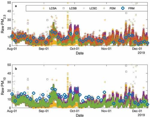
Figure 1 shows the time series of raw measurements from all sensors used in this study during the entire sample period, including the FRM and FEM. For raw PM_2.5 (Figure 1a), the LCSs follow the general trends of the FRM and FEM for the sampling period. However, it appears that LCS A recorded lower values during the period from September to October and LCS C recorded consistently lower values from September to December (see also Figure S5). As discussed below, during these periods, LCS A and C experienced shifts in the measurements, requiring different bias adjustment factors to bring their measurements into agreement with LCS B. The PM₁₀ values are shown in Figure 1b and display trends similar to measurements of PM_2.5; however, it is apparent that the recorded raw measurements of concentration are consistently lower than their reference data counterparts. This result may suggest that the LCSs are reading smaller PM more accurately or that they might not be accounting for all particles as they approach PM₁₀ size.

Figure 1. Panel a is the raw PM_2.5 and Panel b is the raw PM₁₀ concentration (µg/m3) data from the sensors at the Parklane site in Columbia, SC from August to December 2019. Sensors include FRM, FEM, LCS A, LCS B, and LCS C. 68 negative values from the FEM, on the PM_2.5 plot were not included.

As mentioned above, the data collected from the LCS was filtered into three categories and averaged for 1-hour and 24-hour time intervals for analysis and comparison. Table S1 presents a summary of the effects of filtering and averaging on the mean (standard deviation) and minimum/maximum PM_2.5 concentrations for LCS A, B, and C, the FRM, and the FEM for the duration that each sensor was deployed. It shows that LCS A and C had high standard deviations before filtering, attributable to the exceptionally high recorded values that were removed by retaining only the central 99% of data. After trimmed filtering, the maximum value and standard deviation decrease significantly for both sensors. Table S2 shows the summary statistics for each sensor for the timeframe when all were deployed and operational.

Overall, LCS B showed the lowest variance for trimmed data while LCS A showed the lowest variance for strict data. While strict hourly and daily values have a lower coefficient of variance; the strict hourly and daily categories have significantly fewer measurements than the trimmed hourly and daily categories.

Sensor-to-sensor variability

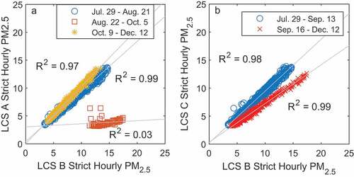
In addition to long-term sensor performance, this study assessed the sensor-to-sensor variability between the three LCSs. Figure 2 shows a pairwise comparison of strict hourly PM_2.5 data from LCS B contrasted with LCS A and LCS C. In both plots, there are distinct linear trends in the data, which have been distinguished in the figures by unique markers and individual trend lines. Inspection of Figure 2 shows that these trends correlate to specific time periods; three distinct time periods for A and two for C. It was observed that LCS A and C experience sudden changes in their measurements before shifting into a different operating regime. During these different periods, both LCS A and C maintain strong linear relationships to LCS B, but a different bias adjustment factor is needed to bring the measurements into closer agreement. Figure 2a shows three separate time periods for LCS A fit with determination coefficients: 0.97, 0.99 and 0.03. During the first period, July 29–Aug. 21, and third period, Oct. 9–Dec. 12, LCS A measurements were in line with LCS B. The time frame of Aug. 22–Oct. 5, LCS A records values noticeably lower than LCS B, with a RMSE of 10.6, and MAE of 10.4, and a correlation of 0.03 for the timeframe. For LCS C, Figure 2b shows two separate time periods fit with high coefficients of determination: 0.98 and 0.99. Similarly, contrasting LCS C with LCS B, the first time period, from Jul. 29 to Sep. 13, LCS C is in line with B, reporting a RMSE of 0.64, MAE of 0.52, and a correlation equal to 0.98 after which, from Sep. 14 to Dec. 12, LCS C begins consistently reporting lower values, reporting a RMSE of 2.3, MAE of 2.1, and a correlation equal to 0.99. Although two of the sensors had different modes, each shift remained linear, meaning the data can be adjusted for bias and corrected. To adjust for bias in LCS A and C, a simple linear regression to LCS B was done on the second- and third-time frame, Aug. 22–Oct. 5 and Oct. 9–Dec. 12, of LCS A and on the second time frame, Sep. 14–Dec. 12, of LCS C. The resulting fits were used to correct the data in those periods for LCS A and LCS C. Outside of these time periods, and for the entire sampling period for LCS B, no adjustment or correction to the data have been applied.

Figure 2. A pairwise comparison plot of the strict hourly PM_2.5 concentration measurements from the LCSs. Panel a shows the comparison of LCS A and B with three distinct trendlines indicting different date ranges; the yellow asterisks represent Jul.29 to Aug. 21, the orange squares indicate Aug. 22 – Oct. 5, and the blue circles indicate the time period from Oct. 9 – Dec. 12. Panel b shows a pairwise comparison of LCS B and C; the blue circles indicate the time frame from Jul. 29 to Sep. 13 and the red crosses indicate Sep. 16 – Dec. 12.

Low-cost sensor agreement to FEM

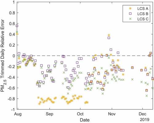
As mentioned above, the LCSs were compared to the FEM due to the lack of enough data for a robust analysis with the FRM. To show the performance of the FEM and its utility as a proxy for comparison, a plot contrasting the FEM to the FRM is included in Figure S6. The mean relative error of LCS measurements compared to the FEM was the lowest for all sensors immediately after initial deployment, from July 29 to August 21, after which point the mean relative error fluctuates for the LCSs. LCS B has the most consistent mean relative error for each time frame when compared to both LCS A and C, summarized in Table 3. LCS A has the highest relative error between Aug. 22 and Oct. 5, a mean relative error of −0.75 while LCS B has a mean relative error of −0.06. LCS C has the highest mean relative error between Sep. 13 and Dec. 12, −0.36 while LCS B has a mean relative error of −0.13. Figure 3 shows the relative error for trimmed daily measurements during the sampling campaign; the relative error for hourly trimmed measurements can be seen in Figure S7. LCS A and C, due to their variable performance during the sampling period in both trimmed and strict filtered categories, were adjusted for bias using LCS B as the standard before comparison with the FEM.

Figure 3. Plot of the relative error of trimmed daily measurements of the low-cost sensors versus the FEM at the Parklane site in Columbia, SC. Includes 93 values for each sensor.

Due to the small number of points available for strict daily comparison (24 values), the trimmed daily measurements (93 values) were used. Figure 4 shows the comparison of the bias adjusted trimmed daily PM_2.5 measurements, Figure 4a shows 45 comparable days between the FEM and the FRM from July 29–December 11, 2019. Figure 4b, c, and d show 93 daily trimmed values for the LCSs to the FEM. LCS A had the highest standard deviation when compared with the other LCSs, as well as the lowest R² value. The R² values and the linear regression equations are summarized in Table 4. For reference, a comparison of trimmed hourly LCS measurements with the FEM are presented in Figure S8 and a comparison of strict hourly LCS measurements with the FEM are in Figure S9.

Table 4. Linear regression summary for trimmed daily bias adjusted sensor measurements versus FEM.

X-Axis	Sensor	R^2	Linear Regression
FEM daily PM2.5	LCS A daily PM2.5	0.73	y = 0.98x − 1.3
FEM daily PM2.5	LCS B daily PM2.5	0.75	y = 0.98x − 1.5
FEM daily PM2.5	LCS C daily PM2.5	0.77	y = 1.0x − 1.6

Figure 4. A four-panel plot of the FEM versus the daily measurements for the FRM and LCSs. Panel a is a plot of 45 measurements between the FEM vs the FRM. Panels b, c, and d are of the FEM versus LCS A, B, and C respectively, and plots 93 trimmed bias adjusted daily measurements. Horizontal error bars represent the accuracy of the FEM +/- 0.75% while the vertical error bars represent the standard deviation of the average hourly measurements for the LCSs. The linear fit line is solid black and the 1:1 line is dashed.

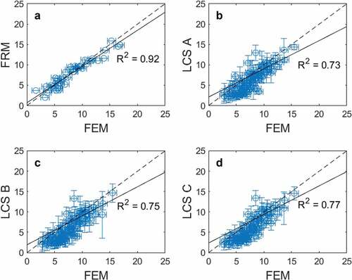
When comparing measurements, LCS B correlated the most with the FEM followed by LCS C and LCS A, respectively. After filtering and bias adjustment, however, LCS C correlated the most with the FEM, followed by LCS B and A. The poor correlation of LCS A appears to be largely attributable to a calibration shift that occurred in late August/early September and can be seen in Figure 3. Though the measurements from this time frame were adjusted for bias, the variability in the measurements during the bias adjusted time frame contributes to a lower coefficient of determination. In addition to the daily comparison, there are hourly comparisons for the FEM; 945 strict hourly measurements and 2300 trimmed hourly measurements. The strict and trimmed hourly measurements had R² values much smaller than the trimmed daily values, as expected for being averaged over a shorter duration of time, 1 hour compared to 24 hours.

Temperature and relative humidity dependence

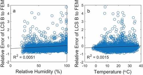
The correlation of the measurements of LCS B to relative humidity and temperature are 0.23 and 0.19, respectively. To better assess whether environmental conditions such as RH and temperature had an impact on the performance of the sensor, the relative error of the LCS measurements to the FEM were plotted as a function of RH and temperature. Figure 5 shows the relative error of trimmed hourly measurements from LCS B to the FEM compared to RH and temperature, both of which confirm the small impact of these variables on LCS B measurements; the R² values are 0.0051 and 0.0015 for trimmed hourly measurements, respectively. The relative error of trimmed hourly measurements from LCS A and LCS C to the FEM can be seen in Figures S10 and S11, respectively. Filtering out high values for RH and temperature both result in increases in dependence of the measurements on environmental factors; this is consistent with previous findings of inconsistent behavior of LCS in extreme environmental conditions. When filtering out measurements with associated RH values greater than 90%, the R² value is 0.007. Filtering out measurements with associated temperatures greater than 30 °C gives an R² value of 0.0017.

Figure 5. The ratio of hourly trimmed measurements of LCS B to the FEM plotted versus Relative Humidity (%) and Temperature (°C). This figure includes 2764 measurements, more than the 2300 measurements evaluated otherwise as these are only the measurements that are from LCS B compared to the FEM.

Conclusion

The Intelligent Air^TM sensor pack was evaluated from July 29, 2019 to December 12, 2019. The Sensirion SPS30 PM sensor tested in this study shows a potential for reliable long-term air quality measurements. At least one of the sensors, LCS B, showed good performance and linearity with the FEM throughout the duration of the study without the need for additional adjustment, while the other two sensors, LCS A and C, show linearity with the FEM after bias adjustment, indicating that corrective calibration is possible. Because the sensor packs were not evaluated in real-time during this study, it is not yet known the exact cause of the shifting calibrations; possible explanations include a failure in the self-cleaning feature, allowing debris to be temporarily lodged in the sensor housing, and extreme weather events. In future studies, changes in LCS performance can be evaluated by monitoring the relative error of the sensors to each other and/or to federal methods. Sharp increases or decreases in relative error can indicate a change in the sensor performance, something that artificial intelligence and machine learning models could identify in real-time. The LCS showed a low dependence on relative humidity when RH is less than 90%; however, further tests conducted in environments with RH>90% should be performed to ensure good performance in high RH conditions.

The versatile battery/solar power combination has kept the devices running for five months and two of them running for over a year. The data was easily accessed and downloaded in a comma separated value format from Grafana, an online interface, for analysis and the platform provides the ability to add new sensors and weather measurements. The main concern that needs investigation is the fluctuating bias of LCS A and LCS C. Further research is needed to understand the different offsets and measurement “modes” as well as the reason for shifting. However, because all the LCSs show linearity with FEM measurements, there is the potential for reliable long-term air quality measurements from the Sensirion SPS30. Additionally, as mentioned above, while LCSs are typically found to have poor coefficients of determination (R² < 0.1) when the ambient PM concentrations are below 20 µg m⁻³, the SPS30 in this study had a 1-hr R² of 0.34 for bias adjusted strict, 0.57 for bias adjusted trimmed, and a 24-hr R² of 0.75 for bias adjusted trimmed measurements in an environment that rarely exceeded 20 µg m⁻³. Recall also that LCS B did not have any bias adjustment factors applied to its measurements; the bias adjustment simply corrected clear shifts in sensor operating modes in the other two sensors deployed. Therefore, we think that the Intelligent Air^TM platform has the potential, with further testing, to become a highly deployable air quality monitoring station. Further testing with real-time monitoring will allow for in situ calibration adjustments to be determined, improving its’ potential for long term monitoring and remote deployment. Additionally, as LCSs do not typically have troubleshooting indicators, writing programs to monitor for non-ideal conditions for sensors has the potential to help identify when sensors are having issues, thus allowing for better analysis of the variables that contribute to poor sensor performance. Future research will include the evaluation and validation of the size speciation capabilities of the Sensirion SPS30 and the impacts of fluctuating weather conditions throughout the year, as this information may further refine the use cases for the sensor pack.

Acknowledgment

The authors would like to thank Kevin Watts, Scott Reynolds, and the staff at the Bureau of Environmental Health Services at the South Carolina Department of Health and Environmental Control for their assistance with deploying our sensors at the Parklane site and retrieving FEM/FRM particulate matter data. We also thank Sonoma Technologies for help obtaining large datasets of weather for the study period. The authors also would like to thank the SC Space Grant Consortium for their support of this work.

Disclosure statement

No potential conflict of interest was reported by the author(s).

Data availability statement

The data that support the findings of this study are available from the corresponding author, ARM, upon reasonable request.

Supplementary material

Supplemental data for this article can be accessed online at https://doi.org/10.1080/10962247.2022.2093293.

Additional information

Funding

This work was supported by SC NASA EPSCoR Research Infrastructure Development grant #NNX15AK53A; South Carolina Space Grant Consortium Graduate Research Fellowship #521383-GRF-CM005.

Notes on contributors

F.A. Roberts

F.A. Roberts is a master's student in Environmental Engineering at Clemson University whose research currently focuses on evaluating the use of low-cost sensors for air quality measurements in comparison with other methods.

Kathryn Van Valkinburgh

Kathryn Van Valkinburgh currently works as a licensed, professional engineer for an environmental consulting company. Her work focuses on air quality, permitting, and pollution control. She received her bachelor's and master's degrees in Environmental Engineering from Clemson University, where her research focused on air quality and the use of low-cost particulate matter sensing technology.

Austin Green

Austin Green holds an M.S. degree in Forest Resources from Clemson University. He is currently a senior land agent at Contract Land Staff (CLS) in Charlotte, NC, USA.

Christopher J. Post

Christopher J. Post holds a Ph.D. degree in Environmental Information Science from Cornell University. He is a professor of environmental information science in the Department of Forestry and Environmental Conservation at Clemson University, SC, USA.

Elena A. Mikhailova

Elena A. Mikhailova holds a Ph.D. degree in Soil Science from Cornell University. She is a professor of soil science in the Department of Forestry and Environmental Conservation at Clemson University, SC, USA.

Sarah Commodore

Sarah Commodore is a faculty member in the Department of Environmental and Occupational Health at the School of Public Health in Indiana University. Her research focus is on air pollution exposure assessment and toxicology.

John L. Pearce

John L. Pearce is an Associate Professor of Environmental Health and the leader of the Air Quality Lab at the Medical University of South Carolina. Dr. Pearce has expertise in exposure monitoring, modeling, and characterization and his research goal is to pioneer methodologies that will lead to breakthroughs in the understanding of links between complex environmental exposure and human health.

Andrew R. Metcalf

Andrew R. Metcalf is an Assistant Professor in Environmental Engineering and Earth Sciences at Clemson University. Dr. Metcalf leads the Clemson Air Quality Lab, where we have active projects to study air quality using low-cost sensors, particulate matter focusing on black carbon aerosol, and developing new measurement techniques using microfluidics.

References

- Astudillo, G. D., L. E. Garza-Castanon, and L. I. M. Avila. 2020. Design and evaluation of a reliable low-cost atmospheric pollution station in urban environment. IEEE Access. 8:51129–44. doi:10.1109/access.2020.2980736.
- Báthory, C., M. L. Kiss, A. Trohák, Z. Dobó, and Á. B. Palotás. 2019. Preliminary research for low-cost particulate matter sensor network. E3S Web Conf. 100:00004. doi:10.1051/e3sconf/201910000004.
- Bauerová, P., A. Šindelářová, Š. Rychlík, Z. Novák, and J. Keder. 2020. Low-cost air quality sensors: One-year field comparative measurement of different gas sensors and particle counters with reference monitors at Tušimice observatory. Atmosphere 11 (5):492. doi:10.3390/atmos11050492.
- Cavaliere, A., F. Carotenuto, F. D. Gennaro, B. Gioli, G. Gualtieri, F. Martelli, A. Matese, P. Toscano, C. Vagnoli, and A. Zaldei. 2018. Development of low-cost air quality stations for next generation monitoring networks: Calibration and validation of PM2.5 and PM10 sensors. Sensors 18 (9):2843. doi:10.3390/s18092843.
- Cho, E.-M., H. J. Jeon, D. K. Yoon, S. H. Park, H. J. Hong, K. Y. Choi, H. W. Cho, H. C. Cheon, and C. M. Lee. 2019. Reliability of low-cost, sensor-based fine dust measurement devices for monitoring atmospheric particulate matter concentrations. Int. J. Environ. Res. Public Health 16 (8):1430. doi:10.3390/ijerph16081430.
- Clements, A. L., S. Reece, T. Conner, and R. Williams. 2019. Observed data quality concerns involving low-cost air sensors. Atmos. Environ. X 3:100034. doi:10.1016/j.aeaoa.2019.100034.
- Commodore, S., A. Metcalf, C. Post, K. Watts, S. Reynolds, and J. Pearce. 2020. A statistical calibration framework for improving non-reference method particulate matter reporting: A focus on community air monitoring settings. Atmosphere 11 (8):807. doi:10.3390/atmos11080807.
- Demanega, I., I. Mujan, B. C. Singer, A. S. Anđelković, F. Babich, and D. Licina. 2021. Performance assessment of low-cost environmental monitors and single sensors under variable indoor air quality and thermal conditions. Build. Environ. 187:107415. doi:10.1016/j.buildenv.2020.107415.
- Feenstra, B., V. Papapostolou, S. Hasheminassab, H. Zhang, B. D. Boghossian, D. Cocker, and A. Polidori. 2019. Performance evaluation of twelve low-cost PM2.5 sensors at an ambient air monitoring site. Atmos. Environ. 216:116946. doi:10.1016/j.atmosenv.2019.116946.
- Gao, M., J. Cao, and E. Seto. 2015. A distributed network of low-cost continuous reading sensors to measure spatiotemporal variations of PM2.5 in Xi’an, China. Environ. Pollut. 199:56–65. doi:10.1016/j.envpol.2015.01.013.
- Jayaratne, R., X. Liu, K.-H. Ahn, A. Asumadu-Sakyi, G. Fisher, J. Gao, A. Mabon, M. Mazaheri, B. Mullins, M. Nyaku, et al. 2020. Low-cost PM2.5 sensors: An assessment of their suitability for various applications. Aerosol Air Qual. Res. doi:10.4209/aaqr.2018.10.0390.
- Jiang, H., H. Xiao, H. Song, J. Liu, T. Wang, H. Cheng, and Z. Wang. 2020. A long-lasting winter haze episode in Xiangyang, central China: Pollution characteristics, chemical composition, and health risk assessment. Aerosol Air Qual. Res. 20 (12):2859–73. doi:10.4209/aaqr.2020.02.0068.
- Jiao, W., G. Hagler, R. Williams, R. Sharpe, R. Brown, D. Garver, R. Judge, M. Caudill, J. Rickard, M. Davis, et al. 2016. Community Air Sensor Network (CAIRSENSE) project: Evaluation of low-cost sensor performance in a suburban environment in the southeastern United States. Atmos. Meas. Tech. 9 (11):5281–92. doi:10.5194/amt-9-5281-2016.
- Karagulian, F., M. Barbiere, A. Kotsev, L. Spinelle, M. Gerboles, F. Lagler, N. Redon, S. Crunaire, and A. Borowiak. 2019. Review of the performance of low-cost sensors for air quality monitoring. Atmosphere 10 (9):506. doi:10.3390/atmos10090506.
- Kelly, K. E., J. Whitaker, A. Petty, C. Widmer, A. Dybwad, D. Sleeth, R. Martin, and A. Butterfield. 2017. Ambient and laboratory evaluation of a low-cost particulate matter sensor. Environ. Pollut. 221:491–500. doi:10.1016/j.envpol.2016.12.039.
- Kuula, J., T. Mäkelä, M. Aurela, K. Teinilä, S. Varjonen, Ó. González, and H. Timonen. 2020. Laboratory evaluation of particle-size selectivity of optical low-cost particulate matter sensors. Atmos. Meas. Tech. 13 (5):2413–23. doi:10.5194/amt-13-2413-2020.
- Lehmann, K., A. Minhans, M. K. Fajari, and M. Hahn. 2019. Assessment of low-cost particulate matter sensors. ISPRS Int. Arch. Remote Sens. Spatial Inf. Sci. XLII-4/W18:671–77. doi:10.5194/isprs-archives-xlii-4-w18-671-2019.
- Li, J., S. K. Mattewal, S. Patel, and P. Biswas. 2020. Evaluation of nine low-cost-sensor-based particulate matter monitors. Aerosol Air Qual. Res. 20 (2):254–70. doi:10.4209/aaqr.2018.12.0485.
- Lim, C.-H., J. Ryu, Y. Choi, S. W. Jeon, and W.-K. Lee. 2020. Understanding global PM2.5 concentrations and their drivers in recent decades (1998–2016). Environ. Int. 144:106011. doi:10.1016/j.envint.2020.106011.
- Liu, J. C., A. Wilson, L. J. Mickley, F. Dominici, K. Ebisu, Y. Wang, M. P. Sulprizio, R. D. Peng, X. Yue, J.-Y. Son, et al. 2017. Wildfire-specific fine particulate matter and risk of hospital admissions in urban and rural counties. Epidemiology 28 (1):77–85. doi:10.1097/ede.0000000000000556.
- Liu, X., R. Jayaratne, P. Thai, T. Kuhn, I. Zing, B. Christensen, R. Lamont, M. Dunbabin, S. Zhu, J. Gao, et al. 2020. Low-cost sensors as an alternative for long-term air quality monitoring. Environ. Res. 185:109438. doi:10.1016/j.envres.2020.109438.
- Motlagh, N. H., M. A. Zaidan, P. L. Fung, E. Lagerspetz, K. Aula, S. Varjonen, M. Siekkinen, A. Rebeiro-Hargrave, T. Petäjä, Y. Matsumi, et al. 2021. Transit pollution exposure monitoring using low-cost wearable sensors. Transp. Res. Part D 98:102981. doi:10.1016/j.trd.2021.102981.
- Mukherjee, A., L. Stanton, A. Graham, and P. Roberts. 2017. Assessing the utility of low-cost particulate matter sensors over a 12-week period in the Cuyama Valley of California. Sensors 17 (8):1805. doi:10.3390/s17081805.
- Post, C. J., M. P. Cope, P. D. Gerard, N. M. Masto, J. R. Vine, R. Y. Stiglitz, J. O. Hallstrom, J. C. Newman, and E. A. Mikhailova. 2018. Monitoring spatial and temporal variation of dissolved oxygen and water temperature in the Savannah River using a sensor network. Environ. Monit. Assess. 190 (5):272. doi:10.1007/s10661-018-6646-y.
- Post, C. J., E. A. Mikhailova, J. L. Sharp, A. H. Nelson, M. P. Cope, J. O. Hallstrom, and R. D. Chandler. 2019. Detecting river-scale turbidity disturbance after rainfall using NEXt-Generation Weather RADar (NEXRAD) and the Intelligent River. J. Soil Water Conserv. 74 (2):101–10. doi:10.2489/jswc.74.2.101.
- Qin, X., L. Hou, J. Gao, and S. Si. 2020. The evaluation and optimization of calibration methods for low-cost particulate matter sensors: Inter-comparison between fixed and mobile methods. Sci. Total Environ. 715:136791. doi:10.1016/j.scitotenv.2020.136791.
- SC DHEC. 2020. State of South Carolina, annual ambient air monitoring network plan, July 1, 2020 - December 31, 2021. Bureau of Air Quality, South Carolina Department of Health & Environmental Control.
- US EPA. 2006. Electronic code of federal regulations (eCFR).
- US EPA. 2009. Quality assurance project plan for the federal PM2.5 performance evaluation program.
- US EPA. 2020. Air quality system data mart air quality statistics report. Accessed June 18, 2020. https://www.epa.gov/airdata
- Zamora, M. L., F. Xiong, D. Gentner, B. Kerkez, J. Kohrman-Glaser, and K. Koehler. 2018. Field and laboratory evaluations of the low-cost plantower particulate matter sensor. Environ. Sci. Technol. 53 (2):838–49. doi:10.1021/acs.est.8b05174.
- Zheng, T., M. H. Bergin, K. K. Johnson, S. N. Tripathi, S. Shirodkar, M. S. Landis, R. Sutaria, and D. E. Carlson. 2018. Field evaluation of low-cost particulate matter sensors in high- and low-concentration environments. Atmos. Meas. Tech. 11 (8):4823–46. doi:10.5194/amt-11-4823-2018.