Assessment of light-duty versus heavy-duty diesel on-road mobile source emissions using general additive models applied to traffic volume and air quality data and COVID-19 responses

ABSTRACT

Following the outbreak of the COVID-19 pandemic, several papers have examined the effect of the pandemic response on urban air pollution worldwide. This study uses observed traffic volume and near-road air pollution data for black carbon (BC), oxides of nitrogen (NO_x), and carbon monoxide (CO) to estimate the emissions contributions of light-duty and heavy-duty diesel vehicles in five cities in the continental United States. Analysis of mobile source impacts in the near-road environment has several health and environmental justice implications. Data from the initial COVID-19 response period, defined as March to May in 2020, were used with data from the same period over the previous two years to develop general additive models (GAMs) to quantify the emissions impact of each vehicle class. The model estimated that light-duty traffic contributes 4–69%, 14–65%, and 21–97% of BC, NO_x, and CO near-road levels, respectively. Heavy-duty diesel traffic contributes an estimated 26–46%, 17–63%, and −7–18% of near-road levels of the three pollutants. The estimated mobile source impacts were used to calculate NO_x to CO and BC to NO_x emission ratios, which were between 0.21–0.32 μg m⁻³ NO_x (μg m⁻³ CO)⁻¹ and 0.013–0.018 μg m⁻³ BC (μg m⁻³ NO_x)⁻¹. These ratios can be used to assess existing emission inventories for use in determining air pollution standards. These results agree moderately well with recent National Emissions Inventory estimates and other empirically-derived estimates, showing similar trends among the pollutants. However, a limitation of this study was the recurring presence of an implausible air pollution impact estimate in 41% of the site-pollutant combinations, where a vehicle class was estimated to account for either a negative impact or an impact higher than the total estimated pollutant concentration. The variations seen in the GAM estimates are likely a result of location-specific factors, including fleet composition, external pollution sources, and traffic volumes.

Implications: Drastic reductions in traffic and air pollution during the lockdowns of the COVID-19 pandemic present a unique opportunity to assess vehicle emissions. A General Additive Modeling approach is developed to relate traffic levels, observed air pollution, and meteorology to identify the amount vehicle types contribute to near-road levels of traffic-related air pollutants (TRAPs), which is important for future emission regulation and policy, given the significant health and environmental justice implications of vehicle-related pollution along major roadways. The model is used to evaluate emission inventories in the near-road environment, which can be used to refine existing estimates. By developing a locally data-driven method to readily characterize impacts and distinguish between heavy and light duty vehicle effects, local regulations can be used to target policies in major cities around the country, thus addressing local health disbenefits and disparities occurring as a result of exposure to near-road air pollution.

Introduction

The first documented case of COVID-19 in the United States was recorded on January 20, 2020 in Washington State. A little over a month later, on March 3, Washington State declared a state of emergency, later issuing a 10-week stay-at-home order (SHO) lasting from March 23 through the end of May 2020 (Mitchell et al. 2020). As the virus continued to spread, states around the country followed suit, enacting stay-at-home orders to varying degrees (Lasry et al. 2020; Wu et al. 2020). As a result of these state-issued orders, traffic volume levels across the country decreased dramatically (Chen et al. 2021; Du et al. 2020; Highway Data Services Bureau 2021; Hudda et al. 2020; Xiang et al. 2020). In downtown Seattle, for example, traffic on Interstate-5 (I-5) was 50% lower in April than in February 2020 (Xiang et al. 2020). On urban expressways in New York City, monthly average daily traffic (MADT) decreased by 15–50% for the months of March through May 2020 (Highway Data Services Bureau 2021). A substantial amount of research has already been done to investigate the impact of this decrease in traffic volume on urban air pollution levels (Bar et al. 2021; Bauwens et al. 2020; Berman and Ebisu 2020; Elshorbany et al. 2021; Hudda et al. 2020; Tanzer-Gruener et al. 2020; Xiang et al. 2020). Previous studies in China, for example, have shown that ambient levels of particulate matter less than or equal to 2.5 microns in diameter (PM_2.5), nitrogen dioxide (NO₂), and carbon monoxide (CO) decreased by 30–40%, 30–60%, and 30%, respectively, during the COVID-19 period (Shi and Brasseur 2020; Xu et al. 2020). Studies in the Seattle area have shown smaller, though still significant, decreases for median black carbon (BC), oxides of nitrogen (NO_x), and CO levels across the same period. Using MAR(1) models to predict the air pollution impacts from current-hour road occupancy, one study estimated that COVID lockdowns caused a 6%, 6%, and 4% decrease in median levels of BC, NO_x, and CO, respectively, when comparing the four weeks prior to the SHO to the 10-week period immediately following the order (Xiang et al. 2020).

A study of several European and US cities found a −25% and −35% relative percentage deviation (RPD) of ground-based measurements of NO₂ in New York City and Boston, respectively, during the COVID-19 lockdowns (March 22 to May 30, 2020) when compared to the same period in 2019. The study also used TROPOMI satellite measurements to estimate changes in NO₂ concentration, which found an RPD of 26.6% in New York City and 18.6% in Boston between the two periods. The RPD for ground-based PM_2.5 measurements in both cities was −10% and −7.8%, respectively. TROPOMI and ground-based results were compared between cities that enacted strict lockdowns (i.e., New York City) and those that did not (i.e., Bismarck, ND), and lockdowns were found to lead to relative increases in the drop in air pollution levels, though cities without lockdowns still experienced significant decreases in air pollution (Bar et al. 2021).

Extended exposure to high concentrations of these air pollutants has been shown to cause adverse health effects in groups of all ages (Braga et al. 2001; Hoek et al. 2013). Communities living along major roadways, which tend to be low-income or minority populations (Park and Kwan 2020; Tian, Xue, and Barzyk 2012), experience increased and extended exposure to air pollution (Hajat, Hsia, and O’Neill 2015; Lal, Ramaswami, and Russell 2020), meaning the source classification of emissions in the near-road environment has significant health and environmental justice implications.

Here, the practicality of using the relationships between decreases in traffic and ambient air pollutant levels as a means of determining the contributions of light-duty (LD) and heavy-duty diesel (HD) traffic to near-road urban air pollution in the US is investigated. This method is also used to assess emission inventories of mobile sources. Specifically, this study uses COVID-19 restrictions in Seattle, Atlanta, New York City (Queens), Oakland, and the South Coast Air Basin (SoCAB) of California (which includes Los Angeles) to assess the contribution of HD and LD vehicles to ambient near-road pollution levels of BC, NO_x, and CO. General additive models (GAM) are developed to control for meteorological factors while quantifying the role of both vehicle classes.

Methods

General approach

General additive models were used to develop associations between traffic volumes and near-road air quality, accounting for meteorology (Aldrin and Haff 2005), using hourly near-road air quality monitoring data and traffic volumes at seven sites in five cities around the country. GAMs use smooth functions to fit functional relationships to the independent predictor variables. Here, cubic splines are used to fit the independent variables (traffic volumes, meteorological variables) to the observed air quality of CO, NO_x and BC. The GAMs used data from before and during the COVID-19 pandemic to capture any correlations between decreased traffic volumes and improved air quality during the period of initial and heightened COVID-19 response (Figures 1 and 2 and Table 1). Using meteorological factors in the GAM controls for meteorological variations between years.

Figure 1. Average daily traffic counts across all studied sites in the pre-COVID (March – May 2018 and 2019) and COVID (March – May 2020) periods.

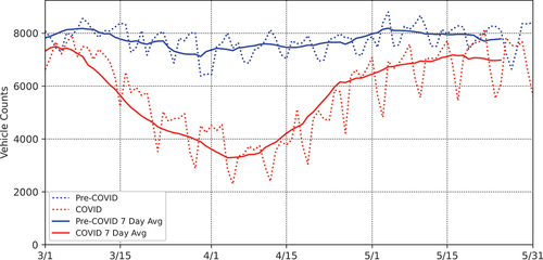
Figure 2. Average (a) BC, (b) NO_x, and (c) CO concentrations across all studied sites in the pre-COVID (March – May 2018 and 2019) and COVID (March – May 2020) periods.

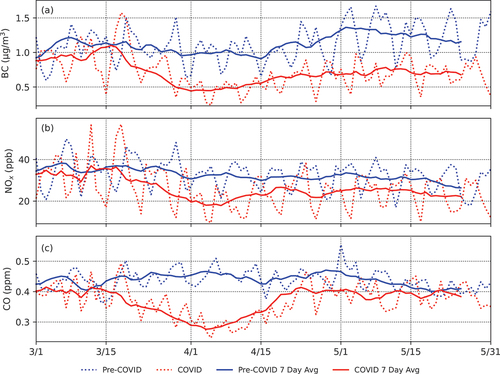
Table 1. Changes in average hourly pollutant concentration and average hourly traffic count at each site from pre-COVID period to COVID period.

Site	ΔBC (μg/m^3)	ΔNOx (ppb)	ΔCO (ppm)	ΔTraffic (vehicles)
Anaheim	–	−9.4	−0.22	−241
Atlanta	−0.62	−0.39	−0.02	−3421
Long Beach	–	−5.13	–	−3320
Oakland	−0.3	−9.7	−0.04	−2620
Ontario	–	−4.38	−0.02	−1755
Queens	−0.39	−7.34	−0.07	−1198
Seattle	−0.38	−12.68	−0.06	−2420

Model input data

Hourly air pollution, classed traffic, and meteorological data were collected for March 1 to May 31 in 2018, 2019, and 2020. Data from 2018 and 2019 were categorized as the “pre-COVID” period, while data from 2020 were categorized as the “COVID” period. The dates in 2020 align with the general period of the preliminary COVID-19 response when the greatest traffic reductions were generally experienced (Chen et al. 2021; Du et al. 2020; Highway Data Services Bureau 2021; Xiang et al. 2020). While the actual duration and timing of COVID-related policies did not always correspond perfectly with the “COVID” period (Wu et al. 2020), the public’s reaction (Czeisler et al. 2021), as well as corporate policy, to the pandemic during these dates still resulted in decreased traffic levels on major roadways during the periods analyzed (Bick, Blandin, and Mertens 2020; Lasry et al. 2020). Data from the pre-COVID period were selected from only two years to avoid biasing the model too far toward a typical year, while including multiple observations for each date and time.

This study used hourly near-road ambient air pollution data from the United States Environmental Protection Agency’s Near-Road (monitoring) Network (Ambient Monitoring Technology Information Center 2020; United States Environmental Protection Agency), which was started as part of the 2010 NO₂ National Ambient Air Quality Standards (NAAQS) review. The network consists of monitoring sites chosen for their high-traffic locations, where traffic-related air pollutants (TRAPs), specifically of NO₂, are expected to reach a maximum (Lal, Ramaswami, and Russell 2020). Though the sites are only required to measure NO₂, many sites also monitor other pollutants, including BC, NO_x, and CO, which were the focus of this investigation. NO_x is used instead of NO₂ as that is the mobile source emissions of concern, most of which occur as NO (Wild et al. 2017). Furthermore, the atmospheric NO₂ to NO_x ratio varies depending on meteorology and the presence of other pollutants (Mavroidis and Ilia 2012). Similarly, BC and elemental carbon (EC) are strongly correlated carbonaceous species and differ only in their measurement protocols, where BC is measured optically, and EC is measured thermally (Salako et al. 2012). BC was chosen for this study because it was more commonly measured at the selected sites. Seven near-road monitoring sites from five major urban areas, in different regions of the country, were selected for this study, including one site each in Seattle, Atlanta, New York (Queens), and Oakland (in the San Francisco, CA area) and three sites in the greater Los Angeles area. Each of these sites measured at least one of the three pollutants under investigation (Table 2). Use of near-road monitoring data allows focusing on the most immediate emissions as the transport times between the roadway and monitoring site is small.

Table 2. Traffic and air monitor site information. Sites highlighted in yellow are sites considered to be in the Los Angeles area (SoCAB). Each site is referred to by the respective city name instead of the EPA site name for brevity. “Travel feature” refers to any roadway, while “mainline” refers to a highway specifically (the target roadway). Certain site observations may be affected by the nearby “Travel feature” if it is a large enough road that is not the target roadway.

Hourly traffic data, by class, were obtained from each state’s respective Department of Transportation (California Department of Transportation; Georgia Department of Transportation; Highway Data Services Bureau; Washington State Department of Transportation). In most cases, data were obtained from a traffic monitor along the target roadway of the corresponding air monitor, except for Atlanta, Seattle and Queens (Table 2). At the Atlanta site, the target roadway is Interstate-85 (I-85). The closest traffic monitor to the air monitoring site is located on Interstate-75 (I-75) at the junction with I-85 (Georgia Department of Transportation). The Seattle site was located at the intersection of two major roadways: Interstate-5 (I-5), the target roadway, and Interstate- 90 (I-90). None of the I-5 traffic monitors within the vicinity of the near-road air monitor recorded classed traffic information (Washington State Department of Transportation 2019). As a result, data from the nearest traffic monitor along I-90 was used instead. In the case of the Queens site, no continuous traffic monitors were located along the air monitor’s target roadway, Interstate-495, nor any nearby intersecting roadways, though three traffic monitors were in the same neighborhood (Highway Data Services Bureau; New York State Department of Transportation). Lane-adjusted traffic data from these three sites were averaged to estimate the traffic at the monitoring site location. Despite the use of aggregate traffic counts, the Queens site was included in this investigation because of the significant drop in traffic levels reported by the New York State Department of Transportation during the COVID-19 lockdown (Highway Data Services Bureau 2021).

Classed traffic data obtained from each state’s Department of Transportation were typically recorded using the Federal Highway Administration’s (FHWA) existing 13-type classification system, which classifies traffic in a series of groups ranging from motorcycles as Group 1 to multi-trailer trucks as Group 13 (United States Federal Highway Administration 2014). For the purposes of this study, the FHWA system was simplified into only two classes based on typical engine and fuel type for that group: light-duty (LD) traffic, consisting of commuter vehicles (Groups 1–3), versus heavy-duty (HD) traffic, consisting of larger commercial vehicles (Groups 4–13).

Hourly meteorological data for this study, including hourly wind speed and temperature, were primarily obtained from the US National Oceanic and Atmospheric Administration’s (NOAA’s) National Centers for Environmental Information, using the U.S. Local Climatological Data (LCD) dataset (National Centers for Environmental Information, NESDIS, NOAA, and U.S. Department of Commerce). The one exception to this was the Seattle site, where meteorological data was obtain directly from the near-road air monitoring site itself (). After the initial analysis, wind speed was deemed the most significant and driving meteorological factor impacting ambient air pollution levels (Aldrin and Haff 2005), and thus was the only factor finally adopted for use in the GAM.

General additive model

This study developed general additive models (GAM) to assess the impact of each vehicle class on ambient pollution levels in each location. The GAM was constructed using the “mgcv” package in R, which is a “mixed GAM computation vehicle with automatic smoothness estimation” (2022; R: A Language and Environment for Statistical Computing 2021). The dependent variable in the model was the hourly concentration of the pollutant (y_t) at time t, while the independent predictor variables were the day of the year that the data was collected (d_t), the hour of the day (t_t), the LD traffic volume at that hour (LD_t), the HD traffic volume at that hour (HD_t), and the wind speed at that hour (wt). The GAM can be represented as:

(1) $y_t={\beta }_0+f_0(d_t)+f_1(t_t)+f_2(L{D}_t)+f_3(H{D}_t)+f_4(w_t)+\epsilon$(1)

where β₀ is a constant, f₀ – f₄ are nonparametric (smooth) functions estimated by the model, and ε is the residual. A single model was developed for weekdays and weekends together to take advantage of the traffic and air quality variations between those periods. Model outputs were the air pollutant concentrations for each hour of each day during the modeled periods.

Other versions of the model were initially considered, including a logarithmic transformation of the pollutant concentration, as is often done (Aldrin and Haff 2005), and the inclusion of other meteorological variables. Testing of each model was done by generating a diurnal plot showing the average concentration of each pollutant both as estimated by the model and as measured by the near-road monitor (Figure 3). R-squared and standard error values were considered, and a visual inspection was performed to determine how well each model’s averages matched the observed averages before the final selection was made.

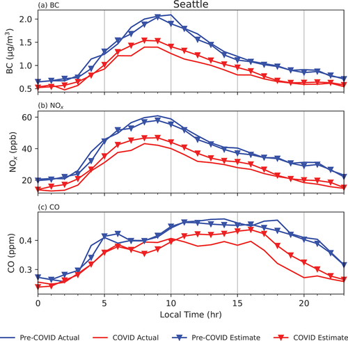
Figure 3. Time series of average GAM-predicted pollutant concentrations and average observed pollutant concentrations in the period before COVID-19 lockdowns (pre- COVID) and during the COVID-19 lockdowns (COVID) at the Seattle site. See SI Figure S5 for results from all sites.

The GAM for each site-pollutant pair was then used to estimate the average percent contribution of LD and HD vehicles to both mobile source impacts and total near-road impacts. Mobile source impacts were defined as the sum of the impacts from LD and HD vehicles, while total near-road impacts were defined as the wind-adjusted pollution levels as estimated by the model. Wind adjustment was done by estimating the pollution concentration at each point if the wind speed was zero, thus removing the impact of variations in wind speed from the rest of the analysis. Pollutant specific near-road air quality impact ratios were calculated from these mobile source impact estimates in two ways: 1) as the ratio between the total mobile source impacts of one pollutant to the total mobile source impacts of another pollutant; 2) as the slope of an orthogonal regression line relating the hourly mobile source impact estimates of the two pollutants (Lal, Ramaswami, and Russell 2020).

The GAM model, as specified, does not include any lag term (i.e., accounting for traffic volumes from previous hours), which is justified by using near-road monitors that are located within seconds to minutes of transport time from the highways, while the traffic, air quality and meteorology data are hourly. Additionally, the lag term is highly correlated with the current term, meaning that excluding this term avoids multicollinearity within the model (SI Table S4).

Separate weekend and weekday models were also considered, though they performed no better, so the main analysis uses the model including each day of the week as that approach utilizes weekday-weekend variations in specifying model terms.

While the hour of day and day of year variables help account for temporal background air quality variations, the model does not account for random background air quality variations (the intercept is constant). This is a model limitation, though near-road monitoring locations are chosen to be maximally impacted by the adjacent highway(s).

Model evaluation

Several model parameters were considered to evaluate the GAM for each site and pollutant. The primary statistics were the adjusted R² (referred to simply as R²) value of the model, which accounts for the number of predictor variables to determine if the addition of these variables increased the model fit. The R² value for each model was calculated directly using the “mgcv” package in R during the model construction (R: A Language and Environment for Statistical Computing 2021). This was used in the selection of the final predictor variables and in determining the relative strength of models across different sites and pollutants.

When evaluating the model, the root mean square error (RMSE) and normalized RMSE were also considered (Emery et al. 2017). RMSE calculates the standard deviation of the residuals in a model, which can indicate how well the data is concentrated around the model. Low RMSE values were used to indicate a higher accuracy of GAM estimates compared with their corresponding observed values. The RMSE was normalized with respect to the average observed pollution level. The normalized mean bias error (MBE) was also considered only to quantify the bias of the model and determine which parameters (if any) were helping to correct this bias. These statistics were calculated for both the pre-COVID and COVID periods independently to assess the strength of the model in each individual period. A daily (instead of hourly) statistic was also calculated using the aggregate of estimates and observations across each day of the study with at least 21 hours of observations.

After considering these different evaluation statistics, a visual inspection was also performed on the model by creating a diurnal plot overlaying the average hourly GAM estimates and the average hourly observed pollution levels at each site in each period. This inspection was performed to determine the general success of the model throughout the day. It also helped determine which predictor variables helped or did not help account for daily fluctuations.

Results

Hourly near-road pollution estimates

GAM results show varying levels of agreement between the observed and predicted BC, NO_x, and CO near-road concentrations, depending on location and pollutant (Figure 4). Model-estimated percent contributions of both LD and HD traffic to mobile source impacts and total near-road air pollution in both the pre-COVID and COVID periods also show varying results depending on location (Figures 5–7).

Figure 4. Average hourly percent bias of GAM-estimated concentrations to observed concentrations for each pollutant at the Seattle site over the pre-COVID and COVID periods. See SI Figure S6 for results from all sites.

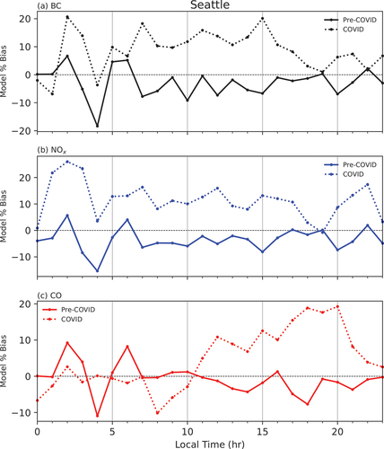
Figure 5. BC emission contributions of LD traffic, HD traffic, and mobile sources combined as a percentage of wind-adjusted near-road levels as estimated by the GAM during the pre-COVID period. An asterisk (*) denotes a site-pollutant combination in which the average estimated contribution of at least one vehicle class (LD, HD, or combined) in any period (note that only pre-COVID is shown) is either negative or greater than the wind-adjusted average estimate for at least one hour during the day. See SI Figure S7 for contributions during the COVID period.

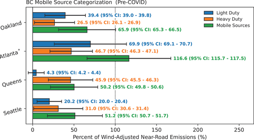
Figure 6. The same as Figure 5 but for NO_x emissions. Note that the Ontario and Atlanta sites are marked with an asterisk (*) but do not seem to show signs of any implausibility in this figure. The implausibility occurs at an hour during the day. See SI Figure S7 for contributions during the COVID period.

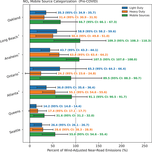
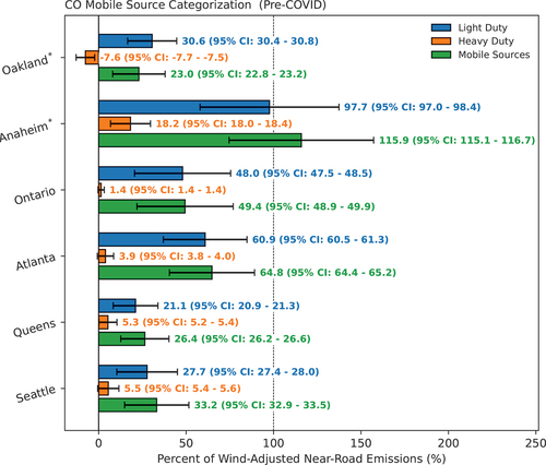
Figure 7. The same as Figure 5 but for CO emissions. See SI Figure S7 for contributions during the COVID period.

In all cases, the GAM captured decreases in air pollutant concentrations between the pre-COVID and COVID periods (Table 1). On an hourly basis, R²s ranged from 0.17 to 0.51, indicating a site- and pollutant-specific variation.

In Seattle, which was one of the first US cities to enter a state of emergency in response to the COVID-19 pandemic (Lasry et al. 2020; Wu et al. 2020), the GAM-predicted hourly average impacts visually align closely with the observed hourly average impacts, suggesting that the GAM captures the traffic-air quality relationship well (Figures 3 and 4). The coefficients of determination (R² values) for the models for each pollutant are between 0.34 and 0.37. The normalized root mean square error (NRMSE) for the three pollutants is between 0.27 and 0.69, with the lowest NRMSE in the CO model and the highest in the BC model (Table 3).

Table 3. Model results and error metrics for each site-pollutant combination on an hourly basis. Blue rows represent metrics from the pre-COVID period, while orange rows represent metrics from only the COVID period. The average in parentheses represents the observed average concentration, while the average outside of parentheses represents the average concentration as estimated by the GAM.

At the Queens site, a side-by-side visual inspection of the model-estimated hourly averages and observed hourly averages suggests that the GAM can capture the differences between the pre-COVID and COVID periods, though the estimated effects of the COVID pandemic are not as pronounced as in the observed averages. For BC especially, the model is consistently overestimating COVID pollution levels, with an hourly percent error of>25% throughout the day (Figure 4). This overestimation, evident at all sites, likely occurs because a single model was built using the data across both periods, operating on the assumption that observed air pollution differences between the two periods occurred solely because of different traffic levels. The R² values for each pollutant are between 0.29 and 0.37, with the lowest R² value from the CO model. The NRMSE values are between 0.31 and 0.97, with the lowest NRMSE occurring in the CO model and the highest in the BC model (Table 3).

In Atlanta, even though the observed concentrations of the three pollutants did not drop as significantly during the COVID period, the average GAM estimates still visually matched the observed averages to a high degree (Figure 4). The R² values at the Atlanta site were between 0.3 and 0.49, the latter, which was for NO_x, being the second highest R² of all cases. Likewise, the NRMSE values also tended to be lower at the Atlanta site, between 0.29 and 0.54 (Table 3). The combination of a high R² and low NRMSE suggests that the Atlanta models provide a strong estimate of the data. The Oakland site also performs well under a visible inspection (Figure 4) and has R² values between 0.33 and 0.51 across the three pollutants, indicating that the model captures the data variation well. The NRMSE across the three pollutants ranges from 0.2 for CO to 0.67 for BC (Table 3). These four sites generally show a good fit of the model, especially for CO, which had the lowest NRMSE of the three pollutants at each site.

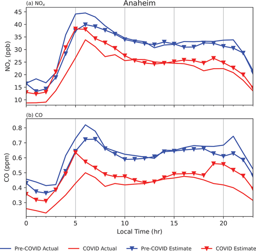
Application of the method to sites in California’s SoCAB, namely Anaheim, Long Beach, and Ontario, find that the average estimated hourly impacts do not visually align as well to the average observed hourly impacts as in other sites. In these three cases, the model consistently does not capture the large morning peak of observed concentrations around 6-7am during the pre-COVID period (Figures 4 and 8). This observation could indicate that non-freeway traffic (which is not accounted for in this study) impacts near-road emissions monitors in this area more than is suggested by increases in the freeway traffic data. Alternatively, it could be an indication that the contributions of different vehicles are more nuanced than the two-class simplification used in this model or that other meteorological factors warrant inclusion in the model in the SoCAB specifically. The R² value for the model in each SoCAB site-pollutant combination is between 0.17 and 0.47, while the NRMSE ranges from 0.28 to 0.92. The Long Beach NO_x model has one of the lowest R² values, 0.2, and the highest NRMSE, 0.92, meaning it is not a strong fit of the observed data (Table 3).

Figure 8. Time series of average GAM-predicted pollutant concentrations and average observed pollutant concentrations in the period before COVID-19 lockdowns (pre- COVID) and during the COVID-19 lockdowns (COVID) at the Anaheim site. See SI Figure S5 for results from all sites.

Effect of day of week on model error

In general, weekday estimates (Mon-Fri) of LD and HD impacts align better than weekend (Sat & Sun) estimates with their observed counterparts, especially when considering NO_x and CO, though the former is most pronounced (Figure 9). This could be explained by more standardized traffic patterns during weekday commuting (Agarwal 2004), leading to consistent peaks in both traffic and observed near-road pollution levels (Morawska et al. 2002), and that HD vehicles account for much of the NO_x impacts. Additionally, each model was also developed using data across the entire week, which skews the hour-of-day predictor variable to follow weekday trends because of the greater frequency of weekday samples. The BC model does not follow this behavior, however, and instead shows an increase in model bias in the mid-to-late week (Thu-Sat), meaning the BC model disagreement is likely the result of another external factor, not traffic patterns (Figure 9).

Figure 9. Average percent bias of the model across all sites for each day of the week for each pollutant: (a) BC, (b) NO_x, (c) CO.

Mobile source contributions

When using the GAM to estimate contributions of LD and HD traffic to near-road air pollution levels, similarities are observed for each pollutant across multiple sites. The specific estimated contributions are city-dependent as they are likely affected by external emission sources (Mueller et al. 2011; United States Environmental Protection Agency 2017), road occupancy, fleet composition, and other location-specific factors (Boriboonsomsin and Barth 2008; Cicero-Fernândez, Long, and Winer 1997; Tang et al. 2019; Wyatt, Li, and Tate 2014), but several general ideas can be seen at multiple locations. These results focus on pre-COVID estimates as they are representative of a typical year and are therefore of greater interest. We use the GAM model estimates of category-specific impacts on near-road air quality as estimates of relative emissions impacts.

In the case of CO emissions impact on air quality, LD traffic was found to be the primary contributor, comprising an estimated 60.9% (95% CI: 60.5–61.3%), 48.0% (95% CI: 47.5–48.5%), 21.1% (95% CI: 20.9–21.3%), and 27.7% (95% CI: 27.4–28.0%) of the total observed CO in Atlanta, Ontario, Queens, and Seattle, respectively, in pre-COVID times. In comparison, the largest estimated contribution of HD traffic to CO was 5.5% (95% CI: 5.4–5.6%), in Seattle (Figure 7), which is not surprising given that diesel engines are lower emitters of CO than gasoline engines. These estimates show moderate agreement with established county-level National Emissions Inventories (NEI), the most granular regional estimates released every three years by the EPA. In 2017, the year of the latest release, LD traffic was estimated to contribute 59% and 44% of all CO emissions in San Bernardino and Fulton counties, which are the respective counties for the Ontario and Atlanta sites (United States Environmental Protection Agency 2017). The NEI emissions are both within 4% of the contributions estimated by the GAM. The NEI estimates are from 2017 and their accuracy has recently been debated (Lal, Ramaswami, and Russell 2020; McDonald et al. 2018; Qin et al. 2019), but they still provide a benchmark of comparison for the GAM estimates from 2018 and 2019. In Queens, NY, and King, WA, counties, corresponding to the Queens and Seattle sites, the NEI estimates suggest that LD traffic contributes 42% and 43% of CO emissions respectively (United States Environmental Protection Agency 2017), nearly double both GAM estimates. It should be noted that the NEI emissions are county-wide emissions, not specifically near-road emissions, meaning that greater weight is likely given to mobile sources in the GAM estimates, and the disagreement between the NEI and GAM results would increase if the NEI estimates were specific to the near-road environment. In addition, CO has a background level of about 0.17–0.44 ppm, which is also a factor in how mobile source emissions impact CO levels. When considering HD traffic, the NEI estimate that HD traffic contributes 3–4% of CO emissions in each of the four counties (United States Environmental Protection Agency 2017), which agrees well with the GAM results. Despite disagreement of specific contributions, the GAM results agree with the NEI trend, in which LD traffic dominates mobile source emissions of CO.

NO_x contribution results were not nearly as dominated by one vehicle class, with the GAM estimating that both LD and HD traffic contributed roughly equal levels of near-road NO_x emissions at several sites. In Oakland, Queens, and Seattle, LD traffic contributed 35.8% (95% CI: 34.9–35.7%), 14.2% (95% CI: 14.0–14.4%), and 26.4% (95% CI: 26.1–26.7%) of near-road emissions, while HD traffic contributed a similar 31.4% (95% CI: 30.9–31.9%), 17.4% (95% CI: 17.1–17.7%), and 28.6% (95% CI: 28.3–28.9%) of near-road emissions, respectively. Mobile sources combined contributed to an estimated 66.7% (95% CI: 66.1–67.3%), 31.6% (95% CI: 31.2–32.0%), and 55.0% (95% CI: 54.6–55.4%) of total near-road NO_x levels in those cities (Figure 6). The NEI estimates that 46%, 28%, and 48% of NO_x emissions in Alameda (which corresponds to the Oakland site), Queens, and King counties come from mobile sources (United States Environmental Protection Agency 2017), which show variable agreement with the GAM results in the corresponding cities. The GAM results are higher, which is not surprising, given the roadway proximity.

Despite the absolute 20% disagreement between GAM and NEI results at the Oakland site, a similar study using machine-learning models applied to the COVID-period showed that HD traffic reductions accounted for 61% of traffic-induces changes in NO₂ in the LA area (Yang et al. 2021), which shows strong agreement with the GAM. At the Queens and Seattle sites, NEI results differed by only an absolute 3.6% and 7%. However, the results for Seattle did not agree as strongly when considering the breakdown of these mobile source emissions. Using NEI estimates, LD traffic was estimated to account for 68% of mobile source NO_x emissions in King County, a contribution almost 1.5 times greater than the 48% (95% CI: 47.6–48.4%) estimated by the GAM, which, again, is not surprising given that heavy-duty vehicles will be found more predominantly on freeways, and the sites are chosen with a focus on capturing heavy-duty vehicle emissions. The Queens results agree strongly both in overall mobile source contribution and LD traffic contribution to mobile source emissions, which was estimated to be 50% per the NEI and 44.8 (95% CI: 44.3–45.3%) per the GAM (United States Environmental Protection Agency 2017). As noted previously, the proximity to the roadway may cause the GAM to inflate the role of mobile sources when compared to NEI estimates, meaning agreement between the two estimates is not necessarily advisable. Regardless, the city-dependence observed in the GAM estimates is reflected in the NEI results, with LD and HD traffic contributing to roughly even, though variable, percentages of NO_x mobile source emissions. A similar study using machine learning models applied to the COVID lockdown period in Berlin, Germany also found that local factors influenced model performance, leading to variability in concentration changes of NO₂ across several sites (Schatke et al. 2022).

Like NO_x, the GAM estimated that the contributions of BC near-road emissions were also city-dependent, lacking the disparity evident in CO emissions. In Oakland, Queens, and Seattle, LD traffic accounted for an estimated 39.4% (95% CI: 39.0–39.8%), 4.3% (95% CI: 4.2–4.4%), and 20.2% (95% CI: 20.0–20.4%) of the observed BC, while HD traffic accounted for 26.5% (95% CI: 26.1–26.9%), 45.9% (95% CI: 45.5–46.3%), and 31.0% (95% CI: 30.6–31.4%), respectively (Figure 5). In the 2017 NEI estimates, LD traffic contributed to 10%, 8%, and 10% of the elemental carbon portion of PM_2.5 (EC) in Alameda, Queens, and King counties. HD traffic contributed to 20%, 15%, and 12% of EC emissions, respectively (United States Environmental Protection Agency 2017). These results do not show as strong agreement with the GAM results as found for the other pollutants, though the HD-dominant trend in Queens and Seattle is evident in both results. Again, this may be a result of roadway proximity, which increases the role of mobile sources, especially HD traffic (which primarily travels by highway). The greater city dependence observed in both BC and NO_x may suggest that the contributions by vehicle class are more granular than what is allowed by the two-class simplification employed in this study, meaning HD traffic is potentially too broad a category to capture the details of all emissions by different sizes of larger vehicles.

Impact of COVID-19 response on mobile sources

In general, the COVID-19 policies and public response significantly decreased the role of combined mobile sources but increased the relative role of HD vehicles compared to LD vehicles in mobile source impacts (Hudda et al. 2020). In Seattle, the percent contribution of mobile sources to near-road ambient air pollution levels saw an absolute reduction of 7.8% (95% CI: 6.9–8.7%) for BC, 6.9% (95% CI: 6.0–7.8%) for NO_x, and 6.1% (95% CI: 5.4–6.8%) for CO, but the estimated impact of HD traffic on mobile source impacts increased by an absolute 1.9% (95% CI: 1.1–2.7%), 3.1% (95% CI: 2.4–3.8%) and 2.7% (95% CI: 2.2–3.2%) for BC, NO_x, and CO, respectively (Figures 5–7). These changes are significant for each pollutant. In Atlanta, the contributions of HD traffic to mobile source impacts of CO increased by an absolute 0.8% (95% CI: 0.6–1.0%), while the overall contribution of all mobile sources to near-road CO impacts fell by an absolute 1.9% (95% CI: 1.1–2.7%). As expected, and captured in the traffic data, COVID-19 lockdowns are seen to have a more significant impact on LD commuter traffic, whereas HD freight traffic remains relatively stable due to a sustained reliance despite the pandemic (Hudda et al. 2020; Ihuoma-Walter 2021). Other studies using machine learning models have also identified this trend (Schatke et al. 2022). In Queens, the contribution of mobile sources to near-road impacts experienced an absolute reduction of 10.4% (95% CI: 9.6–11.2%) for BC, 7.6% (95% CI: 6.9–8.3%) for NO_x, and 4.6% (95% CI: 4.2–5.0%) for CO, but relative contributions from HD traffic instead decreased by an absolute 0.1% (95% CI: −0.5–0.7%) for BC, 6.2% (95% CI: 5.3–7.1%) for NO_x, and 1.9% (95% CI: 1.5–2.3%) for CO as well (Figures 5–7). This could potentially be explained by the amount of essential freight typically on the roadways under investigation, though the HD BC change is not significant.

Potential errors in the GAM results

Of all the site-pollutant combinations (n = 17) investigated in this study, in 7 cases, or 41%, the model estimated implausible vehicle impacts on average for at least one hour of the day. Implausible impacts are defined as one or both vehicle classes either contributing to pollutant concentrations greater than the observed concentration on average or contributing a negative pollutant impact. All of these implausible results were found to be significant (Figures 5–7). In four cases, the pollutant in question was NO_x. In five cases, the site involved was in California (with four cases in the SoCAB). The only two sites that did not have cases with such implausible results were Seattle and Queens, which could potentially be a result of stricter and more complete COVID-19 lockdowns (Lasry et al. 2020; Leins 2020; Wu et al. 2020), thus creating greater variability in traffic and air pollution levels. However, this does not explain the recurrence of the implausibility at the California site, where COVID-19 lockdowns were sustained for the longest period (Wu et al. 2020).

This error among 41% of the studied site-pollutant cases may be another indicator that the model is not accounting for additional external factors (Tanzer-Gruener et al. 2020), such as non-freeway traffic. Other factors that would at first glance appear to affect results do not seem to be correlated with this implausibility. For example, the relative positioning of the air monitors at each of the sites was variable, suggesting that site positioning alone was not a reason for the observed errors in the derived models. The Atlanta air monitor and the Anaheim air monitor were the two closest monitors to their respective roadways – while the Oakland air monitor, which performed well for 2 of 3 pollutants, was the furthest. Both the Anaheim and Oakland air monitors were within 0.1 km of the corresponding traffic monitors (Table 2), limiting the likelihood that misspecification of the traffic measurements in the model contributed to these errors. Additionally, the R² value, NRSME value, and visual inspection of the model do not indicate this error. Four of these cases (two each from Atlanta and Anaheim) had an R² value greater than 0.44, which is relatively high across each of the models. Queens, one of the two sites that did not have implausible results, had two of the highest NRSME values at 0.94 and 0.87, while Anaheim, which contained the error in both pollutant models, had all NRSME values below 0.5, which would generally be considered an indication of better fit (Table 3).

The only indicator that seems to be correlated with the success of the GAM results was the number of observations used to build the model. Both Queens and Seattle were the only two sites to include at least 3,975 pre-COVID observations and 2,000 COVID-period observations (~90% of all possible observations) for at least one pollutant. The Oakland site had the third highest number of observations on average and showed plausible results for two pollutants. The Seattle CO model, however, only contained 45% of all possible COVID observations but still showed plausible results, meaning a low number of observations does not guarantee implausibility (Table 4). Further analysis of this correlation on an hourly basis shows that the percentage of available observations used to build the model at each hour is not significantly correlated with the normalized hourly RMSE of the model. The normalized hourly RMSE shows a large decrease during the middle of the day regardless of the availability of data (Figure 10), which suggests that the model is sensitive to adjustments in the mixing depth (captured by the model’s hour-of-day variable) instead of the number of observations. Therefore, the number of observations may affect the plausibility of results on a daily basis but does not seem to affect the error on an hourly basis, which further indicates that NRMSE does not indicate plausibility of results.

Figure 10. A diurnal plot of the normalized RSME of the model and the percentage of data used in building the model for the Seattle-NO_x GAM. The percentage of used data was calculated as Nused/Nmax × 100%, where Nmax was taken to be one hourly observation each day for 92 days over three years (or Nmax = 276 observations). See SI Figure S10 for all sites and pollutants.

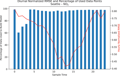
Table 4. The number of observations used to build the GAM for each site-pollutant combination. % Total Obs. is calculated as the percentage of the theoretical maximum of observations for that period. The theoretical maximum number of observations is calculated by multiplying the number of days from March 1 - May 31 by the number of hourly observations per day by the number of years for each period. Thus, the pre-COVID period has a theoretical maximum of 4416, while the COVID period has a theoretical maximum of 2208. Data is displayed on both an hourly and daily basis, where a “day” was considered to be one calendar date in which samples were recorded for at least 21 hours of the day.

* The value outside parentheses is the observed mean while the value inside parentheses is the mean of the model estimates.

As stated earlier, a log-adjusted GAM was initially considered. It performed well under a visual inspection using the hourly geometric means of the observed and estimated concentrations. However, when estimating the contribution of each vehicle class, the log-adjusted model showed a higher rate of occurrence of this potential error, ultimately leading to the selection of the non-log-adjusted model.

Using the model to estimate NO_x to CO and BC to NO_x emission ratios

The GAM approach can also be used to estimate emission ratios to help evaluate near-road pollution inventories, which similar studies using COVID-based models have not yet done (Yang et al. 2021). The GAM-estimated ratios of mobile source NO_x to CO impacts during the pre-COVID period at Queens and Seattle, which were the two cases not exhibiting implausible results, were 0.21 and 0.30 μg m⁻³ NO_x (μg m⁻³ CO)⁻¹, respectively (Table 5). These ratios were calculated by dividing the estimated total NO_x impacts from mobile sources by the estimated total CO impacts from mobile sources over the pre-COVID period. The ratios are both consistent across the COVID period as well, but the pre-COVID ratio is of the most interest in this case as it represents the typical emissions used in inventories. The emissions ratios were also estimated using the slope of an orthogonal regression line, which gave ratios of 0.25 (R²: 0.70, SE: 0.002) and 0.32 (R²: 0.83, SE: 0.002) μg m⁻³ NO_x (μg m⁻³ CO)⁻¹ in Queens and Seattle, respectively (Table 5). According to data from the NEI, the county average in 2017 was 0.16 μg m⁻³ NO_x (μg m⁻³ CO)⁻¹ in both Queens, NY and King, WA counties (United States Environmental Protection Agency 2017), considerably lower than the ratios estimated by the model. The disagreement between NEI and GAM results discussed earlier is again reflected in these ratios. A recent study by Lal, Ramaswami, and Russell estimated NO_x to CO emission ratios by comparing the differences between near-road observations and corresponding non-near road observations. Using an orthogonal regression approach like this study, they estimated an emission ratio of 0.27 μg m⁻³ NO_x (μg m⁻³ CO)⁻¹ (Lal, Ramaswami, and Russell 2020), which shows good agreement with the GAM results. The same study, however, also estimated a ratio of 0.17 μg m⁻³ NO_x (μg m⁻³ CO)⁻¹ when using the average enhancement between near-road and non-near-road measurements (Lal, Ramaswami, and Russell 2020), which agrees well with the NEI estimates and moderately with the GAM results.

Table 5. Estimated pre-COVID mobile source emission ratios at each site (with the exception of the Long Beach site, which only measured one pollutant). Ratios outside parentheses were calculated as the ratio of total emissions over the pre-COVID period, while those in parentheses represent the ratio calculated using the orthogonal regression of each wind-adjusted pollutant estimate in the pre-COVID period. The numbers in the brackets are the R-Squared value of the corresponding regression model and the standard error of the slope, respectively.

Site	BC : NOx (µg/m^3 : µg/m^3)	NOx : CO (µg/m^3 : µg/m^3)
Anaheim	–	0.09 (0.07 [0.75 | 0.001])
Atlanta	0.03 (0.034 [0.91 | 0.0])	0.16 (0.13 [0.6 | 0.002])
Oakland	0.016 (0.016 [0.98 | 0.0])	0.32 (0.3 [0.28 | 0.007])
Ontario	–	0.36 (0.4 [0.69 | 0.005])
Queens	0.017 (0.018 [0.86 | 0.0])	0.21 (0.26 [0.7 | 0.003])
Seattle	0.013 (0.017 [0.95 | 0.0])	0.3 (0.32 [0.83 | 0.002])

The GAM results can also be used to estimate mobile source BC to NO_x ratios in Oakland, Queens, and Seattle, the three sites with plausible results for both pollutants. Using the ratio of the total impacts across the pre-COVID period yields a pre-COVID BC to NO_x emission ratio of 0.016, 0.017, and 0.013 μg m⁻³ BC (μg m⁻³ NO_x)⁻¹ in the three respective cities. The orthogonal regression approach estimates ratios of 0.016, 0.018, and 0.017 μg m⁻³ BC (μg m⁻³ NO_x)⁻¹, which are consistent with the averaging approach (Table 5). As discussed previously, the NEI estimates use EC measurements instead of BC. However, because of the high correlation between EC and BC, these estimates can still be used to evaluate the GAM results. In 2017, the NEI-estimated annual mobile source EC to NO_x ratio was 0.010, 0.013, and 0.010 μg m⁻³ EC (μg m⁻³ NO_x)⁻¹ in Alameda, Queens, and King counties, the counties corresponding to the three sites. These existing estimates show relatively strong agreement with the GAM results, though the GAM is again showing a slightly higher ratio. This discrepancy could be due to the differences in EC and BC measurement but is still relatively small and provides adequate support for the GAM findings.

Conclusion

Utilizing a GAM, built with data showing traffic reductions and observed air quality changes due to COVID-19, resulted in similar LD and HD emission contribution patterns across the investigated sites. Specific contributions of both LD and HD traffic to BC, NOx, and CO near-road air pollution levels were city-dependent, as is expected given the variability of several regional factors, including other pollution sources and varying fleet composition. These site-specific GAM results found varying levels of agreement with existing NEI LD and HD traffic emissions estimates, though general contribution trends observed in the GAM estimates did agree with the NEI. For example, in general, the model found LD traffic to be a larger contributor to CO near-road impacts than HD traffic. Contributions to BC and NO_x impacts were more evenly split and varied across the different sites. In general, pandemic-era lockdowns decreased the contributions of mobile sources to urban near-road pollution levels but increased the relative percent contribution of HD traffic to mobile source impacts. This can potentially be explained by a sustained reliance on essential freight throughout the pandemic, despite decreases in non-essential commuter traffic.

However, this approach was found to have limitations. GAM-model estimated on-road mobile sources at five of the seven sites under investigation, including Atlanta, Oakland, and the three sites in the SoCAB, were found to contribute greater than 100% to total near-road impacts of at least one pollutant across a certain period. This could be a sign that the GAM used in this study did not include important confounding factors, such as non-freeway traffic. The number of observations used to build the model also seemed to indicate the success of the model, as the Seattle and Queens models were built on the largest number of observations. Despite the occasional occurrence of implausible results, building a model with sufficient hourly observations yielded moderate to strong agreement with existing mobile source contribution and emission ratio estimates, indicating that this approach is practical.

Acknowledgments

The authors acknowledge Ken Buckley, Sunni Ivey, Ziqi Gao, and Isha Khanna for their help in the research process.

Supplemental data

Supplemental data for this article can be accessed online at https://doi.org/10.1080/10962247.2023.2185315

Disclosure statement

No potential conflict of interest was reported by the author(s).

Data availability statement

The data that support the findings of this study are openly available in Open Science Framework at http://doi.org/10.17605/OSF.IO/32HQR.

Additional information

Funding

The work was supported by the Phillips 66 [No #]; NASA HAQAST [80NSSC21K0506].

Notes on contributors

Samuel Orth

Samuel Orth is a fourth-year undergraduate student pursuing his B.S. in Mechanical Engineering at Georgia Institute of Technology in Atlanta, GA.

Armistead G. Russell

Armistead G. Russell is the Howard T. Tellepsen Chair and Regents’ Professor of Civil and Environmental Engineering at Georgia Institute of Technology in Atlanta, GA.

References

- Agarwal, A. 2004. A comparison of weekend and weekday travel behavior characteristics in urban areas. M.S.C.E., Civil Engineering, University of South Florida. [Online]. https://digitalcommons.usf.edu/etd/936.
- Aldrin, M., and I. H. Haff. 2005. Generalised additive modelling of air pollution, traffic volume and meteorology. Atmos. Environ. 39 (11):2145–55. doi:10.1016/j.atmosenv.2004.12.020.
- Ambient Monitoring Technology Information Center. 2020. Near-road site list. ed. United States Environmental Protection Agency.
- Bar, S., B. R. Parida, S. P. Mandal, A. C. Pandey, N. Kumar, and B. Mishra. 2021. Impacts of partial to complete COVID-19 lockdown on NO2 and PM2.5 levels in major urban cities of Europe and USA. Elsevier Public Health Emerg. Coll. doi:10.1016/j.cities.2021.103308.
- Bauwens, M., S. Compernolle, T. Stavrakou, J.-F. Müller, J. Gent, H. Eskes, P. F. Levelt, A. R. Van Der, J. P. Veefkind, J. Vlietinck, et al. 2020. Impact of Coronavirus outbreak on NO2 pollution assessed using TROPOMI and OMI observations. SPECIAL COLLECTION: COVID-19 Pandemic: Linking Health Soc. Environ. 47 (11), May 8. doi:10.1029/2020GL087978.
- Berman, J. D., and K. Ebisu. 2020. Changes in U.S. air pollution during the COVID-19 pandemic. Sci. Total Environ. 739 (SI: COVID–19: Impact by and on the Environment, October 15, 2020). doi: 10.1016/j.scitotenv.2020.139864.
- Bick, A., A. Blandin, and K. Mertens. 2020. Work from home before and after the Covid-19 outbreak. FRB of Dallas Working Paper No. 2017. doi:10.24149/wp2017r2.
- Boriboonsomsin, K., and M. Barth. 2008. Impacts of freeway high-occupancy vehicle lane configuration on vehicle emissions. Transp. Res. D 13 (2):112–25. doi:10.1016/j.trd.2008.01.001.
- Braga, A. L. F., P. H. Saldiva, L. A. Pereira, J. J. Menezes, G. M. Conceição, C. A. Lin, A. Zanobetti, J. Schwartz, and D. W. Dockery. 2001. Health effects of air pollution exposure on children and adolescents in São Paulo, Brazil. Pediatr. Pulmonol. 31 (2):106–13, February. doi:10.1002/1099-0496(200102)31:2<106:AID-PPUL1017>3.0.CO;2-M.
- California Department of Transportation. Performance measurement system (PeMS). [Online]. https://pems.dot.ca.gov/.
- Chen, Y., R. Qin, G. Zhang, and H. Albanwan. 2021. Spatial temporal analysis of traffic patterns during the COVID-19 epidemic by vehicle detection using planet remote-sensing satellite images. Remote. Sens. 13 (2). doi: 10.3390/rs13020208.
- Cicero-Fernândez, P., J. R. Long, and A. M. Winer. 1997. Effects of grades and other loads on on-road emissions of hydrocarbons and carbon monoxide. J. Air Waste Manag. Assoc. 47 (8):898–904. doi:10.1080/10473289.1997.10464455.
- Czeisler, M. É., M. E. Howard, R. Robbins, L. K. Barger, E. R. Facer-Childs, S. M. W. Rajaratnam, and C. A. Czeisler. 2021. Early public adherence with and support for stay-at-home COVID-19 mitigation strategies despite adverse life impact: A transnational cross-sectional survey study in the United States and Australia. BMC Public Health 21:Art no. 503. doi:10.1186/s12889-021-10410-x.
- Du, J., H. A. Rakha, F. Filali, and H. Eldardiry. 2020. COVID-19 pandemic impacts on traffic system delay, fuel consumption and emissions. Int. J. Transp. Sci. Technol. 10 (2):184–96. doi:10.1016/j.ijtst.2020.11.003.
- Elshorbany, Y. F., H. C. Kapper, J. R. Ziemke, and S. A. Parr. 2021. The status of air quality in the United States during the COVID-19 pandemic: A remote sensing perspective. Remote. Sens. 13 (3):369. doi:10.3390/rs13030369.
- Emery, C., Z. Liu, A. G. Russell, M. T. Odman, G. Yarwood, and N. Kumar. 2017. Recommendations on statistics and benchmarks to assess photochemical model performance. J. Air Waste Manag. Assoc. 67 (5):582–98. doi:10.1080/10962247.2016.1265027.
- Georgia Department of Transportation. Traffic Analysis and Data Application. [Online]. https://gdottrafficdata.drakewell.com/publicmultinodemap.asp.
- Hajat, A., C. Hsia, and M. S. O’Neill. 2015. Socioeconomic disparities and air pollution exposure: A global review. Curr. Environ. Health Rep. 2:440–50. doi:10.1007/s40572-015-0069-5.
- Highway Data Services Bureau. Downloadable traffic data. [Online]. https://www.dot.ny.gov/divisions/engineering/technical-services/highway-data-services/hdsb.
- Highway Data Services Bureau. 2021. Effect of the COVID-19 pandemic on traffic in New York state in 2020. New York State Department of Transportation.
- Hoek, G., R. M. Krishnan, R. Beelen, A. Peters, B. Ostro, B. Brunekreef, and J. D. Kaufman. 2013. Long-term air pollution exposure and cardio-respiratory mortality: A review. Environ. Health 12:43. doi:10.1186/1476-069X-12-43.
- Hudda, N., M. C. Simon, A. P. Patton, and J. L. Durant. 2020. Reductions in traffic-related black carbon and ultrafine particle number concentrations in an urban neighborhood during the COVID-19 pandemic. Sci. Total Environ. 742 (Special Issue: COVID–19: Impact by and on the Environment). doi: 10.1016/j.scitotenv.2020.140931.
- Ihuoma-Walter, I. M. 2021. Multi-modal traffic signal reallocation for an intersection with high freight volumes and the impact of COVID. Doctor of Engineering, Civil Engineering, Morgan State University, Ann Arbor, 28497608. [Online]. https://go.openathens.net/redirector/gatech.edu?url=https://search.proquest.com/dissertations-theses/multi-modal-traffic-signal-reallocation/docview/2546060801/se-2?accountid=11107.
- Lal, R. M., A. Ramaswami, and A. G. Russell. 2020. Assessment of the near-road (monitoring) network including comparison with nearby monitors within US cities: New findings from nationwide observations with implications for urban environmental health outcomes. Environ. Res. Lett. 15 (11). doi: 10.1088/1748-9326/ab8156.
- Lasry, A., D. Kidder, M. Hast, J. Poovey, G. Sunshine, K. Winglee, N. Zviedrite, F. Ahmed, K. A. Ethier, C. Clodfelter, et al. 2020. Timing Of community mitigation and changes in reported COVID-19 and community mobility ― Four U.S. metropolitan areas, February 26–April 1, 2020. Morb. Mortal. Wkly. Rep. 69 (15):451–57. doi:10.15585/mmwr.mm6915e2.
- Leins, C. 2020. 10 states with the most aggressive response to COVID-19. ed. U.S. News & World Report.
- Mavroidis, I., and M. Ilia. 2012. Trends of NOx, NO2 and O3 concentrations at three different types of air quality monitoring stations in Athens, Greece. Atmos. Environ. 63:135–47, December. doi:10.1016/j.atmosenv.2012.09.030.
- McDonald, B. C., S. A. McKeen, Y. Y. Cui, R. Ahmadov, S.-W. Kim, G. J. Frost, I. B. Pollack, J. Peischl, T. B. Ryerson, J. S. Holloway, et al. 2018. Modeling ozone in the Eastern U.S. using a fuel-based mobile source emissions inventory. Environ. Sci. Technol. 52 (13):7360–70. doi:10.1021/acs.est.8b00778.
- mgcv: Mixed GAM Computation Vehicle with Automatic Smoothness Estimation. 2022. [Online]. https://cran.r-project.org/web/packages/mgcv/index.html.
- Mitchell, S. H., E. M. Bulger, H. C. Duber, A. L. Greninger, T. D. Ong, S. C. Morris, L. D. Chew, T. M. Haffner, V. L. Sakata, J. B. Lynch, et al. 2020. Western Washington State COVID-19 experience: Keys to flattening the curve and effective health system response. J. Am. Coll. Surg. 231 (3):316–24. doi:10.1016/j.jamcollsurg.2020.06.006.
- Morawska, L., E. R. Jayaratne, K. Mengersen, M. Jamriska, and S. Thomas. 2002. Differences in airborne particle and gaseous concentrations in urban air between weekdays and weekends. Atmos. Environ. 36 (27):4375–83. doi:10.1016/S1352-2310(02)00337-0.
- Mueller, D., S. Uibel, M. Takemura, D. Klingelhoefer, and D. A. Groneberg. 2011. Ships, ports, and particulate air pollution – an analysis of recent studies. J. Occup. Med. Toxicol. 6:Art no. 31. doi:10.1186/1745-6673-6-31.
- National Centers for Environmental Information, NESDIS, NOAA, and U.S. Department of Commerce. U.S. Local Climatological Data (LCD).
- New York State Department of Transportation. Traffic data viewer. [Online]. https://gisportalny.dot.ny.gov/portalny/apps/webappviewer/index.html?id=28537cbc8b5941e19cf8e959b16797b4.
- Park, Y. M., and M.-P. Kwan. 2020. Pollution: Considering the spatiotemporal dynamics of population distribution. Int J Environ Res Public Health 17 (3), February 1. doi:10.3390/ijerph17030908.
- Qin, M., H. Yu, Y. Hu, A. G. Russell, M. T. Odman, K. Doty, A. Pour-Biazar, R. T. McNider, and E. Knipping. 2019. Improving ozone simulations in the Great Lakes Region: The role of emissions, chemistry, and dry deposition. Atmos. Environ. 202:167–79. doi:10.1016/j.atmosenv.2019.01.025.
- R: A Language and Environment for Statistical Computing. 2021. Vienna, Austria: R Foundation for Statistical Computing. [Online]. https://www.R-project.org/.
- Salako, G. O., P. K. Hopke, D. D. Cohen, B. A. Begum, S. K. Biswas, G. G. Pandit, Y. -S. Chung, S. A. Rahman, M. S. Hamzah, P. Davy, et al. 2012. Exploring the variation between EC and BC in a variety of locations. Aerosol Air Qual. Res. 12 (1):1–7. doi:10.4209/aaqr.2011.09.0150.
- Schatke, M., F. Meier, B. Schröder, and S. Weber. 2022. Impact of the 2020 COVID-19 lockdown on NO2 and PM10 concentrations in Berlin, Germany. Atmos. Environ. 290. doi:10.1016/j.atmosenv.2022.119372.
- Shi, X., and G. P. Brasseur. 2020. The response in air quality to the reduction of Chinese economic activities during the COVID-19 outbreak. SPECIAL COLLECTION: COVID-19 Pandemic: Linking Health Soc. Environ. 47, May 18. doi:10.1029/2020GL088070.
- Tang, J., A. McNabola, B. Misstear, F. Pilla, and M. S. Alam. 2019. Assessing the impact of vehicle speed limits and fleet composition on air quality near a school. Int J Environ Res Public Health 16 (1). doi: 10.3390/ijerph16010149.
- Tanzer-Gruener, R., J. Li, S. R. Eilenberg, A. L. Robinson, and A. A. Presto. 2020. Impacts of modifiable factors on ambient air pollution: A case study of COVID-19 shutdowns. Environ. Sci. Technol. Lett. 7 (8):554–59. doi:10.1021/acs.estlett.0c00365.
- Tian, N., J. Xue, and T. M. Barzyk. 2012. Evaluating socioeconomic and racial differences in traffic-related metrics in the United States using a GIS approach. J. Expo. Sci. Environ. Epidemiol. 23 (2):215–22. doi:10.1038/jes.2012.83.
- United States Environmental Protection Agency. Air quality system API. United States Environmental Protection Agency. [Online]. https://aqs.epa.gov/aqsweb/documents/data_api.html.
- United States Environmental Protection Agency. 2017. 2017 National Emissions Inventory (NEI) Data. [Online]. https://www.epa.gov/air-emissions-inventories/2017-national-emissions-inventory-nei-data.
- United States Federal Highway Administration. 2014. Traffic monitoring guide. United States Federal Highway Administration.
- Washington’s Air Quality Network. Site report. [Online]. https://enviwa.ecology.wa.gov/report/SingleStationReport.
- Washington State Department of Transportation. Traffic GeoPortal. [Online]. https://www.wsdot.wa.gov/data/tools/geoportal/?config=traffic.
- Washington State Department of Transportation. 2019. Request for traffic data form. ed. Washington State Department of Transportation, 2.
- Wild, R. J., W. P. Dubé, K. C. Aikin, S. J. Eilerman, J. A. Neuman, J. Peischl, T. B. Ryerson, and S. S. Brown. 2017. On-road measurements of vehicle NO2/NOx emission ratios in Denver, Colorado, USA. Atmos. Environ. 148:182–89, January. doi:10.1016/j.atmosenv.2016.10.039.
- Wu, J., S. Smith, M. Khurana, C. Siemaszko, and B. DeJesus-Banos. 2020. Stay-at-home orders across the country. NBC, ed. NBC News.
- Wyatt, D. W., H. Li, and J. E. Tate. 2014. The impact of road grade on carbon dioxide (CO2) emission of a passenger vehicle in real-world driving. Transp. Res. D 32:160–70. doi:10.1016/j.trd.2014.07.015.
- Xiang, J., E. Austin, T. Gould, T. Larson, J. Shirai, Y. Liu, J. Marshall, and E. Seto. 2020. Impacts of the COVID-19 responses on traffic-related air pollution in a Northwestern US city. Sci. Total Environ. 747:141325, December 10. doi:10.1016/j.scitotenv.2020.141325.
- Xu, K., K. Cui, L.-H. Young, Y.-K. Hsieh, Y.-F. Wang, J. Zhang, and S. Wan. 2020. Impact of the COVID-19 event on air quality in Central China. Aerosol Air Qual. Res. (5):915–29. doi:10.4209/aaqr.2020.04.0150.
- Yang, J., Y. Wen, Y. Wang, S. Zhang, J. P. Pinto, E. A. Pennington, Z. Wang, Y. Wu, S. P. Sander, J. H. Jiang, et al. 2021. From COVID-19 to future electrification: Assessing traffic impacts on air quality by a machine-learning model. Proc. Natl. Acad. Sci. 118 (26), June 21. doi:10.1073/pnas.2102705118.