Optimization model for bus priority control considering carbon emissions

ABSTRACT

To study the impact of bus priority control (BPC) on traffic carbon emissions under the strategies of speed guidance, green extension (GE), and red truncation (RT), with consideration of the main influencing factors such as delay, stopping times, and speed, a combination optimization method was used to develop a bi-level optimization model for BPC. The optimal carbon-emission reductions of buses and social vehicles with different fuel types in the upstream section of the intersection and the intersection control area was the upper-level objective, and the optimal total passenger-delay reduction was the lower-level objective. The Gauss – Seidel iterative algorithm was used to solve the model. Finally, the model was applied to the analysis of calculation cases. The results indicated that after BPC was adopted under the guidance acceleration strategy, the reductions in the carbon emissions and total delay of passenger were optimal when the guidance speed was 38 km/h, i.e. 12.67% and 21.05%, respectively. Under the guidance acceleration and GE strategy, the reductions in the carbon emissions and total delay of passenger were optimal when the guidance speed was 39 km/h and the GE was 6 s, i.e. 27.49% and 38.62%, respectively. Under the guidance deceleration and RT strategy, the reductions in the carbon emissions and total delay of passenger were optimal when the guidance speed was 29 km/h and the RT was 6 s, i.e. 22.18% and 33.52%, respectively. The model reduced the carbon emissions and total delay of passenger in the upstream section of the intersection and the intersection control area to achieve the optimal overall traffic benefit for the intersection.

SUMMARY

1. Two bus signal priority control strategies – green extension and red truncation – were studied.

2. Carbon emission and delay calculation methods under the bus priority control were developed.

3. Considering carbon-emission reductions of buses and social vehicles with different fuel types under different working conditions.

4. Three control methods were studied: guidance acceleration, guidance acceleration and green extension, and guidance deceleration and red truncation.

Introduction

In recent years, with the increasing number of motor vehicles in China, urban traffic congestion has become a significant problem with limited road resources. Urban buses are unattractive to residents, and bus signal priority (BSP)-one of the important measures of the bus priority control (BPC) strategy – can be used to effectively reduce the delay caused by buses in the process of driving, increasing their operational efficiency; thus, it is important for reducing vehicle carbon emissions and alleviating urban traffic congestion.

In many studies, the total delay of passenger at the intersection, vehicle queue length, and intersection capacity were selected as optimization targets, and the BSP strategy was adopted to achieve bus priority at intersections. For example, Thodi, Chilukuri, and Vanajakshi (2022) adopted green extension (GE) and red truncation (RT) strategies, taking the minimum total delay of passenger in the intersection control area as the optimization goal, and used PTV Vissim software for simulation analysis. Kim, Cheng, and Chang (2018) proposed a BSP transmission model based on urban arterial roads, which considers the effects of the average bus stop time and bus stop capacity. Wunderlich et al. (2020) proposed a dynamic signal scheduling method based on the maximum weight matching algorithm with the queue length as the optimization index and realized bus priority scheduling in the longest queue direction. Parr and Kaisar (2021) proposed a multi-objective optimization model based on the coordinated control of arterial signals, aiming at reducing the intersection delay and maximizing the intersection capacity. Wahlstedt (2011) used a microsimulation model to analyze the influence of bus priority on buses and social vehicles and to shorten the travel time of buses.

In the aforementioned studies, the problem of bus priority was only solved from the perspective of signal priority. In recent years, some scholars have introduced the method of speed guidance to the field of BPC and studied the entire process of bus driving in the upstream section of the intersection and intersection control area. For example, Ceylan and Bell (2020) adopted the speed guidance control mode and developed a BSP timing model based on a genetic algorithm with delay and stopping times as the optimization objectives. Ou, Yu, and Wa (2022) realized the integrated control of speed guidance, station control, and signal priority based on the strategy of speed guidance and BSP with the goal of minimizing the delay of social vehicles. Bie et al. (2020) developed a bus travel time prediction model with dynamic control by adopting speed guidance and a signal-priority strategy.

With increasing emphasis on carbon emissions, research on the optimization of carbon emissions in bus signal priority control (BSPC) has achieved certain results. Kwak, Park, and Lee (2019) believed that the setting of traffic signal parameters can significantly affect the delay and carbon emissions of vehicles at signal intersections, and the optimal traffic signal timing can reduce traffic carbon emissions by 8%–20%. Karekla, Fernandez, and Tyler (2018) developed a BSP control model considering indicators such as the bus energy consumption and carbon emissions and solved it using a genetic algorithm. Hallmark et al. (2020) used a decision optimization model to analyze and calculate carbon emissions and demonstrated that signal assignment can affect carbon emissions in a road network.

As indicated by the literature, in most previous studies, the delay, queue length, and intersection capacity were taken as the optimization objectives of the model, and there have been few studies in which the effects of carbon emissions and delay on BPC strategies were considered simultaneously under the concept of emission peak and carbon neutrality. In most previous studies, BSP was achieved by establishing a single-objective or multi-objective optimization model. However, in a multi-objective optimization model, the weight value of the optimization goal is subjective, which makes the optimization result of the model inaccurate. Thus, in the present study, we developed a bi-level optimization model for BPC based on the concept of systematic optimization of intersections, using a combined control strategy of speed guidance and BSP for buses and cars of different fuel types, with the goal of optimal carbon emissions and total passenger-delay reduction in the upstream section of the intersection as well as the intersection control area. The BSP was optimized and improved.

Problem description

Using the BSP strategy to reduce traffic carbon emissions and bus delays is an effective measure to reduce ecological deterioration and improve the travel attractiveness of urban residents. Considering the effects of the main parameters, such as the delay, stopping times, and speed, on traffic carbon emissions, the combined control strategy of speed guidance and BSP was selected for the upstream section of the intersection and the intersection control area. For buses and cars with different fuel types, the carbon emissions and delays in the priority and non-priority phases were analyzed. With the optimal carbon-emission reductions as the upper-level objective and the optimal delay reduction as the lower-level objective, a bi-level optimization model for BPC was developed to optimize the intersection signal control scheme. Under the premise of ensuring that the maximum green-light extension time or red-light shortening time is not exceeded, bus is given priority to pass through the intersection stop line without stopping, and maximize the benefits of social vehicles, so as to improve the road capacity of the intersection. The BPC process is illustrated in Figure 1.

Figure 1. BPC process.

To reflect the essential problem of the model, we made the following assumptions for the developed BPC optimization model:

1. Bus driving in the bus lane, its driving speed can be freely adjusted within the limited speed range, and the bus driver can drive according to the guidance speed.

2. All buses are equipped with intelligent terminal devices with vehicle speed monitoring, location monitoring, and instant messaging functions.

3. For buses, there are only pure electric and natural-gas buses; for social vehicles, there are only pure electric and fuel cars. The effects of pedestrians and non-motor vehicles are ignored.

4. A maximum of a priority phase is executed in a signal cycle to avoid loss of green time due to excessive execution of priority phases.

5. There is no bus stop between the detector at the upstream section of the intersection and the intersection stop line.

6. Automatic cars with automatic start-stop function are not considered.

Mechanism analysis of traffic carbon emissions at signal-controlled intersections

Calculation of traffic carbon emissions under typical characteristics

A certain amount of energy is consumed in the power production process, which generates carbon emissions, and the unit energy consumption and carbon-emission coefficients differ among vehicles of different fuel types. Therefore, in this study, the vehicles were divided into electric vehicles, natural-gas vehicles, and fuel vehicles, and the traffic carbon emissions under typical characteristics were calculated according to the durations of acceleration, deceleration, idle, and constant-speed driving of vehicles at intersections (Ghafari and Akbarzadeh 2021).

(1) Deceleration carbon emissions

When the vehicle arrives at the intersection and the signal light is red, the vehicle must slow down. The calculation formula for the carbon emissions generated during the deceleration process is

(1) $E_1^p=\frac{v^p}{a_1^p}\cdot F{C}_1^p\cdot E{F}^p$(1)

where $E_1^p$ represents the carbon emissions generated during the deceleration process, $v^p$ represents the initial speed of different fuel-type vehicles arriving at the intersection,$a_1^p$ represents the braking acceleration of different fuel-type vehicles, $F{C}_1^p$ represents the energy-consumption rate of different fuel-type vehicles during deceleration, and $E{F}^p$ represents the carbon-emission factor of different fuel-type vehicles. Here, p = 1 denotes an electric vehicle, p = 2 denotes a natural-gas vehicle, and p = 3 denotes a fuel vehicle.

(2) Acceleration carbon emissions

When the green light turns on, the vehicle starts to accelerate. The calculation formula for the carbon emissions generated during the acceleration process is

(2) $E_2^p=\frac{v^p}{a_2^p}\cdot F{C}_2^p\cdot E{F}^p$(2)

where $E_2^p$ represents the carbon emissions generated during the acceleration process, $a_2^p$ represents the starting acceleration of different fuel-type vehicles, and $F{C}_2^p$ represents the energy-consumption rate of different fuel-type vehicles during acceleration.

(3) Idle carbon emissions

Before the green light turns on, vehicles must stop and wait. The calculation formula for the carbon emissions generated during the stop-and-wait process is

(3) $E_3^p=t_1^p\cdot F{C}_3^p\cdot E{F}^p$(3)

where $E_3^p$ represents the carbon emissions generated during the stop-and-wait process, $t_1^p$ represents the idle time of different fuel-type vehicles, and $F{C}_3^p$ represents the energy-consumption rate of different fuel-type vehicles in the idle state.

(4) Constant-speed carbon emissions

The process of the vehicle returning to the initial speed and leaving the stop line at the intersection is called the constant-speed driving process. The calculation formula for the carbon emissions generated during the constant-speed driving process is

(4) $E_4^p=\frac{d-\frac{{\left(v^p\right)}^2}{2\cdot a_1^p}-\frac{{\left(v^p\right)}^2}{2\cdot a_2^p}}{v^p}\cdot F{C}_4^p\cdot E{F}^p$(4)

where $E_4^p$ represents the carbon emissions generated during the constant-speed driving process, d represents the distance from the first stop of the vehicle to the stop line, and $F{C}_4^p$ represents the energy-consumption rate of different fuel-type vehicles at a constant speed.

In summary, the carbon emissions generated by a vehicle arriving at the intersection and leaving the stop line (${\mathit{\text{E}}}^{\text{‘}}$) are given as

(5) $E^{\prime }=\sum _{p=1}^3{E}_1^p+E_2^p+E_3^p+E_4^p$(5)

Effects of main parameters on traffic carbon emissions

Effect of delay on carbon emission

The delay of vehicles in the upstream section of the intersection, as well as the intersection control area, can be divided into deceleration, acceleration, and idle delays (Anser et al. 2021; Hu et al. 2022), and the carbon emissions under different delays are calculated as follows:

(1) Carbon emissions under deceleration delay

When a vehicle arrives at an intersection and encounters a signal with a red-light state, the vehicle must slow down, resulting in a deceleration delay. Considering the impact of the deceleration delay, the calculation formula for the changed carbon emissions is

(6) $F_1^p=\left(\frac{v^p}{a_1^p}\cdot F{C}_1^P-\frac{v^p}{2a_1^p}\cdot F{C}_4^P\right)\cdot E{F}^p$(6)

where $F_1^p$ represents the carbon emissions under the deceleration delay.

(2) Carbon emissions under acceleration delay

When the signal light turns green, the vehicle starts to accelerate away from the intersection, resulting in an acceleration delay. Considering the effect of the acceleration delay, the calculation formula for the changed carbon emissions is

(7) $F_2^p=\left(\frac{v^p}{a_2^p}\cdot F{C}_2^P-\frac{v^p}{2a_2^p}\cdot F{C}_4^P\right)\cdot E{F}^p$(7)

where $F_2^p$ represents the carbon emissions under the acceleration delay.

(3) Carbon emissions under idle delay

In the process of stopping and waiting, idle delays occur. Considering the effect of the idle delay, the calculation formula for the changed carbon emissions is

(8) $F_3^p=\left(D-\frac{v^p}{2a_1^p}-\frac{v^p}{2a_2^p}\right).F{C}_3^p\cdot E{F}^p$(8)

where $F_3^p$ represents the carbon emissions under the idle delay, and D represents the total delay caused by vehicle driving.

Impact of stopping times on carbon emission

Considering that the vehicle stops several times during the process of passing through the intersection, the number of accelerations and decelerations of the vehicle change with different stopping times, leading to a change in the carbon emissions during the process of passing through the intersection (Hu, Long, and Zhu 2016). The carbon emissions for the corresponding stopping times were calculated as follows:

Herein, the term “stopping times” refers to the stopping times of vehicles under the influence of signal control when they pass through an intersection. The formula for calculating the average stopping times of vehicles in phase i is

(9) $h_i=\sum _{j=1}^{f}0.9\cdot \frac{C-g_{ei}}{1-y_{i,\hspace{0.17em}\alpha }}$(9)

where $g_{ei}$ represents the effective green-light time of phase i, C represents the signal cycle time, $y_{i,\alpha }$ represents the flow ratio of the α^th inlet channel of phase i, and f represents the number of inlet channels.

Accordingly, the formula for calculating the average stopping times of each vehicle in a cycle is

(10) $H=\sum _{i=1}^n{h}_i\cdot q_i/\sum _{i=1}^n{q}_i$(10)

where $q_i$ represents the actual traffic volume of phase i, and n represents the number of phases.

(1) Vehicle deceleration carbon emissions

When a vehicle passes through an intersection, assuming that the average stopping times are H, the calculation formula for the carbon emissions during the deceleration process is

(11) $G_1^p=\frac{v^p}{a_1^p}\cdot F{C}_1^{{}^p}\cdot E{F}^p\cdot H$(11)

where $G_1^p$ represents the deceleration carbon emissions under the effect of the stopping times.

(2) Vehicle acceleration carbon emissions

Similarly, the calculation formula for the carbon emissions during the acceleration process is

(12) $G_2^p=\frac{v^p}{a_2^p}\cdot F{C}_2^p\cdot E{F}^p\cdot H$(12)

where $G_2^p$ represents acceleration carbon emission under the effect of the stopping times.

Impact of speed on carbon emission

As the power of the vehicle changes with respect to the vehicle speed, the unit energy consumption first decreases and then increases with an increase in vehicle speed r (Ghosh, Bhattacharyya, and Maitra 2022; Hussain, Khan, and Shaheen 2022), which leads to different carbon emissions per unit mileage for vehicles of different fuel types under different driving speeds. The calculation formula for the carbon emissions generated by vehicles of different fuel types during constant-speed driving is

(13) $\begin{array}{rl}& Q=\frac{L}{v_{\mathrm{b}1}^1}\cdot F{C}_{\mathrm{b}1}^1\cdot E{F}_1+\frac{L}{v_{\mathrm{b}2}^1}\cdot F{C}_{\mathrm{b}2}^1\cdot E{F}_2+\frac{L}{v_{\mathrm{c}1}^0}\cdot F{C}_{\mathrm{c}1}^1\cdot E{F}_1\\ & +\frac{L}{v_{\mathrm{c}2}^0}\cdot F{C}_{\mathrm{c}2}^1\cdot E{F}_3\end{array}$(13)

Here,

(14) $\left\{\begin{array}{c}F{C}_{b1}^1=6.10\mathrm{E}-5\cdot {\left(v_{b1}^1\right)}^2-4.61\mathrm{E}-3\cdot v_{b1}^1+0.22\\ F{C}_{b2}^1=4.28\mathrm{E}-4\cdot {\left(v_{b2}^1\right)}^2-3.81\mathrm{E}-2\cdot v_{b2}^1+1.09\\ F{C}_{c1}^1=1.79\mathrm{E}-5\cdot {\left(v_{c1}^0\right)}^2-1.38\mathrm{E}-3\cdot v_{c1}^0+0.07\\ F{C}_{c2}^1=2.10\mathrm{E}-5.{\left(v_{c2}^0\right)}^2-3.47\mathrm{E}-3\cdot v_{c2}^0+0.26\end{array}\right.$(14)

Q represents the carbon emissions during constant-speed driving; L represents the constant-speed driving distance; $v_{\mathrm{b}1}^1$ and $v_{\mathrm{b}2}^1$ represent the driving speeds of pure electric and natural-gas buses, respectively; $F{C}_{\mathrm{b}1}^1$ and $F{C}_{\mathrm{b}2}^1$ represent the energy-consumption rates of pure electric and natural-gas buses, respectively, under a constant speed; $F{C}_{\mathrm{c}1}^1$ and $F{C}_{\mathrm{c}2}^1$ represent the energy-consumption rates of pure electric and fuel cars, respectively, under a constant speed; and $E{F}_1$, $E{F}_2$, and $E{F}_3$ represent the carbon-emission factors of electric vehicles, natural-gas vehicles, and fuel vehicles, respectively.

Optimization model for BPC considering carbon emissions

Speed guidance and BSPC strategies aim to reduce carbon emissions and respond to sustainable development while reducing passenger-delays in the upstream section of the intersection and the intersection control area. Because the power of a vehicle changes with respect to its speed, the carbon emissions per unit mileage vary with different guidance speeds (Chłopek et al. 2018). Therefore, the combination optimization method was used to develop a bi-level optimization model for BPC with the optimal carbon-emission reductions as the upper-level objective and the optimal total passenger-delay reduction as the lower-level objective.

Upper-level model based on carbon-emission control

(1) Guidance acceleration

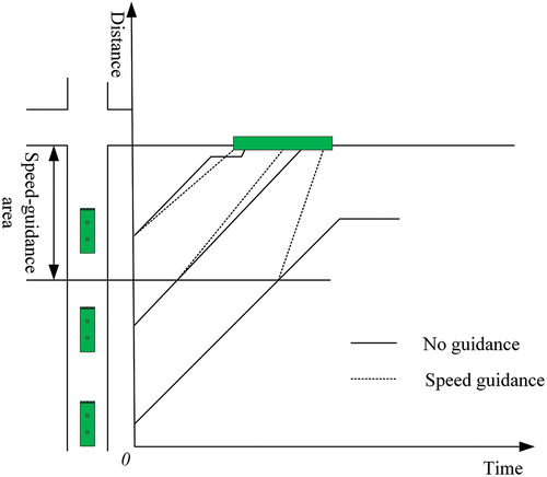
In the upstream section of the intersection, when the bus enters the speed-guidance area, the remaining green-light time of the phase cannot meet the requirement for the bus to pass through the stop line at the intersection, that is, $v_0\cdot t_{\mathrm{g}}<L_{\mathrm{b}}$. When the guidance acceleration strategy is adopted, the bus can smoothly pass through the stop line during the remaining green-light time; that is, $\left(v_1^2-v_0^2\right)/2a_2+v_1\cdot \left[t_{\mathrm{g}}-\left(v_1-v_0\right)/a_2\right]\ge L_{\mathrm{b}}$. The implementation effect of the speed guidance strategy is shown in Figure 2.

Figure 2. Schematic of the speed guidance strategy.

The calculation formula for the carbon-emission reductions of pure electric and natural-gas buses under the guidance acceleration strategy is

(15) $\left\{\begin{array}{c}\mathrm{\Delta }{E}_{\mathrm{b}1}^1=\left(\frac{L_{\mathrm{b}}}{v_{\mathrm{b}1}^0}-\frac{L_{\mathrm{b}}}{v_{\mathrm{b}1}^1}\right).F{C}_{\mathrm{b}1}^1\cdot E{F}_1\\ \mathrm{\Delta }{E}_{\mathrm{b}2}^1=\left(\frac{L_{\mathrm{b}}}{v_{\mathrm{b}2}^0}-\frac{L_{\mathrm{b}}}{v_{\mathrm{b}2}^1}\right).F{C}_{\mathrm{b}2}^1\cdot E{F}_2\end{array}\right.$(15)

where $\mathrm{\Delta }{E}_{\mathrm{b}1}^1$ and $\mathrm{\Delta }{E}_{\mathrm{b}2}^1$ represent the carbon-emission reductions of a pure electric bus and natural-gas bus, respectively, when the guidance acceleration strategy is adopted; $v_{\mathrm{b}1}^0$ and $v_{\mathrm{b}2}^0$ represent the initial speeds of the pure electric and natural-gas buses, respectively; and $v_{\mathrm{b}1}^1$ and $v_{\mathrm{b}2}^1$ represent the guidance speed of the pure electric and natural-gas buses, respectively.

Accordingly, the calculation formula for the carbon-emission reductions when the guidance acceleration strategy is adopted is

(16) $\mathrm{\Delta }{E}_1=\mathrm{\Delta }{E}_{\mathrm{b}1}^1+\mathrm{\Delta }{E}_{\mathrm{b}2}^1$(16)

(2) Guidance acceleration and GE

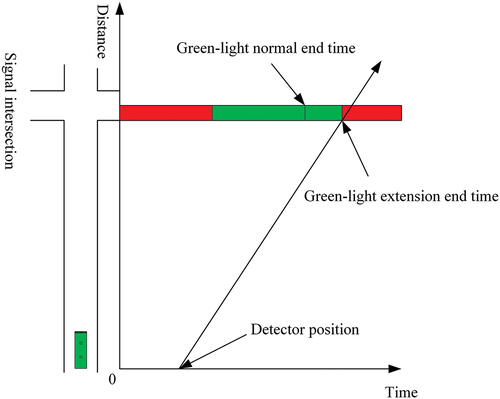
GE is a bus active priority control strategy. It is described as follows: when the bus applied for the priority phase cannot pass through the stop line at the intersection within the remaining green-light time, the green-light time of this phase can be extended to allow it to pass through the intersection without stopping (Hasan et al. 2021) to avoid the stop-start and queuing processes. The implementation effect of the GE strategy is shown in Figure 3.

Figure 3. Schematic of the GE strategy.

If the remaining green-light time of the bus priority phase is still unable to meet the requirement for the bus passing through the intersection stop line when the guidance acceleration strategy is used, that is, $\left(v_1^2-v_0^2\right)/2a_2+v_1\cdot \left[t_{\mathrm{g}}-\left(v_1-v_0\right)/\left(a_2\right)\right]<L_{\mathrm{b}}$, the guidance acceleration and GE strategies can be adopted to enable the bus to pass through the stop line at the intersection without stopping, that is, $\left(v_1^2-v_0^2\right)/2a_2+v_1\cdot \left[t_{\mathrm{g}}+g_{\mathrm{e}}-\left(v_1-v_0\right)/a_2\right]\ge L_{\mathrm{b}}$. In contrast, if $\left(v_1^2-v_0^2\right)/2a_2+v_1\cdot \left[t_{\mathrm{g}}+g_{\mathrm{e}}-\left(v_1-v_0\right)/a_2\right]<L_{\mathrm{b}}$, the bus priority strategy cannot be used to enable buses to pass through the intersection without stopping. The change in carbon emissions caused by the adoption of the GE strategy at intersections mainly includes two parts: carbon-emission reductions in the bus priority phase and carbon-emission increases in the non-bus priority phase. In the above inequalities, $g_{\mathrm{e}}$ represents the green-light extension time of the priority phase.

(a) Carbon-emission reductions in bus priority phase

When the GE strategy is adopted, the carbon emissions reduced by the pure electric bus and natural-gas bus in the intersection control area can be divided into additional carbon emissions from stop-start and queuing. The calculation formula is

(17) $\left\{\begin{array}{c}\mathrm{\Delta }{E}_{\mathrm{b}1}^2=\left[\left(\frac{v_{\mathrm{b}1}^1}{a_1}\cdot F{C}_{\mathrm{b}1}^2-\frac{v_{\mathrm{b}1}^1}{2a_1}\cdot F{C}_{\mathrm{b}1}^1\right)\cdot h_i+\left(\frac{v_{\mathrm{b}1}^1}{a_2}\cdot F{C}_{\mathrm{b}1}^3-\frac{v_{\mathrm{b}1}^1}{2a_2}\cdot F{C}_{\mathrm{b}1}^1\right)\cdot h_i+\left(r_1-g_{\mathrm{e}}\right)\cdot F{C}_{\mathrm{b}1}^4\right]\cdot E{F}_1\\ \mathrm{\Delta }{E}_{\mathrm{b}2}^2=\left[\left(\frac{v_{\mathrm{b}2}^1}{a_1}\cdot F{C}_{\mathrm{b}2}^2-\frac{v_{\mathrm{b}2}^1}{2a_1}\cdot F{C}_{\mathrm{b}2}^1\right)\cdot h_i+\left(\frac{v_{b2}^1}{a_2}\cdot F{C}_{\mathrm{b}2}^3-\frac{v_{\mathrm{b}2}^1}{2a_2}\cdot F{C}_{\mathrm{b}2}^1\right)\cdot h_i+\left(r_1-g_{\mathrm{e}}\right)\cdot F{C}_{\mathrm{b}2}^4\right]\cdot E{F}_2\end{array}\right.$(17)

where $\mathrm{\Delta }{E}_{\mathrm{b}1}^2$ and $\mathrm{\Delta }{E}_{\mathrm{b}2}^2$ represent the carbon-emission reductions of pure electric and natural-gas buses, respectively, under the GE strategy; $F{C}_{\mathrm{b}1}^2$ and $F{C}_{\mathrm{b}2}^2$ represent the energy-consumption rates of the pure electric and natural-gas buses, respectively, during deceleration; $F{C}_{\mathrm{b}1}^3$ and $F{C}_{\mathrm{b}2}^3$ represent the energy-consumption rates of the pure electric and natural-gas buses, respectively, during acceleration; $F{C}_{\mathrm{b}1}^4$ and $F{C}_{\mathrm{b}2}^4$ represent the energy-consumption rates of the pure electric and natural-gas buses, respectively, during idling; r₁ represents the red-light time under the initial timing scheme for each phase; and $h_i$ represents the average stopping times of vehicles in the bus priority phase i.

When the GE strategy is adopted, not only the carbon emissions of buses are reduced, but the carbon emissions of pure electric and fuel cars in bus priority phase are reduced, too. The formula for calculating the carbon-emission reductions is

(18) $\left\{\begin{array}{c}\mathrm{\Delta }{E}_{\mathrm{c}1}^1=E{F}_1\cdot \left\{\begin{array}{c}\sum _{\beta =1}^e{q}_{\mathrm{c}1,\beta }\cdot g_{\mathrm{e}}\cdot \left[\left(\frac{v_{\mathrm{c}1}^0}{a_{\mathrm{c}1}}\cdot F{C}_{\mathrm{c}1}^2-\frac{v_{\mathrm{c}1}^0}{2a_{\mathrm{c}1}}\cdot F{C}_{\mathrm{c}1}^1\right)\cdot h_i+\left(\frac{v_{\mathrm{c}1}^0}{a_{\mathrm{c}2}}\cdot F{C}_{\mathrm{c}1}^3-\frac{v_{\mathrm{c}1}^0}{2a_{\mathrm{c}2}}\cdot F{C}_{\mathrm{c}1}^1\right)\cdot h_i\right]\\ +\sum _{\beta =1}^{e}F{C}_{\mathrm{c}1}^4\cdot \left[\frac{q_{\mathrm{c}1,\beta }}{q_{\mathrm{c}1,\beta }+q_{\mathrm{c}2,\beta }}\cdot \mathrm{\Delta }{D}_{c1,\beta }-\left(\frac{v_{\mathrm{c}1}^0}{2a_{\mathrm{c}1}}+\frac{v_{\mathrm{c}1}^0}{2a_{\mathrm{c}2}}\right)\cdot h_i\cdot q_{\mathrm{c}1,\beta }\cdot g_{\mathrm{e}}\right]\end{array}\right\}\\ \mathrm{\Delta }{E}_{\mathrm{c}2}^1=E{F}_3\cdot \left\{\begin{array}{c}\sum _{\beta =1}^e{q}_{\mathrm{c}2,\beta }\cdot g_{\mathrm{e}}\cdot \left[\left(\frac{v_{\mathrm{c}2}^0}{a_{\mathrm{c}1}}\cdot F{C}_{\mathrm{c}2}^2-\frac{v_{\mathrm{c}2}^0}{2a_{\mathrm{c}1}}\cdot F{C}_{\mathrm{c}2}^1\right)\cdot h_i+\left(\frac{v_{\mathrm{c}2}^0}{a_{\mathrm{c}2}}\cdot F{C}_{\mathrm{c}2}^3-\frac{v_{\mathrm{c}2}^0}{2a_{\mathrm{c}2}}\cdot F{C}_{\mathrm{c}2}^1\right)\cdot h_i\right]\\ +\sum _{\beta =1}^{e}F{C}_{\mathrm{c}2}^4\cdot \left[\frac{q_{\mathrm{c}2,\beta }}{q_{\mathrm{c}1,\beta }+q_{\mathrm{c}2,\beta }}\cdot \mathrm{\Delta }{D}_{c1,\beta }-\left(\frac{v_{\mathrm{c}2}^0}{2a_{\mathrm{c}1}}+\frac{v_{\mathrm{c}2}^0}{2a_{\mathrm{c}2}}\right)\cdot h_i\cdot q_{\mathrm{c}2,\beta }\cdot g_{\mathrm{e}}\right]\end{array}\right\}\end{array}\right.$(18)

where $\mathrm{\Delta }{E}_{\mathrm{c}1}^1$ and $\mathrm{\Delta }{E}_{\mathrm{c}2}^1$ represent the carbon-emission reductions of pure electric and fuel cars, respectively, in the bus priority phase when the GE strategy is adopted; $v_{\mathrm{c}1}^0$ and $v_{\mathrm{c}2}^0$ represent the initial speed of pure electric and fuel cars, respectively, at the intersection; $a_{\mathrm{c}1}$ and $a_{\mathrm{c}2}$ represent the braking acceleration and starting acceleration, respectively, of cars at the intersection; $\mathrm{\Delta }{D}_{\mathrm{c}1,\beta }$ represents the delay reduction of social vehicles in bus priority phase lane β; $q_{\mathrm{c}1,\beta }$ and $q_{\mathrm{c}2,\beta }$ represent the arrival rates of pure electric and fuel cars, respectively, in bus priority phase lane β;$F{C}_{\mathrm{c}1}^1$ and $F{C}_{\mathrm{c}2}^1$ represent the energy-consumption rates of pure electric and fuel cars, respectively, with a constant speed; $F{C}_{\mathrm{c}1}^2$ and $F{C}_{\mathrm{c}2}^2$ represent the energy-consumption rates of pure electric and fuel cars, respectively, during deceleration; $F{C}_{\mathrm{c}1}^3$ and $F{C}_{\mathrm{c}2}^3$ represent the energy-consumption rates of pure electric and fuel cars, respectively, during acceleration; and $F{C}_{\mathrm{c}1}^4$ and $F{C}_{\mathrm{c}2}^4$ represent the energy-consumption rates of pure electric and fuel cars, respectively, during idling.

(b) Carbon-emission increase in non-bus priority phase

For the non-bus priority phase, after the GE strategy is adopted, the delays of the non-priority phase pure electric and fuel cars increase, increasing the carbon emissions at intersections. The calculation formula for the increased carbon emissions is

(19) $\left\{\begin{array}{c}\mathrm{\Delta }{E}_{\mathrm{c}1}^2=E{F}_1\cdot \left\{\begin{array}{c}\sum _{k=1}^n\sum _{j=1}^m{q}_{c1,j}^k\cdot g_{\mathrm{e}}^k\cdot \left[\left(\frac{v_{\mathrm{c}1}^0}{a_{\mathrm{c}1}}\cdot F{C}_{\mathrm{c}1}^2-\frac{v_{\mathrm{c}1}^0}{2a_{\mathrm{c}1}}\cdot F{C}_{\mathrm{c}1}^1\right)\cdot h_k+\left(\frac{v_{\mathrm{c}1}^0}{a_{\mathrm{c}2}}\cdot F{C}_{\mathrm{c}1}^3-\frac{v_{\mathrm{c}1}^0}{2a_{\mathrm{c}2}}\cdot F{C}_{\mathrm{c}1}^1\right)\cdot h_k\right]\\ +\sum _{k=1}^n\sum _{j=1}^{m}F{C}_{\mathrm{c}1}^4\cdot \left[\frac{q_{\mathrm{c}1,j}^k}{q_{\mathrm{c}1,j}^k+q_{\mathrm{c}2,j}^k}\cdot \mathrm{\Delta }{D}_{\mathrm{c}2,j}^k-\left(\frac{v_{\mathrm{c}1}^0}{2a_{\mathrm{c}1}}+\frac{v_{\mathrm{c}1}^0}{2a_{\mathrm{c}2}}\right)\cdot h_k\cdot q_{\mathrm{c}1,j}^k\cdot g_{\mathrm{e}}^k\right]\end{array}\right\}\\ \mathrm{\Delta }{E}_{\mathrm{c}2}^2=E{F}_3\cdot \left\{\begin{array}{c}\sum _{k=1}^n\sum _{j=1}^m{q}_{\mathrm{c}2,j}^k\cdot g_{\mathrm{e}}^k\cdot \left[\left(\frac{v_{\mathrm{c}2}^0}{a_{\mathrm{c}1}}\cdot F{C}_{\mathrm{c}2}^2-\frac{v_{\mathrm{c}2}^0}{2a_{\mathrm{c}1}}\cdot F{C}_{\mathrm{c}2}^1\right)\cdot h_k+\left(\frac{v_{\mathrm{c}2}^0}{a_{\mathrm{c}2}}\cdot F{C}_{\mathrm{c}2}^3-\frac{v_{\mathrm{c}2}^0}{2a_{\mathrm{c}2}}\cdot F{C}_{\mathrm{c}2}^1\right)\cdot h_k\right]\\ +\sum _{k=1}^n\sum _{j=1}^{m}F{C}_{\mathrm{c}2}^4\cdot \left[\frac{q_{c2,j}^k}{q_{\mathrm{c}1,j}^k+q_{\mathrm{c}2,j}^k}\cdot \mathrm{\Delta }{D}_{\mathrm{c}2,j}^k-\left(\frac{v_{\mathrm{c}2}^0}{2a_{\mathrm{c}1}}+\frac{v_{\mathrm{c}2}^0}{2a_{\mathrm{c}2}}\right)\cdot h_k\cdot q_{\mathrm{c}2,j}^k\cdot g_{\mathrm{e}}^k\right]\end{array}\right\}\end{array}\right.$(19)

where $\mathrm{\Delta }{E}_{\mathrm{c}1}^2$ and $\mathrm{\Delta }{E}_{\mathrm{c}2}^2$ represent the carbon-emission increases of the non-bus priority phase for pure electric and fuel cars, respectively, when the GE strategy is adopted; $g_{\mathrm{e}}^k$ represents the compressed green-light time of non-bus priority phase k; $\mathrm{\Delta }{D}_{\mathrm{c}2,j}^k$ represents the increased delay of social vehicles in non-bus priority phase k lane j; and $h_k$ represents the average stopping times of vehicles in non-bus priority phase k.

Therefore, when the GE strategy is adopted, the calculation formula for the carbon-emission reductions is

(20) $\mathrm{\Delta }{E}_2=\mathrm{\Delta }{E}_{\mathrm{b}1}^2+\mathrm{\Delta }{E}_{\mathrm{b}2}^2+\mathrm{\Delta }{E}_{\mathrm{c}1}^1+\mathrm{\Delta }{E}_{\mathrm{c}2}^1-\mathrm{\Delta }{E}_{\mathrm{c}1}^2-\mathrm{\Delta }{E}_{c2}^2$(20)

where $\mathrm{\Delta }{E}_2$ represents the carbon-emission reductions when the GE strategy is adopted.

When the combination strategy of guidance acceleration and GE is adopted, the carbon-emission reductions are given as

(21) $\mathrm{\Delta }{E}^{\prime }=\mathrm{\Delta }{E}_1+\mathrm{\Delta }{E}_2$(21)

(3) Guidance deceleration and RT

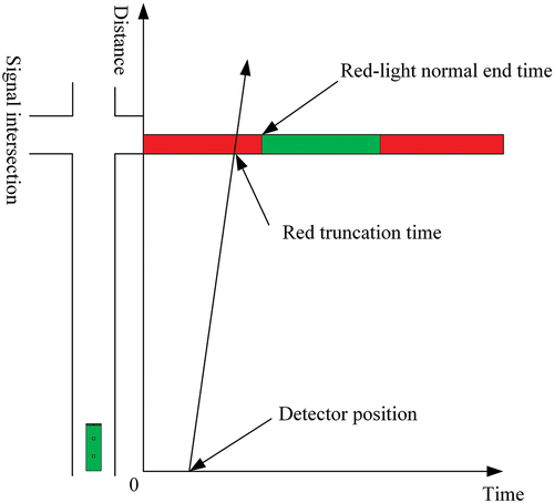
RT is also an active control strategy for bus priority. It is described as follows: when the detector monitors a priority application from a bus and predicts that the phase will be in the red phase when it arrives at the intersection stop line, the red phase can be truncated, and the green phase can be started so that the bus can pass through the intersection without stopping r (Girijan, Vanajakshi, and Chilukuri 2021; Koehler et al. 2018). The implementation effect of the RT strategy is shown in Figure 4.

Figure 4. Schematic of the RT strategy.

If the bus arrives early, the guidance deceleration strategy can be adopted to extend the time when the bus arrives at the stop line at the intersection and cooperate with the RT strategy to make $\left(v_0^2-v_2^2\right)/2a_1+v_2\cdot \left[t_{\mathrm{r}}-r_2-\left(v_0-v_2\right)/a_1\right]\le L_{\mathrm{b}}$; otherwise, the strategy will not be adopted. The change in carbon emissions generated by the RT strategy at intersections includes two parts: carbon-emission reductions in the bus priority phase and carbon-emission increases in the non-bus priority phase. In the above inequality, $t_{\mathrm{r}}$ represents the remaining red-light time, r₂ represents the red-light shortening time, and $v_2$ represents the driving speed after guidance deceleration.

(a) Carbon-emission reduction in bus priority phase

After the RT strategy is adopted, the carbon-emission reductions of pure electric and natural-gas buses in the intersection control area can be divided into additional carbon emissions from stop-start and queuing. The calculation formula is

(22) $\left\{\begin{array}{c}\mathrm{\Delta }{E}_{\mathrm{b}1}^3=\left[\left(\frac{v_{\mathrm{b}1}^1}{a_1}\cdot F{C}_{\mathrm{b}1}^2-\frac{v_{\mathrm{b}1}^1}{2a_1}\cdot F{C}_{\mathrm{b}1}^1\right)\cdot h_i+\left(\frac{v_{\mathrm{b}1}^1}{a_2}\cdot F{C}_{\mathrm{b}1}^3-\frac{v_{\mathrm{b}1}^1}{2a_2}\cdot F{C}_{\mathrm{b}1}^1\right)\cdot h_i+r_2\cdot F{C}_{\mathrm{b}1}^4\right]\cdot E{F}_1\\ \mathrm{\Delta }{E}_{\mathrm{b}2}^3=\left[\left(\frac{v_{\mathrm{b}2}^1}{a_1}\cdot F{C}_{\mathrm{b}2}^2-\frac{v_{\mathrm{b}2}^1}{2a_1}\cdot F{C}_{\mathrm{b}2}^1\right)\cdot h_i+\left(\frac{v_{\mathrm{b}2}^1}{a_2}\cdot F{C}_{\mathrm{b}2}^3-\frac{v_{\mathrm{b}2}^1}{2a_2}\cdot F{C}_{b2}^1\right)\cdot h_i+r_2\cdot F{C}_{\mathrm{b}2}^4\right]\cdot E{F}_2\end{array}\right.$(22)

where $\mathrm{\Delta }{E}_{\mathrm{b}1}^3$ and $\mathrm{\Delta }{E}_{\mathrm{b}2}^3$ represent the carbon-emission reductions of the pure electric and natural-gas buses, respectively, under the RT strategy.

Similarly, when the RT strategy is adopted, the carbon emissions of pure electric and fuel cars in the same priority phase as buses will be reduced. The calculation formula for the carbon-emission reductions is

(23) $\left\{\begin{array}{c}\mathrm{\Delta }{E}_{\mathrm{c}1}^3=E{F}_1\cdot \left\{\begin{array}{c}\sum _{\beta =1}^e{q}_{\mathrm{c}1,\beta }\cdot r_2\cdot \left[\left(\frac{v_{\mathrm{c}1}^0}{a_{\mathrm{c}1}}\cdot F{C}_{\mathrm{c}1}^2-\frac{v_{\mathrm{c}1}^0}{2a_{\mathrm{c}1}}\cdot F{C}_{\mathrm{c}1}^1\right)\cdot h_i+\left(\frac{v_{\mathrm{c}1}^0}{a_{\mathrm{c}2}}\cdot F{C}_{\mathrm{c}1}^3-\frac{v_{\mathrm{c}1}^0}{2a_{\mathrm{c}2}}\cdot F{C}_{\mathrm{c}1}^1\right)\cdot h_i\right]\\ +\sum _{\beta =1}^{e}F{C}_{\mathrm{c}1}^4\cdot \left[\frac{q_{c1,\beta }}{q_{\mathrm{c}1,\beta }+q_{\mathrm{c}2,\beta }}\cdot \mathrm{\Delta }{D}_{\mathrm{c}3,\beta }-\left(\frac{v_{\mathrm{c}1}^0}{2a_{\mathrm{c}1}}+\frac{v_{\mathrm{c}1}^0}{2a_{\mathrm{c}2}}\right)\cdot h_i\cdot q_{\mathrm{c}1,\beta }\cdot r_2\right]\end{array}\right\}\\ \mathrm{\Delta }{E}_{\mathrm{c}2}^3=E{F}_3\cdot \left\{\begin{array}{c}\sum _{\beta =1}^e{q}_{\mathrm{c}2,\beta }\cdot r_2\cdot \left[\left(\frac{v_{\mathrm{c}2}^0}{a_{\mathrm{c}1}}\cdot F{C}_{\mathrm{c}2}^2-\frac{v_{\mathrm{c}2}^0}{2a_{\mathrm{c}1}}\cdot F{C}_{\mathrm{c}2}^1\right)\cdot h_i+\left(\frac{v_{\mathrm{c}2}^0}{a_{\mathrm{c}2}}\cdot F{C}_{\mathrm{c}2}^3-\frac{v_{\mathrm{c}2}^0}{2a_{\mathrm{c}2}}\cdot F{C}_{\mathrm{c}2}^1\right)\cdot h_i\right]\\ +\sum _{\beta =1}^{e}F{C}_{\mathrm{c}2}^4\cdot \left[\frac{q_{\mathrm{c}2,\beta }}{q_{\mathrm{c}1,\beta }+q_{\mathrm{c}2,\beta }}\cdot \mathrm{\Delta }{D}_{\mathrm{c}3,\beta }-\left(\frac{v_{\mathrm{c}2}^0}{2a_{\mathrm{c}1}}+\frac{v_{\mathrm{c}2}^0}{2a_{\mathrm{c}2}}\right)\cdot h_i\cdot q_{\mathrm{c}2,\beta }\cdot r_2\right]\end{array}\right\}\end{array}\right.$(23)

where $\mathrm{\Delta }{E}_{\mathrm{c}1}^3$ and $\mathrm{\Delta }{E}_{\mathrm{c}2}^3$ represent the carbon-emission reductions of pure electric and fuel cars, respectively, in the bus priority phase with the RT strategy, and $\mathrm{\Delta }{D}_{\mathrm{c}3,\beta }$ represents the delay reduction of bus priority phase lane β with the RT strategy.

(b) Carbon-emission increase in non-bus priority phase

Similarly, for the non-bus priority phase, when the RT strategy is adopted, the delays of the pure electric and fuel cars increase in the non-priority phase, increasing the carbon emissions in the intersection control area. The calculation formula for the increase in the carbon emissions is

(24) $\left\{\begin{array}{c}\mathrm{\Delta }{E}_{\mathrm{c}1}^4=E{F}_1\cdot \left\{\begin{array}{c}\sum _{k=1}^n\sum _{j=1}^m{q}_{\mathrm{c}1,j}^k\cdot r_2^k\cdot \left[\left(\frac{v_{\mathrm{c}1}^0}{a_{\mathrm{c}1}}\cdot F{C}_{\mathrm{c}1}^2-\frac{v_{\mathrm{c}1}^0}{2a_{\mathrm{c}1}}\cdot F{C}_{\mathrm{c}1}^1\right)\cdot h_k+\left(\frac{v_{\mathrm{c}1}^0}{a_{\mathrm{c}2}}\cdot F{C}_{\mathrm{c}1}^3-\frac{v_{\mathrm{c}1}^0}{2a_{\mathrm{c}2}}\cdot F{C}_{\mathrm{c}1}^1\right)\cdot h_k\right]\\ +\sum _{k=1}^n\sum _{j=1}^{m}F{C}_{\mathrm{c}1}^4\cdot \left[\frac{q_{\mathrm{c}1,j}^k}{q_{\mathrm{c}1,j}^k+q_{\mathrm{c}2,j}^k}\cdot \mathrm{\Delta }{D}_{\mathrm{c}4,j}^k-\left(\frac{v_{\mathrm{c}1}^0}{2a_{\mathrm{c}1}}+\frac{v_{\mathrm{c}1}^0}{2a_{\mathrm{c}2}}\right)\cdot h_k\cdot q_{\mathrm{c}1,j}^k\cdot r_2^k\right]\end{array}\right\}\\ \mathrm{\Delta }{E}_{\mathrm{c}2}^4=E{F}_3\cdot \left\{\begin{array}{c}\sum _{k=1}^n\sum _{j=1}^m{q}_{\mathrm{c}2,j}^k\cdot r_2^k\cdot \left[\left(\frac{v_{\mathrm{c}2}^0}{a_{\mathrm{c}1}}\cdot F{C}_{\mathrm{c}2}^2-\frac{v_{\mathrm{c}2}^0}{2a_{\mathrm{c}1}}\cdot F{C}_{\mathrm{c}2}^1\right)\cdot h_k+\left(\frac{v_{\mathrm{c}2}^0}{a_{\mathrm{c}2}}\cdot F{C}_{\mathrm{c}2}^3-\frac{v_{\mathrm{c}2}^0}{2a_{\mathrm{c}2}}\cdot F{C}_{\mathrm{c}2}^1\right)\cdot h_k\right]\\ +\sum _{k=1}^n\sum _{j=1}^{m}F{C}_{\mathrm{c}2}^4\cdot \left[\frac{q_{\mathrm{c}2,j}^k}{q_{\mathrm{c}1,j}^k+q_{\mathrm{c}2,j}^k}\cdot \mathrm{\Delta }{D}_{\mathrm{c}4,j}^k-\left(\frac{v_{\mathrm{c}2}^0}{2a_{\mathrm{c}1}}+\frac{v_{\mathrm{c}2}^0}{2a_{\mathrm{c}2}}\right)\cdot h_k\cdot q_{\mathrm{c}2,j}^k\cdot r_2^k\right]\end{array}\right\}\end{array}\right.$(24)

where $\mathrm{\Delta }{E}_{\mathrm{c}1}^4$ and $\mathrm{\Delta }{E}_{\mathrm{c}2}^4$ represent the carbon-emission increases of pure electric and fuel cars, respectively, in the non-bus priority phase with the RT strategy; $r_2^k$ represents the compressed green-light time in the non-priority phase k; and $\mathrm{\Delta }{D}_{\mathrm{c}4,j}^k$ represents the increased delay of social vehicles in the non-bus priority phase k lane j with the RT strategy.

Therefore, when the RT strategy is adopted, the calculation formula for the carbon-emission reductions is

(25) $\mathrm{\Delta }{E}_3=\mathrm{\Delta }{E}_{\mathrm{b}1}^3+\mathrm{\Delta }{E}_{\mathrm{b}2}^3+\mathrm{\Delta }{E}_{\mathrm{c}1}^3+\mathrm{\Delta }{E}_{\mathrm{c}2}^3-\mathrm{\Delta }{E}_{\mathrm{c}1}^4-\mathrm{\Delta }{E}_{\mathrm{c}2}^4$(25)

When the combination strategy of guidance deceleration and RT is adopted, the calculation formula for the carbon-emission reductions is

(26) $\mathrm{\Delta }{E}^{{ }^{\prime \prime }}=\mathrm{\Delta }{E}_1+\mathrm{\Delta }{E}_3$(26)

With the optimal carbon-emission reductions under BPC as the objective function and the guidance speed of the electric and natural-gas buses and the compressed green-light time of the non-bus priority phase as the decision variables, the upper-level optimization model is constructed as follows:

$max\mathrm{\Delta }E=\left\{\begin{array}{c}\mathrm{\Delta }{E}_1,\mathrm{g}\mathrm{u}\mathrm{i}\mathrm{d}\mathrm{a}\mathrm{n}\mathrm{c}\mathrm{e}\mathrm{a}\mathrm{c}\mathrm{c}\mathrm{e}\mathrm{l}\mathrm{e}\mathrm{r}\mathrm{a}\mathrm{t}\mathrm{i}\mathrm{o}\mathrm{n}\\ \mathrm{\Delta }{E}_1+\mathrm{\Delta }{E}_2,\mathrm{g}\mathrm{u}\mathrm{i}\mathrm{d}\mathrm{a}\mathrm{n}\mathrm{c}\mathrm{e}\mathrm{a}\mathrm{c}\mathrm{c}\mathrm{e}\mathrm{l}\mathrm{e}\mathrm{r}\mathrm{a}\mathrm{t}\mathrm{i}\mathrm{o}\mathrm{n}\mathrm{a}\mathrm{n}\mathrm{d}GE\\ \mathrm{\Delta }{E}_1+\mathrm{\Delta }{E}_3,\mathrm{g}\mathrm{u}\mathrm{i}\mathrm{d}\mathrm{a}\mathrm{n}\mathrm{c}\mathrm{e}\mathrm{d}\mathrm{e}\mathrm{c}\mathrm{e}\mathrm{l}\mathrm{e}\mathrm{r}\mathrm{a}\mathrm{t}\mathrm{i}\mathrm{o}\mathrm{n}\mathrm{a}\mathrm{n}\mathrm{d}RT\end{array}\right.$

(27) $s.t.\left\{\begin{array}{c}{v}_{min}\le v_{\mathrm{b}1}^1\le v_{max}\\ v_{min}\le v_{\mathrm{b}2}^1\le v_{max}\\ g_{\mathrm{e}}=\sum _{k=1}^n{g}_{\mathrm{e}}^k\\ r_2=\sum _{k=1}^n{r}_2^k\\ g_1^k-g_{\mathrm{e}}^k\ge g_{{min}^k}\\ g_{\mathrm{e}}\le g_{\mathrm{e}\mathrm{\_}max}\\ r_2\le r_{2\mathrm{\_}max}\end{array}\right.$(27)

where $v_{\mathrm{m}\mathrm{i}\mathrm{n}}$ represents the minimum driving speed of the bus in the roadway; $v_{\mathrm{m}\mathrm{a}\mathrm{x}}$ represents the maximum driving speed of the bus in the roadway; $g_{\mathrm{e}\mathrm{\_}\mathrm{m}\mathrm{a}\mathrm{x}}$ represents the maximum extendable green-light time; $r_{2\mathrm{\_}\mathrm{m}\mathrm{a}\mathrm{x}}$ represents the maximum red-light truncation time; $g_1^k$ represents the effective green-light time for the non-priority phase k before the bus priority strategy is adopted; and $g_{\mathrm{m}\mathrm{i}\mathrm{n}}^k$ represents the minimum green-light time for the non-priority phase k.

Lower-level model based on delay control

(1) Guidance acceleration

When the guidance acceleration strategy is adopted in the upstream section of the intersection, the bus speed changes, which lead to change in passenger delay (Seman et al. 2020). The calculation formula for the changed delay is

(28) $\left\{\begin{array}{c}\mathrm{\Delta }{D}_{\mathrm{b}1}^1=p_{\mathrm{b}1}\cdot \left(\frac{L_{\mathrm{b}}}{v_{\mathrm{b}1}^0}-\frac{L_{\mathrm{b}}}{v_{\mathrm{b}1}^1}\right)\\ \mathrm{\Delta }{D}_{\mathrm{b}2}^1=p_{\mathrm{b}2}\cdot \left(\frac{L_{\mathrm{b}}}{v_{\mathrm{b}2}^0}-\frac{L_{\mathrm{b}}}{v_{\mathrm{b}2}^1}\right)\end{array}\right.$(28)

where $\mathrm{\Delta }{D}_{\mathrm{b}1}^1$ and $\mathrm{\Delta }{D}_{\mathrm{b}2}^1$ represent the passenger-delay reductions of pure electric and natural-gas buses, respectively, in the upstream section of the intersection, and $p_{\mathrm{b}1}$ and $p_{\mathrm{b}2}$ represent the average passenger capacities of pure electric and natural-gas buses, respectively.

Therefore, when the guidance acceleration strategy is adopted, the formula for calculating the reductions in the total passenger-delay by pure electric and natural-gas buses in the upstream section of the intersection is

(29) $\mathrm{\Delta }{D}_1=\mathrm{\Delta }{D}_{\mathrm{b}1}+\mathrm{\Delta }{D}_{\mathrm{b}2}$(29)

(2) Guidance acceleration and GE

The delay caused by the GE strategy at the intersection mainly includes two parts: the delay reduction in the bus priority phase and the increased delay in the non-bus priority phase (Anderson and Daganzo 2020).

(a) Delay reduction in bus priority phase

As indicated by the analysis of the delay at the intersection presented in Section 3.2.1, after the GE strategy is adopted, the delay reduction of the bus can be divided into the stop-start delay and the queuing delay in the intersection control area. The calculation formula is

(30) $\left\{\begin{array}{c}\mathrm{\Delta }{D}_{\mathrm{b}1}^2=p_{\mathrm{b}1}\cdot \left[\frac{v_{\mathrm{b}1}^1}{2a_1}+\frac{v_{\mathrm{b}1}^1}{2a_2}+\left(r_1-g_{\mathrm{e}}\right)\right]\\ \mathrm{\Delta }{D}_{\mathrm{b}2}^2=p_{\mathrm{b}2}\cdot \left[\frac{v_{\mathrm{b}2}^1}{2a_1}+\frac{v_{\mathrm{b}2}^1}{2a_2}+\left(r_1-g_{\mathrm{e}}\right)\right]\end{array}\right.$(30)

where $\mathrm{\Delta }{D}_{\mathrm{b}1}^2$ and $\mathrm{\Delta }{D}_{\mathrm{b}2}^2$ represent the delay reductions of pure electric and natural-gas buses, respectively, in the priority phase with the GE strategy.

When the GE strategy is adopted, not only the delay of bus will be reduced, but the delay of social vehicle in the priority phase will be reduced, too. The reduced delay is shown in Figure 5.

Figure 5. Delay reduction for social vehicles in the bus priority phase with the GE strategy.

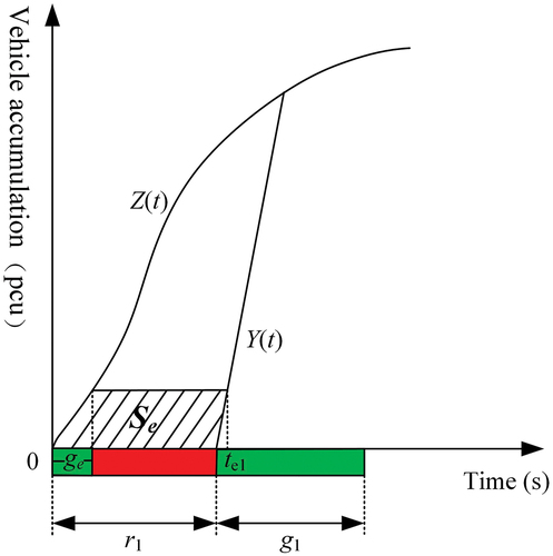
As shown in Figure 5, when the GE strategy is adopted, the formula for calculating the reduction in the delay of social vehicles in bus priority phase lane β is

(31) $\mathrm{\Delta }{D}_{\mathrm{c}1,\hspace{0.17em}\beta }={\int }_0^{g_{\mathrm{e}}}Z\left(t\right)dt+\left(t_{\mathrm{e}1}-g_{\mathrm{e}}\right)\cdot Z\left(g_{\mathrm{e}}\right)-{\int }_{r_1}^{t_{\mathrm{e}1}}Y\left(t\right)dt$(31)

When the GE strategy is adopted, the formula for calculating the reduction in the total passenger-delay for cars in the bus priority phase is

(32) $\mathrm{\Delta }{D}_{\mathrm{c}\mathrm{a}{\mathrm{r}}_1}=p_{\mathrm{c}}\cdot \sum _{\beta =1}^e\mathrm{\Delta }{D}_{\mathrm{c}1,\hspace{0.17em}\beta }$(32)

where e represents the number of lanes in the bus priority phase, and p_c represents the average passenger capacity of pure electric and fuel cars.

Therefore, when the GE strategy is adopted, the calculation formula for the total passenger-delay reduction of the bus priority phase is

(33) $\mathrm{\Delta }{D}_{\mathrm{p}1}=\mathrm{\Delta }{D}_{\mathrm{b}1}^2+\mathrm{\Delta }{D}_{\mathrm{b}2}^2+\mathrm{\Delta }{D}_{\mathrm{c}\mathrm{a}{\mathrm{r}}_1}$(33)

(b) Increased delay in non-bus priority phase

After the GE strategy is adopted, the green-light time of the non-bus priority phase is “occupied” by the bus priority phase, resulting in an increased delay of social vehicles in the non-priority phase, as shown in Figure 6.

Figure 6. Increased delay of social vehicles in the non-bus priority phase with GE strategy.

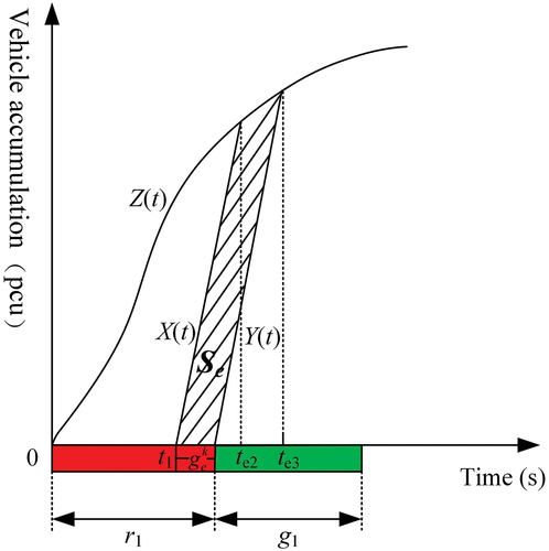
As shown in Figure 6, when the GE strategy is adopted, the formula for calculating the increase in the delay of social vehicles in the non-bus priority phase k lane j is

(34) $\mathrm{\Delta }{D}_{\mathrm{c}2,\hspace{0.17em}j}^k={\int }_0^{t_{\mathrm{e}3}}Z\left(t\right)dt-{\int }_{t_1+g_{\mathrm{e}}^k}^{t_{\mathrm{e}3}}Y\left(t\right)dt-{\int }_0^{t_{\mathrm{e}2}}Z\left(t\right)dt+{\int }_{t_1}^{t_{\mathrm{e}2}}X\left(t\right)dt$(34)

Let the function of the vehicle dissipation curve Y (t) be expressed as

(35) $Y\left(t\right)=at+b$(35)

Then, X (t) is expressed as

(36) $X\left(t\right)=Y\left(t\right)+a\cdot g_{\mathrm{e}}^k$(36)

Therefore, when the GE strategy is adopted, the formula for calculating the total passenger-delay for social vehicles in the non-bus priority phase is

(37) $\mathrm{\Delta }{D}_{\mathrm{c}\mathrm{a}{\mathrm{r}}_2}=p_{\mathrm{c}}\cdot \sum _{k=1}^n\sum _{j=1}^m\mathrm{\Delta }{D}_{c2,\hspace{0.17em}j}^k$(37)

In summary, the formula for calculating the total passenger-delay reduction under the GE strategy is

(38) $\mathrm{\Delta }{D}_2=\mathrm{\Delta }{D}_{\mathrm{p}1}-\mathrm{\Delta }{D}_{\mathrm{c}\mathrm{a}{\mathrm{r}}_2}$(38)

Therefore, when the combination strategy of guidance acceleration and GE is adopted, the calculation formula for the reduced total passenger-delay is

(39) $\mathrm{\Delta }{D}^{\prime }=\mathrm{\Delta }{D}_1+\mathrm{\Delta }{D}_2$(39)

(3) Guidance deceleration and RT

The delay caused by using the RT strategy at intersections includes the delay reduction in the bus priority phase and the delay increase in the non-bus priority phase (Bayrak and Guler 2020).

(1) Delay reduction of bus priority phase

After the RT strategy is adopted, the reduced delay of the bus at the intersection can be divided into stop-start and queuing delays. The calculation formula is

(40) $\left\{\begin{array}{c}\mathrm{\Delta }{D}_{\mathrm{b}1}^3=p_{\mathrm{b}1}\cdot \left[\frac{v_{\mathrm{b}1}^1}{2a_1}+\frac{v_{\mathrm{b}1}^1}{2a_2}+r_2\right]\\ \mathrm{\Delta }{D}_{\mathrm{b}2}^3=p_{\mathrm{b}2}\cdot \left[\frac{v_{\mathrm{b}2}^1}{2a_1}+\frac{v_{\mathrm{b}2}^1}{2a_2}+r_2\right]\end{array}\right.$(40)

where $\mathrm{\Delta }{D}_{\mathrm{b}1}^3$ and $\mathrm{\Delta }{D}_{\mathrm{b}2}^3$ represent the reduced delays of the pure electric and natural-gas buses, respectively, in the priority phase when the RT strategy is adopted.

The delay of social vehicles in the same priority phase as buses is also reduced by adopting the RT strategy, as shown in Figure 7.

Figure 7. Reduced delay of social vehicles in the bus priority phase with RT strategy.

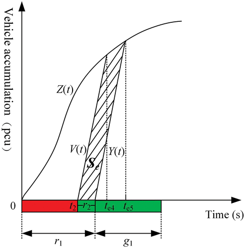
As shown in Figure 7, when the red truncation strategy is adopted, the delay reduction of social vehicles in bus priority phase lane β is given as

(41) $\mathrm{\Delta }{D}_{\mathrm{c}3,\beta }={\int }_0^{t_{\mathrm{e}5}}Z\left(t\right)dt-{\int }_{t_2+r_2}^{t_{\mathrm{e}5}}Y\left(t\right)dt-{\int }_0^{t_{\mathrm{e}4}}Z\left(t\right)dt+{\int }_{t_2}^{t_{\mathrm{e}4}}V\left(t\right)dt$(41)

Similarly, the function V (t) is expressed as

(42) $V\left(t\right)=Y\left(t\right)+a\cdot r_2$(42)

Therefore, when the RT strategy is adopted, the formula for calculating the reduced total passenger-delay of social vehicles in the bus priority phase is

(43) $\mathrm{\Delta }{D}_{\mathrm{c}\mathrm{a}{\mathrm{r}}_3}=p_{\mathrm{c}}\cdot \sum _{\beta =1}^e\mathrm{\Delta }{D}_{\mathrm{c}3,\beta }$(43)

Then, the formula for calculating the reduction in the total passenger-delay in the bus priority phase under the RT strategy is

(44) $\mathrm{\Delta }{D}_{\mathrm{p}2}=\mathrm{\Delta }{D}_{\mathrm{b}1}^3+\mathrm{\Delta }{D}_{\mathrm{b}2}^3+\mathrm{\Delta }{D}_{\mathrm{c}\mathrm{a}{\mathrm{r}}_3}$(44)

(b) Increased delay in non-bus priority phase

The green-light time of the non-bus priority phase is “occupied” when the RT strategy is adopted, which increases the delay of social vehicles in the non-bus priority phase, as shown in Figure 8.

Figure 8. Increased delay of social vehicles in the non-bus priority phase with RT strategy.

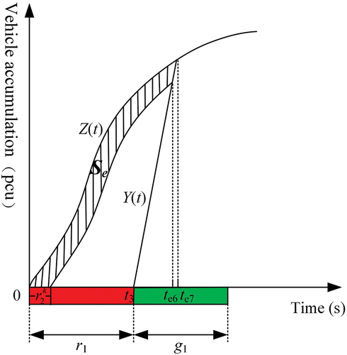
As shown in Figure 8, when the RT strategy is adopted, the formula for calculating the increased delay of social vehicles in the non-bus priority phase k lane j is

(45) $\mathrm{\Delta }{D}_{\mathrm{c}4,\hspace{0.17em}j}^k={\int }_0^{t_{\mathrm{e}7}}Z\left(t\right)dt-{\int }_{r_2^k}^{t_{\mathrm{e}6}}Z\left(t-r_2^k\right)dt-{\int }_{t_{\mathrm{e}6}}^{t_{\mathrm{e}7}}Y\left(t\right)dt$(45)

Therefore, when the RT strategy is adopted, the formula for calculating the increased total passenger-delay of social vehicles in the non-bus priority phase is

(46) $\mathrm{\Delta }{D}_{\mathrm{c}\mathrm{a}{\mathrm{r}}_4}=p_{\mathrm{c}}\cdot \sum _{k=1}^n\sum _{j=1}^m\mathrm{\Delta }{D}_{\mathrm{c}4,\hspace{0.17em}j}^k$(46)

In summary, when the RT strategy is adopted, the formula for calculating the reduced total passenger-delay is

(47) $\mathrm{\Delta }{D}_3=\mathrm{\Delta }{D}_{\mathrm{p}2}-\mathrm{\Delta }{D}_{\mathrm{c}\mathrm{a}{\mathrm{r}}_4}$(47)

Then, when the combination strategy of guidance deceleration and RT is adopted, the formula for calculating the reduced total passenger-delay is

(48) $\mathrm{\Delta }{D}^{{ }^{\prime \prime }}=\mathrm{\Delta }{D}_1+\mathrm{\Delta }{D}_3$(48)

When the speed-guidance control strategy is adopted, the unit energy consumption differs for different guidance speeds. The reduced total passenger-delay may not be optimal under optimal carbon -emission reductions. Using a combination optimization approach, with the optimal total passenger-delay reduction under BPC as the objective function and the guidance speed and compressed green-light time of the non-bus priority phase as the decision variables, the lower-level optimization model is constructed as follows:

$\begin{array}{rl}& max\mathrm{\Delta }D=\left\{\begin{array}{c}\mathrm{\Delta }{D}_1,\mathrm{g}\mathrm{u}\mathrm{i}\mathrm{d}\mathrm{a}\mathrm{n}\mathrm{c}\mathrm{e}\mathrm{a}\mathrm{c}\mathrm{c}\mathrm{e}\mathrm{l}\mathrm{e}\mathrm{r}\mathrm{a}\mathrm{t}\mathrm{i}\mathrm{o}\mathrm{n}\\ \mathrm{\Delta }{D}_1+\mathrm{\Delta }{D}_2,\mathrm{g}\mathrm{u}\mathrm{i}\mathrm{d}\mathrm{a}\mathrm{n}\mathrm{c}\mathrm{e}\mathrm{a}\mathrm{c}\mathrm{c}\mathrm{e}\mathrm{l}\mathrm{e}\mathrm{r}\mathrm{a}\mathrm{t}\mathrm{i}\mathrm{o}\mathrm{n}\mathrm{a}\mathrm{n}\mathrm{d}GE\\ \mathrm{\Delta }{D}_1+\mathrm{\Delta }{D}_3,\mathrm{g}\mathrm{u}\mathrm{i}\mathrm{d}\mathrm{a}\mathrm{n}\mathrm{c}\mathrm{e}\mathrm{d}\mathrm{e}\mathrm{c}\mathrm{e}\mathrm{l}\mathrm{e}\mathrm{r}\mathrm{a}\mathrm{t}\mathrm{i}\mathrm{o}\mathrm{n}\mathrm{a}\mathrm{n}\mathrm{d}RT\end{array}\right.\\ & s.t.\left\{\begin{array}{c}{v}_{min}\le v_{b1}^1\le v_{max}\\ v_{min}\le v_{b2}^1\le v_{max}\\ g_e=\sum _{k=1}^n{g}_e^k\\ r_2=\sum _{k=1}^n{r}_2^k\\ g_1^k-g_e^k\ge g_{min}^k\\ g_e\le g_{e\mathrm{\_}max}\hspace{0.17em}\\ r_2\le r_{2\mathrm{\_}max}\end{array}\right.\end{array}(49)$

Model solving algorithm design

In the above bi-level optimization model, the lower-level model is optimized under the decision variables of the upper-level model according to its own constraints and objective function, and then the optimization solution is fed back to the upper-level model to obtain the overall optimal solution in the feasible region. Considering that the objective functions of the upper- and lower-level models are polynomial, the Gauss – Seidel iteration idea can be used for reference, and diagonalization technology can be used to optimize the solution (Li and Zhang 2021; Montoya et al. 2019). The specific solution steps are as follows.

Step (1): Fix the decision variables $v_{\mathrm{b}1}^1$, $v_{\mathrm{b}2}^1$, $g_{\mathrm{e}}^k$, and $r_2^k$ (k = 1, … , n) of the upper-level model and consider the lower-level objective function as f (t₁, … , t_z), where z represents the number of decision variables, and t₁, … , t_z represent $v_{\mathrm{b}1}^1$, … , $r_2^k$, respectively. Let the lower-level variable be $T_p$ = ($t_1^p$, $t_2^p$, … , $t_j^p$, … , $t_z^p$) after the p^th outer-loop iteration. Initialize the element number j in $T_p$ as 1, the number of outer-loop iterations p as 0, and the value of the objective function as 0. The initial solution $T_0$ = ($t_1^0$, $t_2^0$, … , $t_j^0$, … , $t_z^0$) is generated randomly according to the constraints of the lower variables.

Step (2): Define $T^{t_{j^{-}}}$ as the set of variables excluding $t_j$, i.e., $T^{j^{-}}$= (t₁, t₂, … , $t_j$, … , t_z). Assign $T_{p+1}$ = $T_p$ and perform diagonalized iterations of the decision variables of the lower-level objective function.

Step (3): If $t_j$∈{$v_{\mathrm{b}1}^1$, $v_{\mathrm{b}2}^1$, $g_{\mathrm{e}}^k$, $r_2^k$}, j = j + 1, temporarily fix $T^{t_{j^{-}}}$ to obtain f($t_j,T^{t_{j^{-}}}$), where $t_j$∈($t_{\mathrm{m}\mathrm{i}\mathrm{n}j}$,$\hspace{0.17em}{t}_{\mathrm{m}\mathrm{a}\mathrm{x}j}$) and $t_{\mathrm{m}\mathrm{i}\mathrm{n}j}$ and $t_{\mathrm{m}\mathrm{a}\mathrm{x}j}$ are the upper and lower bounds of $t_j$, respectively.

Step (4): Compute the value of $t_j$ that satisfies $\frac{\mathrm{\partial }f\left(t_j,T^{t_{j^{-}}}\right)}{\mathrm{\partial }{t}_j}$ = 0, which is denoted as $\overline{t_j}$.

Step (5): If $\overline{t_j}$∈($t_{\mathrm{m}\mathrm{i}\mathrm{n}j}$,$\hspace{0.17em}{t}_{\mathrm{m}\mathrm{a}\mathrm{x}j}$), compute $max\left\{f\left(t_{minj},\hspace{0.17em}{T}^{t_{min{j}^{-}}}\right),\hspace{0.17em}f\left(\overline{t_j},\hspace{0.17em}{T}^{{\bar{t}}_{j^{-}}}\right),\hspace{0.17em}f\left(t_{maxj},\hspace{0.17em}{T}^{t_{max{j}^{-}}}\right)\right\}$; otherwise, compute $max\left\{f\left(t_{minj},\hspace{0.17em}{\mathrm{T}}^{t_{min{j}^{-}}}\right),\hspace{0.17em}f\left(t_{maxj},\text{break}\hspace{0.17em}{\mathrm{T}}^{t_{max{j}^{-}}}\right)\right\}$, and assign the corresponding $t_j$ to $t_j^{k+1}$, j = j + 1.

Step (6): The small-loop termination criterion is as follows. If j > z, p = p + 1; execute Step (7). Otherwise, return to Step (3).

Step (7): Optimize the decision variables in the upper-level model; temporarily fix the decision variables in the lower-level model; iterate diagonally on the decision variables in the upper-level model; update $v_{\mathrm{b}1}^1$, $v_{\mathrm{b}2}^1$, $g_{\mathrm{e}}^k$, and $r_2^k$; and obtain $T^p$.

Step (8): The convergence criterion of a large cycle is as follows. If $|f\left(T^{p+1}\right)-f\left(T^p\right)|$ satisfies the convergence accuracy, stop the iteration process. Otherwise, j = 1; proceed to Step (2).

Example analysis

Experimental design

In this study, we considered a four-phase intersection at the peak hour of a working day in Chongqing as the research object of BPC, and the corresponding data obtained after an investigation and statistical analysis were as follows: the cycle length of the signal light was 90 s, the north – south straight phase was the bus priority phase, no yellow light time was set for each phase, and right-turning vehicles were not controlled by the signal. The green-light time of each phase is shown in Figure 9. The average passenger capacity of pure electric and natural-gas buses was 50 persons, and the braking acceleration and starting acceleration were 3.0 and 2.0 m·s⁻², respectively. The average passenger capacity of pure electric and fuel cars was 2.5 persons, and the braking acceleration and starting acceleration were 3.5 and 2.5 m·s⁻², respectively. According to the carbon-emission coefficient conversion of the fuel consumption structure of electric energy production in Chongqing (Tang, Liu, and Chen 2015), the carbon-emission factor of electric vehicles was 565 gCO₂/(kW·h), and the carbon-emission factors of natural-gas and fuel vehicles were 2.16 and 2.08 gCO₂/mL, respectively (Sinha and Chaturvedi 2018). The unit energy consumption of pure electric and natural-gas buses under deceleration was 0.0091 (kW·h)/s and 6.09 mL/s, respectively; the unit energy consumption under acceleration was 0.0388 (kW·h)/s and 26.32 mL/s, respectively; and the unit energy consumption during idling was 0.0185 (kW·h)/s and 12.57 mL/s, respectively. The unit energy consumption of pure electric and fuel cars was 0.0028 (kW·h)/s and 0.31 mL/s, respectively, under deceleration; 0.0119 (kW·h)/s and 1.34 mL/s, respectively, under acceleration; and 0.0057 (kW·h)/s and 0.64 mL/s, respectively, during idling. The initial speed of pure electric and natural-gas buses was 30 km/h, the initial speed of pure electric and fuel cars was 50 km/h, and the distance of the speed-guidance area was 150 m. The arrival rates of pure electric and fuel cars and the saturation flow rate of the intersection entrance are presented in Table 1.

Figure 9. Schematic of the four-phase signal control scheme.

Table 1. Social vehicle arrival rate at the intersection.

Direction of entrance	South entrance goes straight	Turn left at south entrance	North entrance goes straight	Turn left at north entrance	East entrance goes straight	Turn left at east entrance	West entrance goes straight	Turn left at west entrance
Arrival rate of pure electric cars (pcu/s)	0.04	0.04	0.05	0.04	0.05	0.05	0.06	0.04
Arrival rate of fuel cars (pcu/s)	0.26	0.15	0.25	0.15	0.22	0.20	0.24	0.20
Saturation flow rate (pcu/s)	1.30	0.41	1.30	0.41	1.02	0.72	1.02	0.72

Analysis of results

To calculate the delay variation of the bus priority phase and non-priority phase, the saturation flow rate at the intersection entrance was used as the vehicle dissipation function, and the least-squares fitting method was used to fit the vehicle accumulation function at the intersection entrance. The results are presented in Table 2.

Table 2. Fitting coefficients of the vehicle accumulation function at the intersection.

Direction of entrance	Polynomial basis functions	x^3	x^2	x	1
	Polynomial coefficient	b1	b2	b3	b0
South entrance	Go straight	−1.01E–04	1.47E–02	−1.66E–01	9.61E–01
	Turn left	−2.33E–05	3.05E–03	5.40E–02	−1.56E–01
North entrance	Go straight	−7.78E–05	1.15E–02	−4.52E–02	1.31E–01
	Turn left	−2.85E–05	4.36E–03	−1.29E–02	2.21E–01
East entrance	Go straight	−1.39E–05	2.04E–03	5.73E–02	1.50E–02
	Turn left	−1.158E–05	1.60E–03	1.96E–02	1.74E–01
West entrance	Go straight	−1.93E–05	2.73E–03	4.10E–02	2.85E–01
	Turn left	−1.54E–05	2.07E–03	2.16E–02	9.63E–02

(1) Guidance acceleration

According to the above data, when the bus arrived at the speed-guidance area and the remaining green-light time of the bus priority phase is 15 s, if the corresponding control strategy is not adopted, the bus cannot pass through the intersection during the remaining green-light time. In contrast, if the guidance acceleration strategy is adopted, the bus can pass through the intersection without stopping, and the carbon emissions and total passenger-delay are reduced. The reductions in the carbon emissions and total passenger-delay at different guidance speeds are presented in Figure 10.

Figure 10. Changes in the carbon emissions and total passenger-delay under the guidance acceleration strategy.

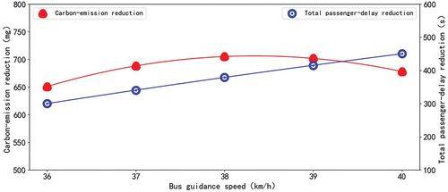
As shown in Figure 10, with an increase in the guidance speed, the carbon-emission reductions first increased and then decreased. Because the delay reduction only increased with an increase in speed, it exhibited a gradually increasing trend. When the guidance speed was 38 km/h, the carbon-emission reductions were maximized (705.12 mg), and the reduction rate was 12.67%. The total delay was 378.94 s, and the reduction rate was 21.05%. Therefore, when the remaining green-light time is long, the guidance acceleration strategy has a significant impact on reducing the carbon emissions and total passenger delay.

(2) Guidance acceleration and GE

If the bus arrives at the speed-guidance area and the remaining green-light time at the intersection is only 10 s, it is impossible for the bus to pass through the intersection without stopping using only the guidance acceleration strategy. In this case, it is necessary to use a combined strategy of guidance acceleration and GE. The reduced carbon emissions and total passenger delay under different guidance speed and green-light extension time are shown in Figure 11, and the change in the average stopping times for each phase is shown in Figure 12.

Figure 11. Changes in the carbon emissions and total passenger-delay under guidance acceleration and GE strategy.

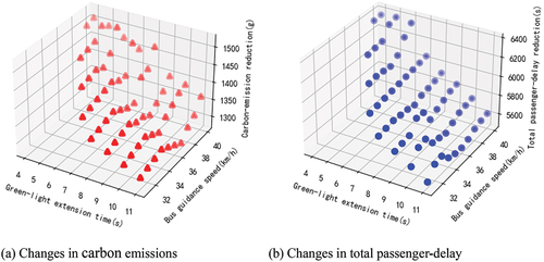
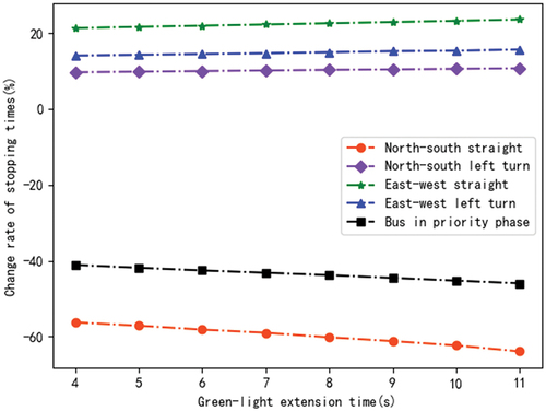
Figure 12. Optimization results for the average stopping times with the GE strategy.

As shown in Figure 11, the combination strategy of guidance acceleration and GE significantly reduced the carbon emissions and total passenger-delay generated by the bus in the upstream section of the intersection and intersection control area. The calculations indicated that when the guidance speed was 39 km/h and the green-light extension time was 6 s, the largest carbon-emission reductions were 1528.03 g, with a reduction rate of 27.49%, and the total passenger-delay reduction was 6254.31 s, with a reduction rate of 38.62%.

As shown in Figure 12, as the green-light extension time increased, the average stopping times in the bus priority phase decreased, and the average stopping times in the non-bus priority phase increased. When the guidance speed and GE were optimal, that is, when the guidance speed was 39 km/h and the green-light extension time was 6 s, the average stopping times in the north – south straight phase decreased by 58.18%. The average stopping times in the north – south left turn, east – west straight, and east – west left turn phases increased by 10.41%, 21.94%, and 14.47%, respectively, and the average stopping times of buses in the priority phase decreased by 42.58%.

(3) Guidance deceleration and RT

If the bus arrives early, that is, when it arrives at the intersection in the red-light state, and the remaining red-light time is 5 s, a combination strategy of guidance deceleration and RT is adopted to allow it to pass through the intersection without stopping. The reduced carbon emissions and total passenger-delay with different guidance speed and red-light shortening times are shown in Figure 13, and the change in the average stopping times for each phase is shown in Figure 14.

Figure 13. Changes in the carbon emissions and total passenger-delay with guidance deceleration and RT strategy.

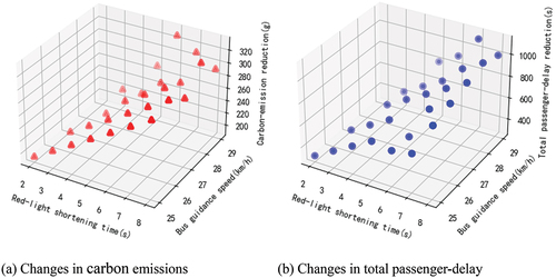
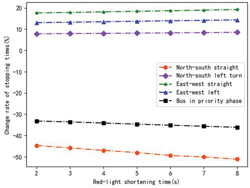
Figure 14. Optimization results for the average stopping times with the RT strategy.

As shown in Figure 13, the combination strategy of guidance deceleration and RT significantly reduced the carbon emissions and total passenger-delay generated by the bus during the driving process and increased the overall capacity at the intersection when the early arrival time of the bus is short. The calculations indicated that when the guidance speed was 29 km/h and the red-light shortening time was 6 s, the largest carbon-emission reductions were 312.20 g, with a reduction rate of 22.18%, and the reduction in the total passenger-delay was 914.61 s, with a reduction rate of 33.52%.

As shown in Figure 14, as the green-light extension time increased, the average stopping times in the bus priority phase decreased, and the average stopping times in the non-bus priority phase increased. When the guidance speed and RT were optimal, that is, when the guidance speed was 29 km/h and the red-light shortening time was 6 s, the average stopping times in the north – south straight phase decreased by 49.39%. The average stopping times in the north – south left turn, east-west straight, and east-west left turn phases increased by 8.27%, 18.68%, and 13.96%, respectively, and the average stopping times of buses in the priority phase increased by 35.15%.

Sensitivity analysis

(1) Speed guidance area distance

To verify the impact of the distance of the speed-guidance area on the traffic carbon emissions, we assumed that the guidance speed was 35 km/h and all other conditions remained unchanged; the distance of the speed-guidance area was varied in the range of 100–150 m, when the remaining green-light time and red-light time were 5 and 18 s, respectively. The relationship between the change in carbon emissions and the distance of the speed-guidance area when the GE and RT strategies were adopted is shown in Figure 15.

Figure 15. Sensitivity analysis of the distance of the speed-guidance area with different priority strategies.

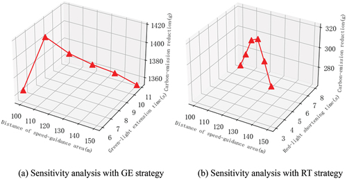
As shown in Figure 15, when the GE or RT strategy was adopted, with an increase in the distance of the speed-guidance area, the carbon-emission reductions first increased and then decreased. For Figure 15(a), when the distance of the speed-guidance area was>120 m, the change range of the carbon-emission reductions were relatively flat. For Figure 15(b), when the distance of the speed-guidance area was>130 m, the change range of the carbon-emission reductions were relatively flat. Therefore, it can be concluded that the model developed in this study is more suitable for scenarios where the distance of the speed-guidance area is >130 m.

(2) Car arrival rate in bus priority phase

Assuming that all other conditions are kept constant, the speed of bus arriving at the priority phase of the intersection is 40 km/h. Under the condition that the ratio of the arrival rate of pure electric and fuel cars in the bus priority phase remains unchanged, the value of the arrival rate is changed year-on-year to study its impact on the overall carbon emission reduction of the intersection under the strategy of green extension or red truncation, and the results are shown in Figure 16.

Figure 16. Sensitivity analysis of the car arrival rate in the bus priority phase.

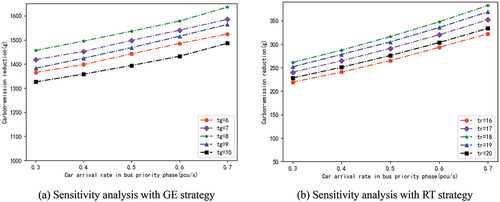
As shown in Figure 16, under the green extension and red truncation strategies, when the car arrival rate of the bus priority phase varies in the range of 0.3–0.7 pcu/s, the reduced carbon emissions within the intersection also shows a gradual upward trend, but the change range is relatively flat with the increase of the car arrival rate, and the change trends of the model optimization results are similar with the difference of the remaining green-light times ($t_{\mathrm{g}}$) and red-light times ($t_{\mathrm{r}}$). Therefore, it can be explained that the model has good stability.

Conclusion

Under speed guidance and BSPC strategies, we analyzed the changes in the carbon emissions and total passenger-delay for bus and social vehicles of different fuel types in the upstream section of the intersection and intersection control area. We used a combination optimization approach to develop a bi-level optimization model for BPC. The following conclusions are drawn.

1. The effects of main parameters, such as the delay, stopping times, and speed, on the traffic carbon emissions were analyzed. Vehicle delay was divided into acceleration, deceleration, and idle delays. Considering the impact of multiple stops on traffic carbon emissions, according to the different carbon emissions per unit mileage at different speeds, a calculation method for traffic carbon emissions under different parameters was developed.

2. Three control methods were studied: guidance acceleration, guidance acceleration and GE, and guidance deceleration and RT. On the basis of the kinematics formula and geometric analysis method, a calculation method for the carbon emissions and delay in the bus priority phase and non-priority phase was developed.

3. With the optimal carbon-emission reductions as the upper-level objective and the optimal delay reduction as the lower-level objective, a bi-level optimization model for BPC was developed, and the results of an example analysis indicated that the model can effectively reduce the carbon emissions of vehicles and total passenger-delay and achieve bus priority with the optimal overall traffic efficiency.

We have only studied part of the BPC and suggest that further research can be focused on the following aspects in the future.

1. Because the values of $L_b$ in the model developed in this study are subjective, the effect of the randomness of the parameter value in the bi-level optimization model for the BPC can be considered in a subsequent study to improve the applicability of the model.

2. This study was based on the assumption that buses are driving in bus lanes. Subsequent research can focus on BPC under non-bus lane conditions.

Disclosure statement

No potential conflict of interest was reported by the authors.

Data availability statement

The data that support the findings of this study are available on request from the corresponding author. The data are not publicly available due to their containing information that could compromise the privacy of research participants.

Additional information

Funding

This work was supported by the Chongqing Social Science Planning Project (Grant No. 2021NDYB035), Sichuan Science and Technology Program (Grant No. 2022YFG0132) and the Chongqing Postgraduate Joint Training Base Project (Chongqing Jiaotong University-Chongqing YouLiang Science & Technology Co., Ltd Joint Training Base for Postgraduates in Transportation) (Grant No. JDLHPYJD2019007).

Notes on contributors

Xinghua Hu

Xinghua Hu is a professor at Chongqing Jiaotong University who is engaged in the research of transportation carbon emission big data analysis and green low carbon policy.

Xinghui Chen

Xinghui Chen is a master's student studying regional and urban transportation system planning at Chongqing Jiaotong University.

Jianpu Guo

Jianpu Guo is an associate researcher at the Department of Science and Technology Statistics and Innovation Development in Chongqing.

Gao Dai

Gao Dai is a senior engineer in the Technology R & D Department of Chongqing Ulit Science and Technology Co. Ltd.

Bing Long

Bing Long is a senior engineer at the Institute of Traffic Engineering, Chongqing Transport Planning Institute.

Xiaoyan Chen

Xiaoyan Chen is a senior engineer engaged in research on energy conservation, emission reduction and environmental protection in transportation at the Institute of Strategic Planning, Institute of Transportation Development Strategy and Planning of Sichuan Province.

References

- Anderson, P., and C.F. Daganzo. 2020. Effect of transit signal priority on bus service reliability. Transp. Res. Part B 132:2–14. doi:10.1016/j.trb.2019.01.016.
- Anser, M.K., D.I. Godil, M.A. Khan, A.A. Nassani, K. Zaman, and M.M. Q. Abro. 2021. The impact of coal combustion, nitrous oxide emissions, and traffic emissions on COVID-19 cases: A Markov-switching approach. Environ. Sci. Pollut. Res. 28 (45):64882–91. doi:10.1007/s11356-021-15494-x.
- Bayrak, M., and S.I. Guler. 2020. Determining optimum transit signal priority implementation locations on a network. Transp. Res. Rec. 2674 (10):387–400. doi:10.1177/0361198120934792.
- Bie, Y., X. Xiong, Y. Yan, and X. Qu. 2020. Dynamic headway control for high‐frequency bus line based on speed guidance and intersection signal adjustment. Comput.-Aided Civ. Infrastruct. Eng. 35 (1):4–25. doi:10.1111/mice.12446.
- Ceylan, H., and M.G. Bell. 2020. Traffic signal timing optimisation based on genetic algorithm approach, including drivers’ routing. Transp. Res. Part B 38 (4):329–42. doi:10.1016/S0191-2615(03)00015-8.
- Chłopek, Z., J. Lasocki, P. Wójcik, and A.J. Badyda. 2018. Experimental investigation and comparison of energy consumption of electric and conventional vehicles due to the driving pattern. Int. J. Green Energy 15 (13):773–79. doi:10.1080/15435075.2018.1529571.
- Ghafari, A., and M. Akbarzadeh. 2021. Evaluation of the impacts of unconditional active transit signal priority in VISSIM, case study: A corridor in Isfahan. Amirkabir. J. Civ. Eng. 53 (1):201–12.
- Ghosh, T., K. Bhattacharyya, and B. Maitra. 2022. Traffic micro-simulation-based evaluation of bus priority with queue jump lane on an urban corridor with heterogeneous traffic operations. Transp. Res. Rec. 20 (2):15–41.
- Girijan, A., L.D. Vanajakshi, and B.R. Chilukuri. 2021. Dynamic thresholds identification for green extension and red truncation strategies for bus priority. IEEE Access 9:64291–305. doi:10.1109/ACCESS.2021.3074361.
- Hallmark, S.L., I. Fomunung, R. Guensler, and W. Bachman. 2020. Assessing impacts of improved signal timing as a transportation control measure using an activity-specific modeling approach. Transp. Res. Rec. 1738 (1):49–55. doi:10.3141/1738-06.
- Hasan, M.M., N. Avramis, M. Ranta, A. Saez-de-Ibarra, M. El Baghdadi, and O. Hegazy. 2021. Multi-objective energy management and charging strategy for electric bus fleets in cities using various ECO strategies. Sustainability 13 (14):7865. doi:10.3390/su13147865.
- Hu, X., B. Long, and X. Zhu. 2016. Timing optimization for bus priority signalized intersection considering green loss equilibrium. J. Highway Transp. Res. Dev. 33 (02):96–104. in Chinese.
- Hu, X., Y. Xu, J. Guo, T. Zhang, Y. Bi, W. Liu, and X. Zhou. 2022. A complete information interaction-based bus passenger flow control model for epidemic spread prevention. Sustainability 14 (13):8032. doi:10.3390/su14138032.
- Hussain, Z., M.K. Khan, and W.A. Shaheen. 2022. Effect of economic development, income inequality, transportation, and environmental expenditures on transport emissions: Evidence from OECD countries. Environ. Sci. Pollut. Res 29 (37):56642–57. doi:10.1007/s11356-022-19580-6.
- Karekla, X., R. Fernandez, and N. Tyler. 2018. Environmental effect of bus priority measures applied on a road network in Santiago, Chile. Transp. Res. Rec. 2672 (8):135–42. doi:10.1177/0361198118784134.
- Kim, H., Y. Cheng, and G.L. Chang. 2018. Variable signal progression bands for transit vehicles under dwell time uncertainty and traffic queues. IEEE Trans. Intell. Transp. Syst. 20 (1):109–22. doi:10.1109/TITS.2018.2801567.
- Koehler, L.A., L.O. Seman, W. Kraus, and E. Camponogara. 2018. Real-time integrated holding and priority control strategy for transit systems. IEEE Trans. Intell. Transp. Syst. 20 (9):3459–69. doi:10.1109/TITS.2018.2876868.
- Kwak, J., B. Park, and J. Lee. 2019. Evaluating the impacts of urban corridor traffic signal optimization on vehicle emissions and fuel consumption. Transp. Plann. Technol. 35 (2):145–60. doi:10.1080/03081060.2011.651877.
- Li, H., and Y. Zhang. 2021. A Greedy Gauss-Seidel method for solving the large linear least squares problem. J. Tongji Univ. (Nat. Sci.) 49 (11):1514–21. in Chinese.
- Montoya, O.D., V. M. Garrido, W. Gil-González, and L.F. Grisales-Noreña. 2019. Power flow analysis in DC grids: Two alternative numerical methods. IEEE Trans. Circuits Syst. II Express Briefs 66 (11):1865–69. doi:10.1109/TCSII.2019.2891640.
- Ou, S., C. Yu, and W. Wa. 2022. Connected bus real-time priority control considering arterial signal coordination. J. Tongji Univ. (Nat. Sci.) 50 (3):339–50. in Chinese.
- Parr, S.A., and E. Kaisar. 2021. Critical intersection signal optimization during urban evacuation utilizing dynamic programming. J. Transp. Saf. Secur. 3 (1):59–76. doi:10.1080/19439962.2011.532297.
- Seman, L.O., L.A. Koehler, E. Camponogara, and W. Kraus Jr. 2020. Integrated headway and bus priority control in transit corridors with bidirectional lane segments. Transp. Res. Part C 111:114–34. doi:10.1016/j.trc.2019.12.001.
- Sinha, R.K., and N.D. Chaturvedi. 2018. A graphical dual objective approach for minimizing energy consumption and carbon emission in production planning. J. Clean. Prod. 171:312–21. doi:10.1016/j.jclepro.2017.09.272.
- Tang, S., X. Liu, and Z. Chen. 2015. State discriminant and queue length estimation of an intersection based on video data. Road Traffic Saf. 15 (1):58–64.
- Thodi, B.T., B.R. Chilukuri, and L. Vanajakshi. 2022. An analytical approach to real-time bus signal priority system for isolated intersections. J. Intell. Transp. Syst. 26 (2):145–67. doi:10.1080/15472450.2020.1797504.
- Wahlstedt, J. 2011. Impacts of bus priority in coordinated traffic signals. Procedia-Social Behav. Sci. 16:578–87. doi:10.1016/j.sbspro.2011.04.478.
- Wunderlich, R., C. Liu, I. Elhanany, and T. Urbanik. 2020. A novel signal-scheduling algorithm with quality-of-service provisioning for an isolated intersection. IEEE Trans. Intell. Transp. Syst. 9 (3):536–47. doi:10.1109/TITS.2008.928266.