Local, forest stand and landscape-scale correlates of plant communities in isolated coastal forest reserves

Abstract

In mixed oak stands situated within two isolated forest reserves in NE Italy, we investigated how plant communities are modulated by local conditions, forest structure and landscape attributes. Species richness and functional dispersion increased towards canals, whereas soil salinity, canopy density or landscape heterogeneity were less relevant. Mean nutrient indicator values increased near canals and with higher proportions of agriculture around. Functional dispersion decreased at wet, nutrient rich sites. Also, the proportion of salt tolerant species increased towards canals, but was unrelated to measures of soil salinity. At sites with more modified landscapes around, widely distributed species were more prevalent, at cost of plants with restricted distributional ranges. Hence, biotic homogenization is fostered inside the reserves through landscape modification in their surroundings. In contrast to species richness, composition turned out to be markedly modulated by environmental variation, with local site factors, forest stand structure and landscape attributes contributing to roughly the same extent. Conservation practices should therefore not only focus on managing local conditions, but also take landscape structure into account. For coastal forests, dry and open, nutrient poor sites are of special conservation concern, which are believed to most closely resemble the original diverse vegetation of these Mediterranean habitats.

Keywords:

• Mediterranean forests
• species composition
• vegetation change
• biotic homogenization
• landscape-scale influence
• plant diversity
• conservation management
• nutrient spill-over

Introduction

The Mediterranean basin is one of the Earth’s biodiversity hotspots and – as such – home of about 25,000 native plant species (Myers et al. 2000; Cuttelod et al. 2009). Of these, about 50% are endemic to the region (Cowling et al. 1996). The evolution of today’s Mediterranean landscapes is strongly linked to millennia of human land-use, which historically contributed to the diverse and heterogeneous habitats (Blondel 2006). However, over the past decades accelerated land-use change, either through abandonment or through intensification, render Mediterranean habitats one of the globally most endangered areas facing biodiversity loss (Lavergne et al. 2005) and landscape homogenization (Geri et al. 2010). While inland, forest areas are increasing at the cost of open landscapes, coastal transformation led to the disappearance of most forest sites because of human population growth and urbanization, mass tourism and agricultural intensification (Falcucci et al. 2007). Remnant forest patches are often small sized, fragmented habitats which are highly isolated from another as they are surrounded by anthropogenically modified land (Teixido et al. 2010). Setting aside these areas from land-use as nature reserves forms an important part of conservation strategies to mitigate biodiversity loss (Araújo et al. 2007; Doxa et al. 2017). However, there are still environmental variables influencing the plant communities in isolated reserves. These factors can principally be distinguished into three groups:

• Primarily, natural variation in topography, local edaphic and hydrological conditions determines which plants from the regional species pool can populate an area, thereby forming the “potential natural vegetation” (Molina-Venegas et al. 2016).

• Second, factors associated with land-use history usually have left their imprint, for example, with regard to tree species composition, tree density and age structure of stands in case of forested sites (Sabatini et al. 2014; Burrascano et al. 2018).

• Finally, local ecological conditions may be altered by pressures that arise from the landscape around the reserve, for example, soil salinization (Mollema et al. 2013), spill-over of pollutants and fertilizers (Bussotti and Gerosa 2002; van Dobben and de Vries 2017), or increasing drought stress in the course of climate change (Liu et al. 2018; Peñuelas et al. 2018; Tsiafouli et al. 2018). Landscape-scale drivers of biota inside reserves also include edge effects (Wuyts et al. 2013), reduced habitat size or the extent of fragmentation and isolation of reserves (Rosati et al. 2010; Malavasi et al. 2016; Luzuriaga et al. 2018).

So, human activities can alter plant communities through past and present land-use intensity and management within reserves as well as through landscape-scale effects acting from the outside. As a consequence, functional homogenization, declining species diversity or the invasion of alien species can be observed in many conservation areas (Clavel et al. 2011; Malavasi et al. 2016; Bazzichetto et al. 2018).

In this study, using two protected coastal forest remnants in north-eastern Italy as an example, we address different aspects of local, (land-use history driven) forest and landscape characteristics in relation to their vegetation. By doing so, we aim to uncover the hierarchy of influences these factors have in shaping coastal forest plant communities. Especially, we focus on subtle differences in plant diversity, functional diversity and species composition within contiguous forest stands of broadly similar type. Two suites of anthropogenic factors are of special concern here. (1) The entire region is subject to increase in soil salinization, as a consequence of land subsidence (Mollema et al. 2013). (2) Directly adjacent to the two reserves there are large areas under intense agricultural use (Musolino et al. 2019) and highly urbanized areas (Lucialli et al. 2007). It is therefore likely that the surroundings of the two forest reserves have substantial influence on the local vegetation inside. In particular, we address the following questions:

• Can attributes of the local plant communities such as species richness, functional diversity or mean indicator values be related to any of the observed factors?

• Are landscape factors (e.g. the extent of modified land surrounding focal plots) driving plant communities from typical Mediterranean composition towards dominance by cosmopolitan species?

• Are local plant communities changing with the degree of soil salinization or is there a more general shift to salt tolerant plants all over the reserve areas?

• How much variation in plant community composition can be described at each of the three spatial scales (i.e. local, forest stand and landscape level)?

Methods

Study area

The coastline around Ravenna, NE Italy, has developed over centuries through sedimentation by the river Po and therefore is until today characterized by sandy soils and paleodunes (Antonellini et al. 2008). Our study sites were located inside two isolated relict forest reserves, Pineta san Vitale (hereafter PsV) and Pineta di Classe (hereafter PdC). Both reserves comprise an area of approximately 10 km², with PsV being elongated with 7 × 1.5 km² in shape and PdC having a more compact shape of about 5 × 2 km². Both forests have a long history of human land-use and management. Around 500 BC, when the first settlements of what today constitutes the city of Ravenna were built, large areas of mixed oak forests (mainly Quercus robur L. and Quercus pubescens Willd.) are believed to have covered the coastal areas (Andreatta 2010). About 400–500 AC historical notes for the first time mention “pine woods” in the area, which are believed to indicate the presence of Pinus sylvestris L. and Pinus nigra J.F. Arnold.

The area where PsV and PdC today are located is believed to have been developing in the tenth to fifteenth century through sedimentation (Buscaroli et al. 2011). Only during the tenth and eleventh century, when the forests were property of different abbeys (on which the recent names “san Vitale” and “Classe” are still based), stone pine trees (Pinus pinea L.) were introduced to the region. Stone pines were mainly planted on top of the paleodunes. In between, where soil conditions did not match the needs of pine trees, other forest types like mixed deciduous forest and riparian forest remained (Andreatta 2010). From the twelfth century onwards, Ravenna’s pine forests were used for pine nut harvest and wood production as well as for cattle grazing (Andreatta 2010). Until the end of the eighteenth century, these forests had reached their maximum expansion of about 6000 ha (Malfitano 2002). From 1796 onwards, many trees were cut down for ship building and for the sake of urban development. The forest areas got increasingly fragmented until only about 2000 ha, split up between the two areas PsV and PdC, were left (Malfitano 2002; Andreatta 2010). Pine nut production and other management practices were finally abandoned in 1988, when the “Parco regionale del Delta del Po” was established, protecting the two forests from further degradation (Enrica Burioli, pers. communication, http://demetra.regione.emilia-romagna.it, Assemblea legislativa della Regione Emilia‐Romagna 1988).

Being a part of the Parco regionale del Delta del Po, listed as UNESCO biosphere reserve (www.unesco.org, UNESCO 2015) and Natura 2000 sites and also partly flagged as important bird area (Bird Life International 2019), Ravenna’s coastal forests are today of high legal conservation status. After their planting during the Middle Ages, the ancient open pine woods developed due to natural succession and are today dominated by a mix of oak and pine forest (Wölfling et al. 2019), but also other vegetation types like grassland on sandy soils, reed vegetation and riparian forest sites can be found (Merloni and Piccoli 1999; Piccoli and Merloni 1999).

As the entire Po plain is today one of the most important areas for agricultural use in Italy (Musolino et al. 2019), conservation interests and intensive land-use often collide here. Also around PsV and PdC, highly modified landscapes including arable land, the industrial harbor of Ravenna and urban areas are a source of pressures on the nature reserves that are designated for conserving Mediterranean biodiversity.

Data collection

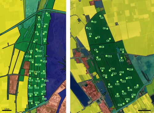
We partitioned each reserve into 30 grid cells (600 × 600 m²). In each grid cell, one sampling location was chosen by considering three criteria (Figure 1). (1) All sites should be situated inside the same vegetation type, viz. a mixture of oak and pine forest. This tree composition is closest to the former natural vegetation of the paleodunes. (2) Other habitat types like reed vegetation or open grassland should be at least 100 m away from the sampling location. (3) The sites had to be accessible from one of the numerous small pathways through the forests.

Figure 1. Schematic maps of the two study coastal pine forest reserves near Ravenna, NE Italy (left: PsV, right: PdC) and locations of the sampling sites (green dots, V1–30 in PsV, C1–30 in PdC). Landscape indicated by colors: forest (dark green), open habitats (light green), arable land (yellow), buildings (red), reed (light blue) and open water (dark blue). Modified using QGIS based on satellite images extracted from Google Maps.

Data collection took place from 2015 to 2017. Each year, 20 of the 60 locations were chosen randomly (10 in each reserve) and then sampled once between April and September. At each location soil samples, tree crown density and all plant species forming the herb, shrub and tree layer were analyzed.

The herb layer was sampled in April within five randomly chosen 1 × 1 m² plots per site. Each plot took approximately 0.5–1 h of time to register, resulting in about 2.5–5 h herb layer sampling per location. If necessary, flowering characteristics required for the identification of species were additionally checked in June. For the shrub layer five 5 × 5 m² plots per location were analyzed in September. All plants were identified to species level using different monographs (Aichele et al. 1998; Bassi 2004, Senghas and Seybold 2003) as well as the internet page www.actaplantarum.org (Acta Plantarum 2007). For further analyses, only plant species incidences per site were considered (Table S1).

For measurements of soil factors, 20 soil samples per location (five samples each in April, June, August and September) were taken. pH value and electric conductivity (EC) were measured using a Multiparameter Meter HI 9813 (Hanna Instruments). Out of these 20 measurements, a mean pH and a mean EC value (as proxy for soil salinity: Malicki and Walczak 1999) were calculated for each site. Further abiotic characteristics like humidity, local temperature, soil nutrients and light availability were inferred from Ellenberg’s indicator values of all plant species observed per site. Ellenberg indicator values have often proven as suitable proxies for the microclimatic and edaphic conditions they represent (Schaffers and Sýkora 2000). To this end, indicator values for all recorded plant species were extracted from Pignatti et al. (2005) and a non-weighted mean Ellenberg indicator value was calculated.

Composition and structure of the tree layer were recorded by doing 10 point-centered-quarter (PCQ) analyses per site in August following Mitchell (2010). PCQ as a distance-based method has some disadvantages compared to plot-based methods, like a larger sampling bias leading to over- or underestimations of the real community level forest density (Bryant et al. 2005). But as forest understory vegetation – especially shrub vegetation – in PsV and PdC is quite dense, no plot-based analyses were physically feasible. For the PCQ analyses, species identity and diameter at breast height (by only taking into account stems with a circumference bigger than 10 cm) of 40 trees (four trees per PCQ) were noted. Furthermore, the height of these trees was estimated by taking pictures of the whole tree together with a 1 m ruler as scale. The trees on the pictures were then measured using the program ImageJ 1.45s (Schneider et al. 2012). Out of these records, mean basal area and its standard deviation (as proxies for forest age and stand heterogeneity), mean tree height, forest density (as number of stems/ha) and forest cover (defined after Mitchell (2010) as stem density × mean basal area, in m²/ha) of conifer and deciduous trees were calculated. Tree crown density was measured at four random points using a manual densiometer (Forest densiometers, Robert E. Lemmon, Rapid City) four times each in April, June, August, September, resulting in 16 crown density measurements per location. Again, the mean value of these entered into subsequent statistical analyses.

Landscape composition and structure were analyzed using the software QGIS (QGIS Development Team 2018), based on satellite images from 2017 provided in Google Maps™. All calculations were done for a 1000 m buffer around each location, as larger landscape scales are believed to be more important for plant species composition than smaller ones (Amici et al. 2015). Specifically, from the satellite images the proportions (area) of forest, open grassland, reed vegetation, open water bodies, buildings, agricultural land and other structures (including roads and gardens) were recorded. Subsequently, forest, open grassland and reed vegetation were summarized as “near-natural areas”. As a corollary, buildings, agricultural land and other habitat structures were summarized as “modified land”. Furthermore, edge density in the landscape (expressed as length of all habitat edges per ha) and landscape diversity (expressed as Shannon diversity of fractions of area of the aforementioned elements, in its exponential version) were calculated (Schindler et al. 2015; Clément et al. 2017).

Finally, the nearest distance from each site to structural components of the landscape such as water canals and forest edges was measured using QGIS. All measured local, forest stand and landscape factors are shown in Table 1.

Table 1. List of all measured local, forest stand and landscape-level factors.

Local factors	Forest stand factors	Landscape factors
Soil pH	Mean tree basal area (cm²)	Distance to nearest forest edge (m)
Soil salinity (mg/l)	Standard deviation of tree basal area (cm²)	Distance to nearest canal (m)
Ellenberg indicator for light	Mean tree height (m)	Edge density (m/ha)
Ellenberg indicator for temperature	Forest density (number of stems/ha)	Landscape diversity (exponential Shannon)
Ellenberg indicator for humidity	Proportion of deciduous tree biomass (=deciduous biomass/complete biomass)	Natural areas (proportion)
Ellenberg indicator for nutrients	Crown density (proportion of visible sky)	Agricultural land (proportion)

Data analysis

For the calculation of distance based plant functional diversity, a matrix consisting of 46 traits was compiled. This matrix contained plant characteristics such as the life-form, presence of spines, resin or latex secretion, maximum plant height, root type, various flower and leaf attributes (like flowering time, leaf structure, phyllotaxy, pubescence, pollination syndrome, seed dispersion type and leaf phenology) as well as habitat and distribution characteristics (including Ellenberg indicator values, distributional range or salt tolerance) (Table S2). Information about plant traits was collated from monographs (Aichele et al. 1998; Senghas and Seybold 2003; Bassi 2004; Burnie 2007; Schönfelder and Schönfelder 2011) as well as from the internet page www.actaplantarum.org (Acta Plantarum 2007). Information about salt tolerance was gathered from Böhling (1995), Flückiger (2007), Ellenberg and Leuschner (2010) and the internet page https://www.infoflora.ch (Infoflora 2004). For analysis, we scored all plant species known to grow naturally on salt-influenced soils or to tolerate salt under urban conditions as “salt-tolerant”. We further scored plant species according to their natural distributions into Mediterranean and widely distributed species. Functional diversity calculations were done in the R environment (Pinheiro et al. 2018) using the packages “vegan” (Oksanen et al. 2018) and “FD” (Laliberté and Legendre 2010; Laliberté et al. 2014). We used functional dispersion (FDis) as suggested by Laliberté and Legendre (2010) as this functional diversity index is not dependent on species richness per se (like, e.g., functional richness) and can also deal with incidence based species data, where it represents the unweighted mean distance to the centroid (viz. the dispersion of species in trait space) (Laliberté and Legendre 2010). For the hierarchical clustering tree of functional traits, the “hclust” function based on Gower dissimilarity and the Ward.D2 method was used. Functional dispersion analysis was done with the “dbFD” function, using the trait matrix and the incidence table of all observed vascular plants (herbs, shrubs and trees together).

To compare plant gamma diversity between the two study areas, total plant species richness for each reserve was estimated by doing a sample based extrapolation after Chao et al. (2016) using the program iNEXT. Indicator plant species for each of the two reserves were extracted using the “indval” function with the “labdsv” package (Roberts 2016). Differences between local species richness and local FDis of the PsV and PdC locations were tested using student’s t-test with the basic “stats” package in R.

All environmental factors available for each site (Table 1) were checked for normality and transformed if necessary. Proportions were logit transformed (Warton and Hui 2011). To assess how averaged local plant indicator values for humidity, temperature, light and nutrients are related to local, forest stand and landscape factors, linear mixed effects models were constructed, using the package “nlme” (Pinheiro et al. 2018). Reserve identity (PsV or PdC) was included as random factor.

Subsequently for further multivariate analysis, all environmental factors were z-transformed to a mean of 0 and a standard deviation of 1, to alleviate differences in their scaling. In order to reduce the number of possible predictor variables to be included in regression models, and to alleviate problems with multicollinearity of the various raw variables, a PCA (with varimax rotation) was performed separately for each group of variables (local, forest stand and landscape level). PCAs were calculated by using the package “psych” (Revelle 2017). From each PCA, the first three factors were retained. PC-axes were interpreted and named by taking a look at their factor loadings with regard to the raw variables.

These PCs then served as predictors in linear mixed effects models. Local species richness (i.e. the number of plant species sampled at each location) and local FDis were used as response variables, respectively. Furthermore, logit transformed proportions of Mediterranean and widely distributed species as well as logit transformed proportions of salt tolerant species per location were used as response variables. Reserve identity (PsV or PdC) was modeled as random factor which also controls for possible spatial autocorrelation in the data. For calculation and visualization of linear mixed effects models, the packages “nlme” (Pinheiro et al. 2018) and “ggplot2” (Wickham 2016) were used.

For analysis of plant species composition, we entered two of the three PC-axes of each PCA (local, forest stand, and landscape) as factors in a canonical analysis of principal coordinates (CAP) using the “capscale” function in the “vegan” package (Oksanen et al. 2018). Here, reserve identity was also included as a predictor. CAP was done based on a Sørensen-distance matrix of plant species lists of all sites. For significance testing, a permutation test with 1000 randomizations was applied.

Results

In total, we recorded 213 plant species, with 110 species shared between both reserves, 52 species only found in PsV, and 51 species restricted to PdC. Observed as well as estimated gamma diversity was almost identical between the two forests, while mean observed plant species richness per site was significantly higher in PsV than in PdC. FDis per site did not differ significantly between the two reserves (Table 2). Typical indicator species for PsV were, for example, Ranunculus bulbosus L., Prunus spinosa L. and Populus alba L., while in PdC species like Aegonychon purpurocaeruleum (L.) Holub, Cotinus coggygria Scop. and Quercus ilex L. more commonly occurred. All recognized indicator species are listed in Table 3.

Table 2. General information on plant species richness, FDis and Mean Ellenberg indicator values in PsV and PdC.

	PsV	PdC	t Value	p Value
Recorded richness	162	161	–	–
Estimated total plant richness	194.2 ± 15.6	194.5 ± 16.9	–	–
Mean plant richness (per location)	36.6 ± 5.7	33.0 ± 5.3	2.57	.01*
Mean plant FDis (per location)	0.18 ± 0.01	0.18 ± 0.01	−1.04	.30
Mean indicator value: humidity	4.19 ± 0.1	4.09 ± 0.1	1.18	.25
Mean indicator value: temperature	6.48 ± 0.07	6.51 ± 0.07	−0.61	.54
Mean indicator value: nutrients	4.41 ± 0.2	4.22 ± 0.2	1.60	.11
Mean indicator value: light	6.66 ± 0.1	6.54 ± 0.1	1.74	.09

Significant differences between both reserves are marked in bold.

Significance levels <0.05 are indicated by an asterisk (*).

Table 3. Plant species emerging as indicator species for PsV and PdC and their indicator values, as obtained from the “indval” function.

PsV indicator species	Indicator value	PdC indicator species	Indicator value
Ranunculus bulbosus L.	0.52	Aegonychon purpurocaeruleum (L.) Holub	0.59
Populus alba L.	0.51	Phillyrea angustifolia L.	0.50
Luzula campestris (L.) DC.	0.50	Quercus ilex L.	0.45
Euonymus europaeus L.	0.49	Cotinus coggygria Scop.	0.43
Anthoxanthum odoratum L.	0.47	Pyracantha coccinea M. Roem.	0.39
Prunus spinosa L.	0.45	Brachypodium phoenicoides (L.) Roem. & Schult.	0.38
Fraxinus ornus L.	0.39	Carex liparocarpos Gaudin	0.37
Cerastium semidecandrum L.	0.35	Silene vulgaris (Moench) Garcke	0.28
Hypochaeris radicata L.	0.31	Cornus sanguinea L.	0.24
Potentilla reptans L.	0.29	Pinus sylvestris L.	0.20
Prunella vulgaris L.	0.29	–	–
Pyrus communis L.	0.27	–	–
Geranium robertianum L.	0.24	–	–
Vincetoxicum hirundinaria Medik.	0.24	–	–
Arum italicum Mill.	0.20	–	–
Campanula rapunculus L.	0.20	–	–
Galium mollugo L.	0.20	–	–

We found strong positive relationships between mean Ellenberg values of the vegetation with the proximity to water canals (Table 4, Figure 2(A–B)). The average nutrient indicator value increased with the proportion of agricultural areas in the surroundings (Table 4, Figure 2(C)). Furthermore, the indicator value for temperature decreased with the mean basal area of trees (Table 4, Figure 2(D)).

Figure 2. Schematic maps of the two study coastal pine forest reserves near Ravenna, NE Italy (left: PsV, right: PdC) and locations of the sampling sites (V1–30 in PsV, C1–30 in PdC). Modified using QGIS based on satellite images extracted from Google Maps™.

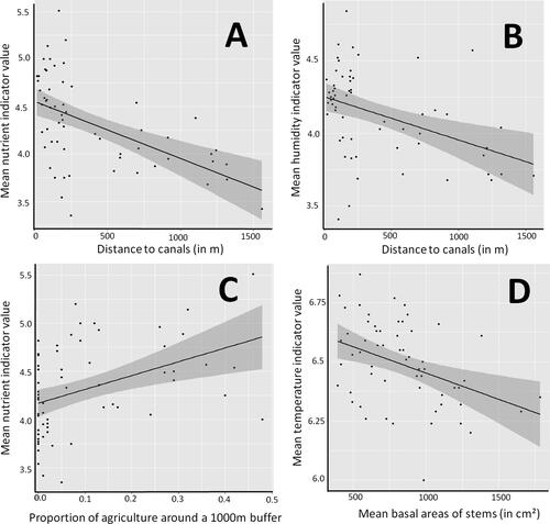
Table 4. Results of linear mixed effects models.

Response variable	Predictors (increasing values)	t Value	Standard error	p Value	Residual variation
Mean indicator value: humidity	Distance to canals	−3.21	0.07	.002	0.28
Mean indicator value: nutrients	Distance to canals	−5.19	0.1	<.001	0.39
Mean indicator value: nutrients	Proportion of agricultural areas	3.38	0.07	<.001	0.42
Mean indicator value: temperature	Mean basal area of trees	−3.23	<0.001	.002	0.16
Plant species richness	Wet, nutrient rich sites	−0.62	0.72	.54	5.51
	Cooler sites	0.88	0.75	.38	5.50
	High pH and soil salinity	−0.93	0.78	.36	5.50
	Old, open forest	0.80	0.73	.43	5.50
	Heterogeneous forest	0.86	0.72	.39	5.49
	Crown density	−0.24	0.72	.81	5.52
	Forest center sites	−0.76	0.72	.45	5.49
	Landscape heterogeneity	−0.20	0.76	.84	5.52
	Distance to canals	−3.60	0.69	<.001	5.16
Plant FDis	Wet, nutrient rich sites	−3.21	0.0008	.002	0.006
	Cooler sites	−0.92	0.0009	.36	0.007
	High pH and soil salinity	−1.87	0.0009	.07	0.007
	Old, open forest	−1.39	0.0009	.17	0.007
	Heterogeneous forest	3.65	0.0008	<.001	0.006
	Crown density	−1.53	0.0009	.13	0.007
	Forest center sites	−0.18	0.0009	.86	0.007
	Landscape heterogeneity	−0.08	0.0009	.94	0.007
	Distance to canals	−2.24	0.0008	.003	0.006
Widely distributed species	Landscape heterogeneity	2.3	0.04	.03	0.29
	Forest center sites	−0.73	0.04	.47	0.30
	Distance to canals	−0.45	0.04	.65	0.30
Mediterranean species	Landscape heterogeneity	−2.23	0.06	.03	0.40
	Forest center sites	1.34	0.05	.19	0.42
	Distance to canals	0.61	0.06	.54	0.42
Salt tolerant plants	Soil pH and salinity	−0.76	0.07	.45	0.50
	Distance to canals	−3.70	0.06	<.001	0.46

Random factor was always the reserve identity (PsV or PdC). Each row represents a separate statistical model. Plant species richness, plant FDdis, widely distributed species, Mediterranean species and salt tolerant species are only named once as response, but refer to all the predictors within the same box. Statistically significant relationships are printed in bold face.

The PCA of the six local factors resulted in three axes, which collectively captured 78% of total variance. The PCLoc1 axis can be interpreted as a gradient from dry and nutrient poor locations with open canopy to shady, humid and nutrient rich sites. The PCLoc2 axis mainly represents a gradient in temperature, while the PCLoc3 reflects the gradient in soil pH and salinity.

Among the six descriptors of forest stand structure, the three first PCs accounted for 79% of total variation. Here, PCFor1 depicts the gradient from dense forest stands with many small and young trees to more open and old grown forest locations with fewer, but taller stems. PCFor2 represents forest heterogeneity and PCFor3 represents tree crown density.

Finally, at the landscape level the first three PC axes summarized 89% of variation. PCLand1 mirrors the gradient from sites situated at the reserve edges (surrounded by high proportions of agricultural land and high landscape diversity) into the centers of the forest with high proportions of natural areas and lower habitat diversity around (because of the lack of modified landscape elements). PCLand2 represents landscape heterogeneity and diversity around the sites. PCLand3 can be interpreted as distance to canals. The main outcome of all three PCAs is summarized in Table 5.

Table 5. Factor loadings of the PC axes obtained from three separate PCAs for local, forest stand and landscape variables, respectively.

Local	PCLoc1 =Wet, nutrient rich sites	PCLoc2 =Cooler sites	PCLoc3 =High pH and soil salinity
pH	−0.06	−0.13	0.85
Salt	0.01	0.27	0.75
IV_Light	−0.89	0.13	0.00
IV_Temp	−0.09	−0.87	−0.09
IV_Humidity	0.71	0.59	0.06
IV_Nutrients	0.82	0.40	−0.11
Forest	PCFor1 =Old, open forest	PCFor2 =Heterogeneous forest	PCFor3 =High crown density
Tree height	0.85	−0.11	0.09
Standard deviation basal area	0.36	0.68	0.30
Crown density	−0.04	−0.02	0.94
Mean basal area	0.81	0.48	0.14
Forest density	−0.80	−0.13	0.34
Proportion of deciduous trees	0.08	−0.83	0.20
Landscape	PCLand1 =Site in center of forest	PCLand2 =Landscape heterogeneity	PCLand3 =Distance to canals
Distance to edges	0.89	−0.09	0.10
Distance to canals	0.12	−0.29	0.95
Edge density	0.04	0.90	−0.29
Landscape diversity	−0.65	0.65	−0.26
Natural areas	0.87	−0.39	0.12
Agricultural land	−0.81	−0.36	0.01

PC axes are named after the raw variables with the highest factor loadings and subsequent ecological interpretation. Factor loadings >0.6 are marked in bold. Ellenberg indicator values are abbreviated with IV.

GLMM results indicated that FDis decreased at more wet and nutrient rich sites and with lower forest heterogeneity (Table 4, Figure 3(A,B)). Furthermore, plant species richness and plant FDis per site were significantly related to the distance of sites to the nearest canal (Table 4, Figure 3(C)). All other tested site descriptors had no detectable influence on vascular plant richness or FDis.

Figure 2. Factors influencing mean Ellenberg indicator values for nutrient availability (A and C), humidity (B) and temperature (D) in 60 local species lists collated in the two reserves PsV and PdC. Dark grey shaded areas mark the 95% confidence bands of the linear regression (black line).

Figure 3. Factors influencing (A–C) plant functional dispersion (FDis), (D) proportion of salt tolerant species, (E) proportion of Mediterranean species, (F) proportion of widely distributed species in 60 local species lists collated in the two reserves PsV and PdC. Dark grey shaded areas mark the 95% confidence bands of the linear regression (black line).

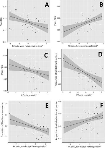
The proportion of salt tolerant species was not influenced by local salinity values taken from own soil measurements, but increased towards the canals (Figure 3(D), Table 4). The proportion of Mediterranean plant species declined with increasing landscape heterogeneity in the surroundings (Figure 3(E), Table 4), while widely distributed species increased (Figure 3(F), Table 4).

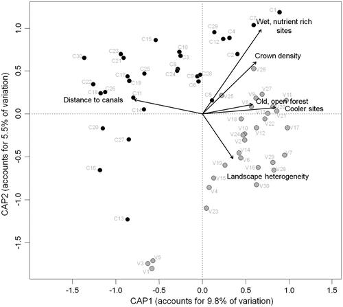
In contrast to the analyses of species richness or functional dispersion, all tested PC axes were significantly related to variation in local plant community composition. The position of sites along the humidity and nutrient gradient (p = .001) and its temperature conditions (p = .001) accounted for 8% of the observed variation. Forest age and density (p = .002) and crown density (p = .001) explained another 7.7%, while landscape heterogeneity (p = .001) and the distance to canals (p = .001) explained 7.8% of variation. Differences between the two reserves (p = .001) accounted for a further 4.6% of variation. So, altogether 28.2% of variation in local vascular plant species composition could be attributed to the seven factors chosen for matrix regression analysis, with local, forest stand and landscape factors all contributing in roughly equal manner (Figure 4). The CAP ordination further revealed two clusters clearly separating sites situated in PsV from those in PdC, what again underlines the difference in plant species composition between the two reserves. PdC sites were more scattered than PsV sites. Moreover, three PsV sites, viz. V1, V3 and V5, were clearly distinct from all other study sites in reduced ordination space. In PdC four locations, C13, C16, C20 and C27, clustered separately from the rest of all PdC sites (Figure 4). All these sites were characterized through very dry and nutrient poor conditions with low crown density.

Figure 4. Constrained ordination plot (canonical analysis of principal coordinates) of the plant community composition at 60 sites in the two pine forest reserves PsV and PdC. Included environmental variables are six (two each from local, forest stand and landscape aspects) of the nine PC axes representing the factors listed in Table 2. Locations in PsV colored in grey, locations in PdC in black.

Discussion

Even though our study sites were all located in stands of the same forest type on paleodunes, dominated by oak trees, our results showed substantial variation in the diversity and species composition of plant communities. We observed significant differences in mean plant species richness between PsV and PdC, with sites in PsV on average having more species. In contrast, estimated gamma diversity showed no such difference between the two reserves. Alien invasive species seem to date not problematic in the two reserves, as only seven alien species (e.g. Ailanthus altissima (Mill.) Swingle, Erigeron sumatrensis Retz., Robinia pseudoacacia L.) were found sporadically and never occurred in large numbers.

Species composition varied between PsV and PdC, although there was a large basic species pool which both reserves had in common. Overall, the species lists were dominated by plants widespread in Mediterranean ecosystems, but also a few internationally protected species (e.g. the orchids Anacamptis pyramidalis (L.) Rich., Anacamptis coriophora (L.) R.M.Bateman, Pridgeon & M.W.Chase, Anacamptis morio (L.) R.M.Bateman, Pridgeon & M.W.Chase, Neotinea tridentata (Scop.) R.M. Bateman, Pridgeon & M.W. Chase, Platanthera chlorantha (Custer) Rchb. and Serapias vomeracea Briq.) occurred in the reserves. Besides some xerophilous plant species like Hypochaeris radicata L., many of the PsV indicator species were hygrophilous like Populus alba L., Potentilla reptans L. and Prunella vulgaris L., while PdC indicator species often are bound to dry habitats like Phillyrea angustifolia L., Carex liparocarpos Gaudin and Quercus ilex L. So, local conditions in PsV may be characterized by higher humidity in comparison to PdC. However, there was no general difference in mean Ellenberg humidity values between PsV and PdC (Table 2).

Humidity and nutrient availability were significantly higher in proximity to the canals what indicates that they may contribute to eutrophication in these two Mediterranean coastal forests. Local nutrient availability inside the reserves increased with the proportion of agricultural areas around the study sites. Agricultural areas are known as major source of NOx pollution (Almaraz et al. 2018). The influence of fertilizers on plant communities has often been shown in agricultural environments (Van den Berge et al. 2019) and computer models (Kros et al. 2015). Moreover, atmospheric nitrogen deposition can influence biodiversity and change vegetation (Tilman and Isbell 2015; van Dobben and de Vries 2017). For our study region Lucialli et al. (2007) demonstrated the contribution of the industrial harbor and its traffic to air pollution, which might also influence the nearby forest reserve PsV. So, besides aquatic nutrient transport through the canals, airborne deposition of NOx from the harbor of Ravenna must be taken into account. The observed increase of nutrient indicating plants at sites with more agricultural areas in their vicinity indicate a strong influence of intensive land-use on protected areas, even with rather low proportions of agricultural areas (which never exceeded 48% of area in a 1000 m buffer).

Higher forest age (inferred from larger mean basal area of stems) was associated with lower temperature scores of the vegetation. This highlights the potential of old-growth forests to moderate microclimatic conditions and thereby even counteract adverse effects of climate change (Frey et al. 2016). Older forest stands also had higher structural heterogeneity. The biggest and probably oldest trees in the study area are stone pine trees (Pinus pinea L.), which build up an upper canopy layer above the tree crowns of oaks (Quercus sp. L.), ash trees (Fraxinus sp. L.) and poplars (mainly Populus alba L.). Ehbrecht et al. (2019) found that structural heterogeneity buffers the diurnal temperature variation in central European forests, and supposed that this effect might be even more pronounced in regions with low summer precipitation like the Mediterranean area. So, the observed lower temperature scores as inferred from plant indicator values might also be modulated by forest structural heterogeneity.

Plant species richness and FDis decreased with the distance of sites to canals. The canals as structural element break up the forest structure, enabling plant species dispersal and establishment of more light-demanding species. Furthermore, water is one of the limiting factors in dry Mediterranean ecosystems. Aridity is known to decrease plant richness and functional diversity at large scales and along with different management intensity (Rota et al. 2017; de la Riva et al. 2018). Close to the canals, constant water supply is ensured even in hot summer months like July and August. As a consequence, tree crown density increases as well as plant richness and functional diversity.

Otherwise, high humidity and especially nutrient availability can also decrease functional diversity and furthermore lead to functional homogenization (Helsen et al. 2014; Reinecke et al. 2014). Nitrogen deposition is a severe problem for terrestrial plant diversity, especially in the Mediterranean region (Bobbink et al. 2010). In line with this, also in our two forest reserves FDis decreased at humid and nutrient rich sites.

Another factor influencing plant FDis was forest heterogeneity. The more heterogeneous the forest stands around the location were, the more increased plant FDis. The “Forest heterogeneity” PC-axis mainly was determined by the standard deviation of stems and a decline in the proportion of deciduous trees. Some locations were characterized by very dense young tree stands with elms as dominating tree species. Here, forest stands often were very monotonous and showed low variety in available niches. In contrast, parts of the reserves where big and old pine trees could be found were often very heterogeneous in structure. Here, younger trees and bushes grow in between and also forest clearings exist on which sandy soils enable the establishment of diverse herbs. Therefore, structural heterogeneity seems to increase FDis, as with more structures more microhabitats are available.

Besides the positive aspects of water canals on plant richness and FDis, they also serve as source of soil salinity (Antonellini et al. 2008). Salt water intrusion and subsequent soil salinization is a severe environmental problem of the whole coastal region of the Emilia-Romagna, caused by land subsidence and ground water pumping which disturb the coastal hydraulic gradients and increase the influx of seawater (Mollema et al. 2013). In line with this, we detected a higher proportion of salt tolerant species near canals. In contrast, the PC-axis representing measured soil salinity did not correlate with the proportion of salt tolerant plants. Reasons for this might be the generally high soil salinity all over the reserves, with values between 1 and 25 g/l (Antonellini et al. 2008), leading to an all-over occurrence of salt tolerant plants inside the reserves. Indeed, we observed on average 9% salt tolerant species per location.

With regard to species distributional ranges, we found a significant decrease of Mediterranean species with higher landscape heterogeneity, whereas widely distributed species were concomitantly increasing. As landscape heterogeneity and diversity in our study were not only driven by the structure and number of natural habitats, but also strongly by the prevalence of modified landscape elements like buildings, gardens, agricultural areas, streets and hedges, we conclude that the disappearance of species with restricted distributional ranges is an effect of anthropogenic modification of the landscape. Land-use change is known as a severe constraint on Mediterranean coastal regions and its plant diversity and leads to the disappearance of coastal forests (Falcucci et al. 2007;; Hevia et al. 2016). Additionally, urban areas and other human modified landscapes are a source for alien and cosmopolitan plant species (Kühn et al. 2017). So, the landscape scale effect on the prevalence of plants with restricted Mediterranean ranges is in line with previous findings and expectations.

Canonical analysis of principal coordinates confirmed the differences in species composition between PsV and PdC. Old grown, rather open forest sites with lower temperature scores were more often found in PsV, while PdC locations were characterized by lower heterogeneity of the surrounding landscape and a larger distance to canals. So, water availability might be reduced in PdC, what might explain some difference in species composition, resulting in xerophilous plants contributing more to indicator species in PdC. Nevertheless, wet and nutrient rich sites, being similar in their species composition and indicating a basic common species pool, were found in both reserves. Species turnover was higher in PdC than in PsV resulting in a more scattered cluster of sites in the ordination plot compared to the more compact one of PsV. A slightly higher beta diversity might compensate the lower mean species richness per site in PdC, resulting in the equal total plant richness found in both reserves. Some locations of PsV and PdC were clearly distant to the main cluster. In PsV, especially sites V1, V3 and V5 formed a separate group. These locations were all situated in the north-west of PsV, where the forest is characterized by very dry conditions. These sites were chosen at small forest clearings due to limited accessibility, resulting in a relatively low crown density. There, sandy underground and grass vegetation could be found. However, these aspects are not exclusive for V1, V3 and V5, but also occurred at other study sites. Within PdC, sites C13, C16, C20 and C27 showed – analogous to the situation in PsV – some distance in plant species composition to the other PdC locations. Again, these sites were mainly situated on dry and sandy habitats with low crown density. But here the forest structure often was not as semi-natural as at the aforementioned PsV sites. Rather, sites C13, C16 and C20 were characterized by monotonous pine plantations (mainly Pinus sylvestris L., Pinus nigra J.F. Arnold and Pinus pinaster Ait., but not Pinus pinea L.) also resulting in another classification of their main habitat structure at official vegetation maps (Piccoli and Merloni 1999). This area has been planted only about 30 years ago, without taking into account conservation and biodiversity management practices (Enrica Burioli, pers. communication). These plantations, however, are today left unmanaged, resulting in a successive change in vegetation structure, with young oak trees now growing in between, such that forest structure approaches that of semi-natural mixed forest sites. There are also no clearings, but broad paths breaking up the monotonous plantation structure and enabling light-demanding herb and shrub layer species to grow. Another characteristic that all of these outlying sites (whether in PsV or PdC) had in common, is a relatively low nutrient availability, resulting in low mean nutrient-Ellenberg indicator values. Under a conservation perspective, these sites (V1, V3, V5, C13, C16, C20 and C27) are of high interest, because here species of dry and open, nutrient poor habitats (like Euphorbia cyparissias L., Helianthemum nummularium (L.) Mill., Sanguisorba minor Scop. and Teucrium chamaedrys L.) can be found. Furthermore, at all of these sites, protected orchid species can be found, underlining the importance of open forest structures.

Comparing the influence of local, forest stand and landscape scale attributes on plant community composition, each spatial aspect seemed to play an equally important role. In coastal dune habitats, Sperandii et al. (2019) detected local factors to be the most important drivers of species richness and focal species cover, while human mediated disturbance and landscape structure were less relevant. Here, the selective conditions of dune ecosystems as clear examples of habitat filtering favor the establishment of plant species especially adapted to this environment. For coastal forest habitats, where local conditions are not this extreme, there appears to be no such weighting on one of the observed spatial aspects. Rather, all spatial scales are important for determining local community assembly. So, forest management and conservation practices alone cannot preserve plant communities without taking landscape structure into account (Vellend et al. 2017). In return, landscape structure is also not the dominant source of plant community variation inside these two forest reserves.

Conclusion

Local, land-use history driven and landscape-scale effects equally shape local plant composition in the two forest reserves under study. Therefore, all spatial scales, as well as land-use history should be taken into account for effective conservation practices. Forest clearings and other open forest structures were important habitats inside the coastal forest reserves, which most likely comprised fractions of the ancient plant communities. Such dry and open, sandy, nutrient poor habitats might once have been found throughout the paleodune habitats, but nowadays are endangered through nutrient spill-over and natural succession. Nutrient import seems to mainly occur through water canals and from the agricultural landscape around the reserves. So, the landscape scale here plays an important role in driving eutrophication of terrestrial habitats, what finally leads to lower plant functional dispersion. The proportion of modified areas also leads to the replacement of genuinely Mediterranean species through more widely distributed ones. Here, land-use and landscape scale characteristics clearly seem to drive biotic homogenization also inside protected, but isolated coastal forest reserves.

Acknowledgements

We are grateful to Angela Vistoli and Corbaro Lamberto (Comune di Ravenna) for providing permits and to Enrica Burioli for valuable information on the land-use history of the study area. We thank Giorgio Lazzari for his help with identifying some difficult plant specimens. We are also thankful to Carina Betz, Annika Goßmann, Hannah Reith and Constanze Fett for assistance with sampling field data. We also like to thank the anonymous reviewers which helped improving our manuscript through their constructive comments.

Disclosure statement

No potential conflict of interest was reported by the authors.

Additional information

Funding

Financial support was kindly provided to Britta Uhl by the Heinrich Böll Stiftung and through funds of the Faculty of Life Sciences, University of Vienna.

References

- Acta Plantarum. 2007. [accessed 2019 April]. http://www.actaplantarum.org/home/utilities.php.
- Aichele D, Schwegler HW, Bachofer M. 1998. Unsere Gräser [Our grasses]. Stuttgart: Franckh-Kosmos Verlags-GmbH & Co.
- Almaraz M, Bai E, Wang C, Trousdell J, Conley S, Faloona I, Houlton BZ. 2018. Agriculture is a major source of NOx pollution in California. Sci Adv. 4(1):eaao3477.
- Amici V, Rocchini D, Filibeck G, Bacaro G, Santi E, Geri F, Landi S, Scoppola A, Chiarucci A. 2015. Landscape structure effects on forest plant diversity at local scale: exploring the role of spatial extent. Ecol Complex. 21:44–52.
- Andreatta G. 2010. Proposta Di Un ‘silvomuseo’ Nelle Pinete Storiche Di Ravenna [Proposal for a ‘sylvomuseum’ in the historic pine forests of Ravenna]. Forest@ – J Silviculture Forest Ecol. 7(6):237–246.
- Antonellini M, Mollema P, Giambastiani B, Bishop K, Caruso L, Minchio A, Pellegrini L, Sabia M, Ulazzi E, Gabbianelli G. 2008. Salt water intrusion in the coastal aquifer of the southern Po plain. Hydrogeol J. 16(8):1541–1556.
- Araújo MB, Lobo JM, Moreno JC. 2007. The effectiveness of Iberian protected areas in conserving terrestrial biodiversity. Conserv Biol. 21(6):1423–1432.
- Assemblea legislativa della Regione Emilia-Romagna. 1988. Legge regionale 2 juglio 1988, n. 27, Istituzione del parco regionale del delta del po [regional law from 2 june 1988, n.27, Institution of the regional park “Po delta”]; [accessed 2019 September]. http://demetra.regione.emilia-romagna.it/al/articolo?urn=er:assemblealegislativa:legge:1988;27.
- Bassi A. 2004. Guida alle flora della Pineta San Vitale [Guide to the flora of Pineta san Vitale]. Ravenna (IT): A. Longo Editore snc.
- Bazzichetto M, Malavasi M, Barták V, Acosta ATR, Moudrý V, Carranza ML. 2018. Modeling plant invasion on Mediterranean coastal landscapes: an integrative approach using remotely sensed data. Landscape Urban Plann. 171:98–106.
- Bird Life International. 2019. Important bird areas factsheet: Punte Alberete and Valle della Canna, Pineta san Vitale and Pialassa della Baiona; [accessed 2019 January]. http://www.birdlife.org.
- Blondel J. 2006. The ‘Design’ of Mediterranean landscapes: a millennial story of humans and ecological systems during the historic period. Hum Ecol. 34(5):713–729.
- Bobbink R, Hicks K, Galloway J, Spranger T, Alkemade R, Ashmore M, Bustamante M, Cinderby S, Davidson E, Dentener F, et al. 2010. Global assessment of nitrogen deposition effects on terrestrial plant diversity: a synthesis. Ecol Appl. 20(1):30–59.
- Böhling N. 1995. Zeigerwerte der Phanerogamen-Flora von Naxos (Griechenland). Ein Beitrag zur ökologischen Kennzeichnung der mediterranen Pflanzenwelt [Indicator values of phanerogame flora of Naxos (Greece). A contribution to the ecological characteristics of the Mediterranean flora]. Stuttgarter Beiträge Zur Naturkunde Serie A. 533:1–27.
- Bryant DM, Ducey MJ, Innes JC, Lee TD, Eckert RT, Zarin DJ. 2005. Forest community analysis and the point-centered quarter method. Plant Ecol. 175(2):193–203.
- Burnie D. 2007. Mediterrane Wildpflanzen [Mediterranean plants]. München: Dorling Kindersley Verlag GmbH.
- Burrascano S, Ripullone F, Bernardo L, Borghetti M, Carli E, Colangelo M, Gangale C, Gargano D, Gentilesca T, Luzzi G, et al. 2018. It’s a long way to the top: plant species diversity in the transition from managed to old-growth forests. J Veg Sci. 29(1):98–109.
- Buscaroli A, Dinelli E, Zannoni D. 2011. Geohydrological and environmental evolution of the area included among the lower course of the Lamone River and the Adriatic Coast. Environ Qual. 5:11–22.
- Bussotti F, Gerosa G. 2002. Are the Mediterranean forests in southern Europe threatened from ozone? J Mediterr Ecol. 3(2–3):23–34.
- Chao A, Ma KH, Hsieh TC. 2016. iNEXT (iNterpolation and EXTrapolation) Online: Software for interpolation and extrapolation of species diversity; [accessed 2019 January]. http://chao.stat.nthu.edu.tw/wordpress/software_download/.
- Clavel J, Julliard R, Devictor V. 2011. Worldwide decline of specialist species: toward a global functional homogenization? Front Ecol Environ. 9(4):222–228.
- Clément F, Ruiz J, Rodríguez MA, Blais D, Campeau S. 2017. Landscape diversity and forest edge density regulate stream water quality in agricultural catchments. Ecol Indic. 72:627–639.
- Cowling RM, Rundel PW, Lamont BB, Arroyo MK, Arianoutsou M. 1996. Plant diversity in Mediterranean-climate regions. Trends Ecol Evol. 11(9):362–366.
- Cuttelod A, García N, Malak DA, Temple HJ, Katariya V. 2009. The Mediterranean: a biodiversity hotspot under threat. In: Vié J-C, Hilton-Taylor C, Stuart SN, editors. Wildlife in a changing world – an analysis of the 2008 IUCN Red List of threatened species. Gland: IUCN; p. 89–101.
- de la Riva EG, Violle C, Pérez-Ramos IM, Marañón T, Navarro-Fernández CM, Olmo M, Villar R. 2018. A multidimensional functional trait approach reveals the imprint of environmental stress in Mediterranean woody communities. Ecosystems. 21(2):248–262.
- Doxa A, Albert CH, Leriche A, Saatkamp A. 2017. Prioritizing conservation areas for coastal plant diversity under increasing urbanization. J Environ Manage. 201:425–434.
- Ehbrecht M, Schall P, Ammer C, Fischer M, Seidel D. 2019. Effects of structural heterogeneity on the diurnal temperature range in temperate forest ecosystems. For Ecol Manage. 432:860–867.
- Ellenberg H, Leuschner C. 2010. Vegetation Mitteleuropas mit den Alpen [Vegetation of central Europe including the Alps]. Stuttgart: Ulmer.
- Falcucci A, Maiorano L, Boitani L. 2007. Changes in land-use/land-cover patterns in Italy and their implications for biodiversity conservation. Landscape Ecol. 22(4):617–631.
- Flückiger W. 2007. Wirkung von Streusalz auf Forstgehölze [Effect of salt on forest trees]. [accessed 2019 April]:[10 p.]. www.iap.ch/publikationen/zusammenfassung_salzversuche.pdf.
- Frey SJK, Hadley AS, Johnson SL, Schulze M, Jones JA, Betts MG. 2016. Spatial models reveal the microclimatic buffering capacity of old-growth forests. Sci Adv. 2(4):e1501392.
- Geri F, Amici V, Rocchini D. 2010. Human activity impact on the heterogeneity of a Mediterranean landscape. Appl Geogr. 30(3):370–379.
- Helsen K, Ceulemans T, Stevens CJ, Honnay O. 2014. Increasing soil nutrient loads of European semi-natural grasslands strongly alter plant functional diversity independently of species loss. Ecosystems. 17(1):169–181.
- Hevia V, Carmona CP, Azcárate FM, Torralba M, Alcorlo P, Ariño R, Lozano J, Castro-Cobo S, González JA. 2016. Effects of land use on taxonomic and functional diversity: a cross-taxon analysis in a Mediterranean landscape. Oecologia. 181(4):959–970.
- Infoflora. 2004. Genf: Stefan Eggenberg; [accessed 2019 April]. https://www.infoflora.ch/de/.
- Kros J, Bakker MM, Reidsma P, Kanellopoulos A, Alam SJ, de Vries W. 2015. Impacts of agricultural changes in response to climate and socioeconomic change on nitrogen deposition in nature reserves. Landscape Ecol. 30(5):871–885.
- Kühn I, Wolf J, Schneider A. 2017. Is there an urban effect in alien plant invasions? Biol Invasions. 19(12):3505–3513.
- Laliberté E, Legendre P. 2010. A distance-based framework for measuring functional diversity from multiple traits. Ecology. 91(1):299–305.
- Laliberté E, Legendre P, Shipley B. 2014. Package ‘FD’: Measuring functional diversity from multiple traits, and other tools for functional ecology. R package version 1.0-12; [accessed 2019 April]. https://cran.r-project.org/web/packages/FD/FD.pdf.
- Lavergne S, Thuiller W, Molina J, Debussche M. 2005. Environmental and human factors influencing rare plant local occurrence, extinction and persistence: a 115-year study in the Mediterranean region. J Biogeogr. 32(5):799–811.
- Liu D, Ogaya R, Barbeta A, Yang X, Peñuelas J. 2018. Long-term experimental drought combined with natural extremes accelerate vegetation shift in a Mediterranean holm oak forest. Environ Exp Bot. 151:1–11.
- Lucialli P, Ugolini P, Pollini E. 2007. Harbour of Ravenna: the contribution of harbour traffic to air quality. Atmos Environ. 41(30):6421–6431.
- Luzuriaga AL, Sánchez AM, López-Angulo J, Escudero A. 2018. Habitat fragmentation determines diversity of annual plant communities at landscape and fine spatial scales. Basic Appl Ecol. 29:12–19.
- Malavasi M, Santoro R, Cutini M, Acosta ATR, Laura Carranza M. 2016. The impact of human pressure on landscape patterns and plant species richness in Mediterranean coastal dunes. Plant Biosystems. 150(1):73–82.
- Malfitano A. 2002. Alle origini della politica di tutela ambientale in Italia. Luigi Rava e la nuova Pineta ‘Storica’ di Ravenna [At the origins of environmental protection policy in Italy. Luigi Rava and the new “Historical” Pinewood of Ravenna]. Storia e Futuro. 1:1–18.
- Malicki MA, Walczak RT. 1999. Evaluating soil salinity status from bulk electrical conductivity and permittivity. Eur J Soil Sci. 50(3):505–514.
- Merloni N, Piccoli F, cartographers. 1999. Carta della vegetazione - Parco Regionale del Delta del Po – Stazione Pineta di san Vitale e Piallasse di Ravenna (Digitale) [Vegetation map – Regional park Po Delta – Pineta di san Vitale and Piallasse of Ravenna] [vegetation map]; [accessed 2019 April]. https://geoportale.regione.emilia-romagna.it.
- Mitchell K. 2010. Quantitative analysis by the Point-Centered Quarter method. [accessed 2019 April]:[56 p.]. arXiv preprint arXiv:1010.3303.
- Molina-Venegas R, Aparicio A, Lavergne S, Arroyo J. 2016. How soil and elevation shape local plant biodiversity in a Mediterranean hotspot. Biodivers Conserv. 25(6):1133–1149.
- Mollema PN, Antonellini M, Dinelli E, Gabbianelli G, Greggio N, Stuyfzand PJ. 2013. Hydrochemical and physical processes influencing salinization and freshening in Mediterranean low-lying coastal environments. Appl Geochem. 34:207–221.
- Musolino D, Vezzani C, Massarutto A. 2019. Drought management in the Po river basin, Italy. In: Iglesias A, Assimacopoulos D, Van Lanen HAJ, editors. Drought: science and policy. Chichester (UK): John Wiley & Sons, Ltd.; p. 201–215.
- Myers N, Mittermeier RA, Mittermeier CG, da Fonseca GAB, Kent J. 2000. Biodiversity hotspots for conservation priorities. Nature. 403(6772):853–858.
- Oksanen J, Guillaume Blanchet F, Friendly M, Kindt R, Legendre P, McGlinn D, Minchin PR, O’Hara RB, Simpson GL, Solymos P. 2018. Vegan: community ecology package. R package version 2.5 – 2; [accessed 2019 April]. https://cran.r-project.org/package=vegan.
- Peñuelas J, Sardans J, Filella I, Estiarte M, Llusià J, Ogaya R, Carnicer J, Bartrons M, Rivas-Ubach A, Grau O, et al. 2018. Assessment of the impacts of climate change on Mediterranean terrestrial ecosystems based on data from field experiments and long-term monitored field gradients in Catalonia. Environ Exp Bot. 152:49–59.
- Piccoli F, Merloni N, cartographers. 1999. Carta della vegetazione – Parco Regionale del Delta del Po – Stazione Pineta di Classe e Saline di Cervia (Digitale) [Vegetation map – Regional park Po Delta – Pineta di Classe and Saline of Cervia] [vegetation map]; [accessed 2019 April]. https://geoportale.regione.emilia-romagna.it.
- Pignatti S, Menegoni P, Pietrosanti S. 2005. Valori di bioindicazione delle piante vascolari della flora d’Italia [Bioindicator values of vascular plants of the Flora of Italy]. Braun-Blanquetia. 39:3–95.
- Pinheiro J, Bates D, Debroy S, Sarkar D, R Core Team. 2018. _nlme: Linear and Nonlinear Mixed Effects Models_. R Package Version 3.1-137; [accessed 2019 April]. https://cran.r-project.org/package=nlme.
- QGIS Development Team. 2018. QGIS Geographic Information System. Open Source Geospatial Foundation Project; [accessed 2018 January]. http://qgis.osgeo.org.
- Reinecke J, Klemm G, Heinken T. 2014. Vegetation change and homogenization of species composition in temperate nutrient deficient Scots pine forests after 45 yr. J Veg Sci. 25(1):113–121.
- Revelle W. 2017. psych: procedures for personality and psychological research; [accessed 2019 April]. https://CRAN.R-project.org/package=psychVersion=1.8.4.
- Roberts DW. 2016. Labdsv.: Ordination and multivariate analysis for ecology. R package version 1.8-0; [accessed 2019 April]. https://cran.r-project.org/package=labdsv.
- Rosati L, Fipaldini M, Marignani M, Blasi C. 2010. Effects of fragmentation on vascular plant diversity in a Mediterranean forest archipelago. Plant Biosyst. 144(1):38–46.
- Rota C, Manzano P, Carmona CP, Malo JE, Peco B. 2017. Plant community assembly in Mediterranean grasslands: understanding the interplay between grazing and spatio-temporal water availability. J Veg Sci. 28(1):149–159.
- Sabatini FM, Burton JI, Scheller RM, Amatangelo KL, Mladenoff DJ. 2014. Functional diversity of ground-layer plant communities in old-growth and managed northern hardwood forests. Appl Veg Sci. 17(3):398–407.
- Schaffers AP, Sýkora KV. 2000. Reliability of Ellenberg indicator values for moisture, nitrogen and soil reaction: a comparison with field measurements. J Veg Sci. 11(2):225–244.
- Schindler S, von Wehrden H, Poirazidis K, Hochachka WM, Wrbka T, Kati V. 2015. Performance of methods to select landscape metrics for modelling species richness. Ecol Modell. 295:107–112.
- Schneider CA, Rasband W, Eliceiri K. 2012. NIH Image to ImageJ: 25 years of image analysis. Nat Methods. 9(7):671–675.
- Schönfelder I, Schönfelder P. 2011. Kosmos Atlas Mittelmeer- und Kanarenflora [Mediterranean and canary island flora]. Stuttgart: Franckh-Kosmos Verlags-GmbH & Co.KG.
- Senghas K, Seybold S. 2003. Schmeil-Fitschen Flora von Deutschland [Flora of Germany]. Wiebelsheim: Quelle & Meyer Verlag GmbH & Co.
- Sperandii MG, Bazzichetto M, Acosta ATR, Barták V, Malavasi M. 2019. Multiple drivers of plant diversity in coastal dunes: a Mediterranean experience. Sci Total Environ. 652:1435–1444.
- Teixido AL, Quintanilla LG, Carren F, Gutiérrez D. 2010. Impacts of changes in land use and fragmentation patterns on Atlantic coastal forests in northern Spain. J Environ Manage. 91(4):879–986.
- Tilman D, Isbell F. 2015. Biodiversity: recovery as nitrogen declines. Nature. 528(7582):336–337.
- Tsiafouli MA, Monokrousos N, Sgardelis SP. 2018. Drought in spring increases microbial carbon loss through respiration in a Mediterranean pine forest. Soil Biol Biochem. 119:59–62.
- UNESCO. 2015. Bonn: Po Delta, United Nations Educational Scientic and Cultural Organisation; [accessed 2019 April]. https://www.unesco.org/new/en/natural-sciences/environment/ecological-sciences/biospherereserves/europe-north-america/italy/po-delta/.
- Van den Berge S, Tessens S, Baeten L, Vanderschaeve C, Verheyen K. 2019. Contrasting vegetation change (1974–2015) in hedgerows and forests in an intensively used agricultural landscape. Appl Veg Sci. 22(2):269–281.
- van Dobben HF, de Vries W. 2017. The contribution of nitrogen deposition to the eutrophication signal in understorey plant communities of European forests. Ecol Evol. 7(1):214–227.
- Vellend M, Baeten L, Becker-Scarpitta A, Boucher-Lalonde V, McCune JL, Messier J, Myers-Smith IH, Sax DF. 2017. Plant biodiverity change across scales during the Anthropocene. Annu Rev Plant Biol. 68(1):563–586.
- Warton DI, Hui F. 2011. The Arcsine is asinine: the analysis of proportions in ecology. Ecology. 92(1):3–10.
- Wickham H. 2016. ggplot2: elegant graphics for data analysis. New York (NY): Springer-Verlag.
- Wölfling M, Uhl B, Fiedler K. 2019. Multi-decadal surveys in a Mediterranean forest reserve – do succession and isolation drive moth species richness? Nat Conserv. 35:25–40.
- Wuyts K, de Schrijver A, Staelens J, Verheyen K. 2013. Edge effects on soil acidification in forests on sandy soils under high deposition load. Water Air Soil Pollut. 224(6):1–14.