Environmental factors influencing the distribution of habitat types in the highlands of the Kamnik − Savinja Alps

Abstract

In this work, we investigated the relationship between habitat types (HTs) and selected environmental factors in the highlands at altitudes of 1800–2558 m in the Kamnik-Savinja (KS) Alps in Slovenia. For 275 sampling sites, we identified seven HTs in their typical form and 11 ecotones, and provided field and modelled data for 14 environmental factors. HTs-environment relationships were analysed using multivariate ordination methods. In addition, binomial generalised linear mixed models were applied to reveal the influence of environmental factors on the occurrence of most frequent HTs in the study area [Outer Alpine Pinus mugo scrub (EUNIS code F2.4/Natura 2000 code 4070*), Southern rusty sedge grasslands (E4.413/6170), Cushion sedge carpets (E4.433/6170) and Fine calcareous screes (H2.43/8120)]. Results showed that certain modelled data (e.g. average annual air temperature) combined with field measurements (e.g. inclination, soil surface and soil moisture) can be effective predictors of most representative HTs in the study area, and thus useful for further refining of monitoring. Our study contributes to the knowledge and understanding of the relationships between environmental conditions and the occurrence of highland HTs in KS Alps, which probably concerns a great part of the Alpine highlands. Such knowledge is essential for assessing credible long-term conservation planning.

Keywords:

• Alpine habitat types
• multivariate analysis
• Pinus mugo
• alpine and subalpine calcareous grasslands
• Natura 2000
• Slovenia

Introduction

The Alps are the most prominent mountain range system in Europe and are of great concern in nature conservation issues because of their high proportion of endemic species (Aeschimann et al. 2004). The alpine landscape is characterised by topographically induced mosaics of microclimatic conditions, which are associated with local distribution of plant species (Scherrer and Körner 2011). In general, the Alpine biota is relatively wellstudied (e.g. Väre et al. 2003; Casazza et al. 2008; Dirnböck et al. 2011) and several studies have addressed the relationships between biota and environmental conditions (e.g. Reutter et al. 2003; Kryštufek et al. 2015; Rosbakh et al. 2015; Mathar et al. 2016; Novak et al. 2017). In nature conservation areas, such knowledge is particularly valued as this is the basic information needed to understand community distribution patterns.

In the Habitats Directive (Directive 1992/43/EEC), standardised ‘habitat types’ (hereafter HTs) are defined by characteristic species assemblages and abiotic conditions. Because plant communities are much more thoroughly studied than other biota, terrestrial HTs used in various classification schemes, are often based on phytosociological vegetation types, e.g. in the European Habitats Directive (Directive 1992/43/EEC) Annex I habitat types and the EUNIS (European Nature Information System) habitat classification (Devilliers and Devilliers-Terschuren 1996; EUR27 2007; Moss 2008; Tomaselli et al. 2013; Chytrý et al. 2020). Plant associations also relate to many other species, e.g. butterflies (Pellissier et al. 2013; Leingärtner et al. 2014; Čelik et al. 2015), but not to some others, e.g. harvestmen (Novak et al. 2017). However, studies on congruent variation in species richness patterns in alpine habitats are scarce (Finch and Löffler 2010). Consequently, the influence of invertebrates, associated with specific HTs, on the assemblage structure is poorly understood (Holmquist et al. 2011).

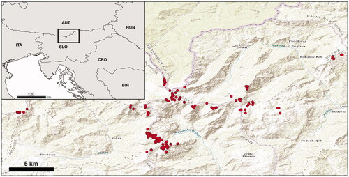
Since 2004, the Kamnik-Savinja (KS) Alps (Figure 1) in northern-central Slovenia have been a constituent part of the Natura 2000 Network (Official Gazette 45/2004), and thus of special interest for nature conservation concerns. This mountain group provides a range of alpine calcareous habitats, with species and HTs listed in Annexes I and II of the Habitats Directive (Directive 1992/43/EEC). There, abiotic conditions are similar to those in other calcareous Alps, especially the Julian Alps, but differ from them by significantly lower precipitation, and partly different plant communities (Seliškar 1998), which include some endemic species (Hegi et al. 1980; Martinčič et al. 1999; Wraber 2006). The upper limit of the montane zone is defined by the timberline, where altitudes range from 1700 to 1900 m. The timberline vegetation consists of Alpine and Carpathian subalpine Picea forests (EUNIS habitat code G3.1B, Natura 2000 habitat code 9410) dominated by Picea abies (L.) H. Karst. (Juvan et al. 2013). The second most important tree species is Larix decidua Mill., which occurs at elevations up to 2000 m a.s.l. Above the timberline, there is the subalpine zone. It refers to an intermediate belt between the montane and alpine vegetation zones and is characterised by Outer Alpine Pinus mugo Turra scrub (EUNIS habitat code F2.42, Natura 2000 code 4070*) (Šibík et al. 2010). The alpine zone is on average above 2000 m (Martinčič et al. 1999; Wraber 2006). Various calcareous alpine and subalpine grassland types occur on base-rich soils (EUNIS habitat code E4.4, Natura 2000 habitat code 6170), mainly from the Elyno-Seslerietea Br.-Bl. 1948 phytosociological class (Šilc and Čarni 2012). In the lower alpine zone, continuous Southern rusty sedge grasslands occur, with Carex sempervirens Vill., C. ferruginea Scop., and Festuca laxa Host on screes. With increasing altitude, the proportion of bare rocky surface, taluses, alpine grasslands, and snow habitats increases. Basic and ultra-basic inland cliffs (EUNIS habitat code H3.2, Natura 2000 habitat code 8210) host fragments of specific plant associations, such as Potentillo clusianae-Campanuletum zoysii Aichinger 1933 and Potentilletum nitidae Wikus 1959 (order Potentilletalia caulescentis Br.-Bl. in Br.-Bl. et Jenny 1926, class Asplenietea trichomanis (Br.-Bl. in Meier & Br.-Bl. 1934) Oberd. 1977). Calcareous and calcshist screes of the montane to alpine levels (EUNIS habitat code H2.43, Natura 2000 habitat code 8120) provide a habitat for various plant communities from the order Thlaspietalia rotundifolii Br.-Bl. in Br.-Bl. & Jenny 1926. Alpine grasslands in the KS Alps, such as the associations Ranunculo hybridi-Caricetum sempervirentis Poldini & Feoli Chiapella in Feoli Chiapella & Poldini 1993 (alliance Caricion austroalpinae Sutter 1962), Caricetum ferrugineae Lüdi 1921 (alliance Caricion ferrugineae Br.-Bl. 1931), Primulo carniolicae-Caricetum firmae Dakskobler 2006 and Gentiano terglouensis–Caricetum firmae T. Wraber 1970 (alliance Caricion firmae Gams 1936), are covered with snow for only a short period and are well adapted to gales and low temperatures (Lippert 1987). On snow-covered grasslands, taluses and stony habitats saturated with snow-water, only snow-patch plant communities (EUNIS habitat code E4.12) that persist for one to two months develop. Such are the associations Saxifrago sedoidis-Arabidetum caeruleae T. Wraber 1972 nom. ined. and Potentillo dubiae-Homogynetum discoloris Aichinger 1933 (order Arabidetalia caeruleae Rübel ex Br.-Bl. 1948) (Wraber 2006; Šilc and Čarni 2012).

Figure 1. Sampling map of habitat types in the alpine belt (spots) of the Kamnik–Savinja Alps.

Research and monitoring are two of the most important initiatives that should be implemented in alpine and subalpine vegetation communities, which are among the conservation priorities (García-González 2008). While the flora and distribution of plant communities in the KS Alps are well-researched (e.g. Seliškar 1998; Martinčič et al. 1999; Jogan et al. 2004; Wraber 2006; Martinčič 2008), the main environmental factors affecting their distribution have not been studied. In this respect, the main objective of our study was to investigate the relationship between HTs and selected abiotic factors in the highlands of the KS Alps at altitudes of 1800–2558 m. For this purpose, we focussed on the following question: which environmental factors influence the variability of habitat types in the target area?

Materials and methods

Study site

The KS Alps (Figure 1) are the southeasternmost part of the Alps (Gams and Vrišer 1998; Ogrin and Plut 2009) measuring ca. 900 km², of which modestly inclined southern slopes constitute the largest part, the highest peak being Mt. Grintovec, 2558 m (PZS 1998). The KS Alps are divided into the western group, i.e. the Mt. Storžič group; the central group, i.e. the Grintovci Mts. Group; and the eastern group, i.e. the Mt. Mrzla gora − Mt. Raduha group protruding to the east in the highland plateaus of Dleskovška planota and Mt. Velika planina (Marušič et al. 1998). Geologically, the KS Alps are a constituent part of the Adriatic microplate, which is a part of the African tectonic plate, and are composed mostly of Devonian and Triassic limestones (Celarc 2004; Ogrin and Plut 2009). High rock walls, taluses sloping by 20–37° (Kladnik 1981) and highland grasslands are the most characteristic habitats, with lithosols and rendzinas as the most frequent soils (GERK 2010). The climate is moderately alpine, with average annual temperatures decreasing from 6 °C to 0 °C, and average precipitation increasing from 1800 to 2600 mm at altitudes of 1800–2558 m. The snow cover persists for up to 200 days, and the average wind velocity exceeds 5 m s⁻¹ on the most exposed peaks (ARSO 2010). There is a range of characteristic subalpine (at altitudes of 1700–2000 m) and alpine (above 2000 m) HTs (Jogan et al. 2004) on lithosols and rendzinas (GERK 2010).

Field-based sampling

In the summer and early autumn of 2009 and 2013, after at least two days without rain and/or strong wind, we investigated a total of 275 sampling sites in a relatively narrow highland belt at altitudes of 1800–2558 m on the following 24 mountains (Figure 1): Brana, Grintovec, Kalški greben, Kočna, Kompotela, Koren, Koroška Rinka, Košutna, Kranjska Rinka, Krofička, Lučki Dedec, Mala Koroška Baba, Mala Ojstrica, Mokrica, Mrzla gora, Ojstrica, Planjava, Raduha, Skuta, Storžič, Štajerska Rinka, Turska gora, Velika Koroška Baba, Veliki Zvoh and on the Leskovška planota subalpine plateau. Sampling sites were selected according to the following scheme: we started sampling at 1800 m, continued at intervals of 100 m or less on the mountain top in all main directions (N, E, S and W) where conditions permitted, and ended at the summit. At each site, an area of 100 m² was surveyed as a 10 m × 10 m sampling plot. In each plot, the HT was identified using expert knowledge. For the identification of HTs, the Palaearctic habitat classification scheme (Devilliers and Devilliers-Terschuren 1996; EUR27 2007) was used, adapted for use in Slovenia (Jogan et al. 2004). This classification scheme is based on the phytosociological approach and is linked to the Natura 2000 Annex I of the 92/43/EEC Directive and to the European Nature Information System (EUNIS) habitat classification schemes (Tomaselli et al. 2013). For the purposes of this work, Palaearctic habitat classification codes were translated to both Annex I of Habitats Directive and Eunis Code. Where different HTs were present at the same altitude, we sampled all of them, with the exception of precipitous walls. Ecotones, considered here as interfacing HTs between typical HTs, were treated separately during field mapping as plots sharing more than a third of another HT. All HTs and ecotones recorded are listed in Table 1. Plants were identified using the keys and descriptions in Hegi et al. (1980), Lippert (1987), Martinčič et al. (1999), Lauber and Wagner (2001) and Wraber (2006). Taxonomic nomenclature for plant species followed Martinčič et al. (2007) and syntaxonomic nomenclature followed Šilc and Čarni (2012).

Table 1. Habitat types (HTs) and their ecotones (18 units) according to the EUNIS/Natura 2000 classification schemes and Palaearctic code from 275 sampled sites in the KS Alps.

EUNIS/Natura 2000 code; * a priority habitat	Palaearctic habitat code	Number of sampled plots	EUNIS habitat name
F2.42/4070*	31.52	28	Outer Alpine Pinus mugo scrub
F2.42 × E4.413/4070* × 6170	31.52 × 36.413	60	Outer Alpine Pinus mugo scrub × Southern rusty sedge grasslands
F2.42 × H2.43/4070* × 8120	31.52 × 61.23	1	Outer Alpine Pinus mugo scrub × Fine calcareous screes
F2.42 × H3.2/4070* × 8210	31.52 × 62.1	2	Outer Alpine Pinus mugo scrub × Basic and ultra-basic inland cliffs
E4.12	36.12	16	Boreo-alpine calcicline snow-patch grassland and herb habitats
E4.12 × E4.413/6170	36.12 × 36.413	4	Boreo-alpine calcicline snow-patch grassland and herb habitats × Southern rusty sedge grasslands
E4.12 × E4.433/6170	36.12 × 36.433	1	Boreo-alpine calcicline snow-patch grassland and herb habitats × Cushion sedge carpets
E4.12 × H2.43/8120	36.12 × 61.23	1	Boreo-alpine calcicline snow-patch grassland and herb habitats × Fine calcareous screes
E4.413/6170	36.413	30	Southern rusty sedge grasslands
E4.413 × H2.43/6170 × 8120	36.413 × 61.23	6	Southern rusty sedge grasslands × Fine calcareous screes
E4.413 × H3.2/6170 × 8210	36.413 × 62.1	2	Southern rusty sedge grasslands × Basic and ultra-basic inland cliffs
E4.433/6170	36.433	44	Cushion sedge carpets
E4.433 × H2.43/6170 × 8120	36.433 × 61.23	47	Cushion sedge carpets × Fine calcareous screes
E4.433 × H3.2/6170 × 8210	36.433 × 62.1	2	Cushion sedge carpets × Basic and ultra-basic inland cliffs
E4.52	36.52	4	Rough hawkbit (Leontodon hispidus) pastures
H2.43/8120	61.23	24	Fine calcareous screes
H2.43 × H3.2/8120 × 8210	61.23 × 62.1	1	Fine calcareous screes × Basic and ultra-basic inland cliffs
H3.2/8210	62.1	1	Basic and ultra-basic inland cliffs

For each sampling site, we provided field and modelled data for 14 environmental factors (Table 2). The altitude was determined using a Garmin GPSMAP 60CS navigation device (horizontal and vertical accuracies ± 3 m each), and azimuth and the average inclination were determined using a geological compass. Vegetation cover was estimated using a seven-point cover-abundance scale according to Braun-Blanquet (1964). Soil properties were determined using selected and partly simplified descriptors (FAO 2006; FAO et al. 2012). When squeezed between fingers, wet soils squeezed out the water, moist ones retained their shape without releasing any water and the dry ones were dusty. In substrate consistency, compact substrates were considered those with crustaceous soils or tightly embedded stones. Soil surface structure was considered heterogeneous if it consisted of two or three of the following components, each comprising at least one-third of the habitat: soil, stones greater than 5 cm in diameter, and monoliths, marl, rock walls, fissures, detritus and plant patches. Rockiness referred to at least 1 m high walls in the habitat.

Table 2. Environmental factors, their abbreviations as used in the figures, and classes considered in the investigation.

Environmental factor	Abbreviation (factor levels)
Altitude (m)	Altit1 (F) Altit2 (M)
Azimuth (°) (F)	Azim
Inclination (°)	Inclin1 (F) Inclin2 (M)
Vegetation cover (%) (F)	Cover
Soil type (F) with ascending ratio of organic matter	ST (1 = bare gravel, 2 = lithosol, 3 = brown podzol, 4 = rendzina)
Soil moisture (F)	SM (1 = dry; 2 = moist; 3 = wet)
Soil strength (F)	SSTR (1 = compact, 2 = loose)
Soil surface structure (F)	SSUR (1 = heterogeneous; 2 = homogenous)
Rockiness (F)	R (0 = rock walls absent, 1 = rocks walls present)
Pedocartographic units (M) with ascending ratio of carbonates	PU (1 = PKE 1136: LPk_100% (70% mull + 30% moder carbonate rendzina); 2 = PKE 1175: LPk_100% (70% mull + 20% moder carbonate rendzina + 10% brown carbonate soils); 3 = PKE 1134: LPk_70%, LPq_30% (moder rendzina 70% + carbonate lithosol 30%); 4 = PKE 1188: LPq_100% (80% lithosol + moder rendzina + 20% skeleton); 5 = PKE 1132: LPq_100% (carbonates ca. 100%)
Average annual air temperature (°C) (M)	Tair
Average annual wind speed (m/s) (M)	Wind
Average annual precipitation (mm) (M)	Precip
Average annual insolation (kWh/m^2) (M)	Insol1 (M) (uniform sky model) Insol2 (M) (standard sky model)

PKE pedocartographic units: LPk rendzic leptosol, LPq lithic leptosol; (F) field data, (M) digital modelling data.

Model-based data

Modelled meteorological data on average annual air temperature, average annual precipitation, average annual wind speed and average annual insolation, based on 40 years of measurements, and pedocartographical units, based on systematic field research, were taken from freely available databases of environmental data provided by the authorities of the Republic of Slovenia (ARSO 2010; GERK 2010; GURS 2010). Altitude, inclination and potential diurnal insolation were calculated with ArcGIS 9.3 (ESRI 2010), using a digital elevation model with a resolution of 12.5 × 12.5 m² (GURS 2010). These computational data were used to complete the field data. A GIS digital elevation model was used to estimate the potential diurnal insolation based on the elevation, slope, and aspect (Hetrick et al. 1993).

Data analysis

In our analysis, we combined data from the field and modelled environmental data provided by the authorities (ARSO 2010; GERK 2010; GURS 2010) in order to find key environmental determinants for the habitat types in the highlands of the KS Alps. The altitudes measured in the field were not significantly different from those modelled, while the field inclination average was only 2.8° steeper, although it differed statistically (t-test = 3.95, p < 0.001) from the modelled ones. The uniform and the standard sky insolation model outcomes were not significantly different. We therefore included only the field data for altitude and inclination and for insolation, the uniform sky model in the statistical analyses.

Habitat type-environmental relations were first analysed by using multivariate ordination techniques. Canonical Correspondence Analysis (CCA, ter Braak 1986; Jongman et al. 1995) was used to visualise the HTs-environmental parameter relations throughout the sampling area. The Canoco and CanoDraw programs (ter Braak and Šmilauer 2002) were used for these procedures. In CCA, vegetation cover was considered a supplementary environmental variable (in Canoco terminology). We applied manual forward selection (FS), mainly to see the sequence of contribution by an individual parameter to an explanation of the occurrence of HTs (Lepš and Šmilauer 2003). The significance of each variable was evaluated using the Monte Carlo permutation test (499 permutations).

For the four most frequent HTs [Outer Alpine Pinus mugo scrub (EUNIS HT code F2.4/Natura 2000 HT code 4070*), Southern rusty sedge grasslands (E4.413/6170), Cushion sedge carpets (E4.433/6170) and Fine calcareous screes (H2.43/8120) in their typical form and different transitional stages], which contained sufficient data for regression analysis, we checked how environmental factors influenced their occurrence. As the sampling took place at different spatial points, the absence/presence of each HT was fitted through binomial generalised linear mixed models (GLMM), applying the glmer command in the lme4 package (Bates et al. 2020) in R environment (R Development Core Team 2018). The mixed procedure accounted for spatial dependency among sampling sites on particular mountains or nearby mountains, by specifying the mountain as a random factor. Due to the presence of highly unbalanced zeros (absences) and ones (presences) in the dataset, a complementary log-log (clog-log) link was used (Zuur et al. 2009). To avoid common statistical problems, we followed the general protocols of Zuur and Ieno (2016) for conducting regression-type analyses. The presence of outliers in explanatory variables was checked with Cleveland Dot Plots and boxplots, and spatial outliers with xyplot. Multi-collinearity among continuous variables was tested using Pearson correlation coefficients and variance inflation factors (VIF), setting r ≥ ± 0.7 and VIF > 3 as cut-off values, as suggested by Zuur et al. (2013). Collinearity between continuous and categorical variables was assessed graphically through boxplots. Possible non-linear effects of the continuous variables included in the model were investigated using the gam command from the gam R package (Hastie 2016). After fitting the initial models including all the covariates, we applied model selection by progressively deleting variables (backward elimination) according to AICc values (Hurvich and Tsai 1989; Burnham and Anderson 2002) to find the best model. The process was reiterated manually until a minimum adequate model of fixed effects remained. Model selection was performed using the MuMIn R package (Bartoń 2016). Model validation was carried out following Zuur et al. (2009, 2013). Surface plots were created in the lattice R package (Sarkar et al. 2017) through the wireframe command, while the interaction plot was created in ggplot2 R package (Wickham et al. 2020) using the ggplot command.

Results

In the 275 sampled sites, located above 1800 m in the KS Alps, we recognised seven HTs, including four Natura 2000 habitats, in their typical form and 11 ecotones (Table 1).

The majority of sampled sites (n = 60; 21.8%) referred to the ecotone Outer Alpine Pinus mugo scrub × Southern rusty sedge grasslands (EUNIS HT code F2.42 × E4.413) and Cushion sedge carpets × Fine calcareous screes ecotone (E4.433 × H2.43; n = 47; 17.2%). In addition, many sites referred to typical alpine grasslands belonging to two HTs, namely Southern rusty sedge grasslands (HT E4.413; n = 30; 10.9%) and Cushion sedge carpets (HT E4.433; n = 44; 16.0%) (Table 1).

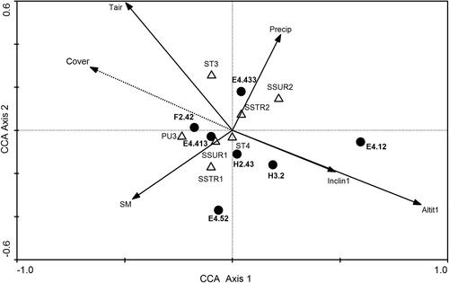
The relationships between HTs and environmental conditions are shown in Figure 2. In the CCA ordination biplot, only environmental variables (n = 12) that have statistically significant effects are displayed. We found that Outer Alpine Pinus mugo scrub (HT F2.42) had the densest canopy and occurred in the warmest sites with moist heterogeneous compact soils on relatively gentle slopes at lower altitudes. Rough hawkbit (Leontodon hispidus L.) pastures (HT E4.52), which had a relatively dense vegetation cover, grew at lower altitudes on a compact substrate with the wettest soils. The Southern rusty sedge grasslands (HT E4.413) grew in conditions very similar to those of P. mugo stands, while Cushion sedge carpets (HT E4.433) were characteristic of warmer sites with homogeneous soil of a loose texture and low water content. In addition, the sites with these HTs coincided with the highest amounts of precipitation. The Boreo-alpine calcicline snow-patch grassland and herb habitats (HT E4.12) had low vegetation cover and grew at higher altitudes on steeper sites and with abundant precipitation. Similar characteristics, though less steep slopes, were typical of Basic and ultra-basic inland cliffs (HT H3.2) and Calcareous screes (HT H2.43).

Figure 2. CCA ordination biplot based on seven HTs in relation to environmental factors (N = 12) exhibiting significant effects. The first axis explains 10.2% and the second axis 4.7% of the total variation in the data set. EUNIS codes and habitat names: E4.12_Boreo-alpine calcicline snow-patch grassland and herb habitats, E4.413_Southern rusty sedge grasslands, E4.433_Cushion sedge carpets, F2.42_Alpine Pinus mugo scrub, E4.52_ Rough hawkbit (Leontodon hispidus) pastures, H2.43_Fine calcareous screes, H3.2_Basic and ultra-basic inland cliffs. Abbreviations of environmental factors in Table 2.

During data exploration for regression analysis, some sampling sites were found to be spatial outliers and were, therefore, removed from the original dataset. The continuous variable average annual precipitation was removed from the analysis because it was collinear with average annual air temperature. Additionally, the categorical variables vegetation cover (collinear with altitude, inclination and average annual air temperature), rockiness (collinear with altitude, azimuth, inclination and average annual insolation), soil type (collinear with altitude and inclination) and pedocartographic units (collinear with azimuth, inclination and average annual air temperature) were also removed from the analysis. As a result, altitude, azimuth, inclination, average annual wind speed, average annual insolation, soil surface strength, soil surface structure, soil moisture and average annual air temperature were included in the regression analysis.

Environmental factors influencing the presence of the most abundant HTs in the highlands of the KS Alps

We analysed the influence of the environmental factors on the occurrence of the four most frequent HTs: Outer Alpine Pinus mugo scrub (F2.4), Southern rusty sedge grasslands (E4.413), Cushion sedge carpets (E4.433) and Fine calcareous screes (H2.43). The probability of the presence of Outer Alpine Pinus mugo scrub (HT F2.4) was best explained by orientation, inclination, average annual air temperature, soil surface structure and soil moisture (Table 3). It was found that the probability of the presence was highest at the sampling sites on west/northwest facing slopes. (Azim Estimated β ± SE: 0.0043 ± 0.0015, p = 0.004), and average air temperature (Tair Estimated β ± SE: 0.5429 ± 0.1644, p < 0.001). On the other hand, the probability of the presence decreased with increasing inclination (Inclin1 Estimated β ± SE: − 0.0258 ± 0.0123, p = 0.035). The probability of the presence was significantly lower at sites with a homogeneous soil surface (SSUR_homogeneous Estimated β ± SE: −0.8480 ± 0.3040, p = 0.013) in comparison to sites with heterogeneous soil (baseline category). We also found a significantly higher probability for the presence of HT F2.4 at sites with moist soil (SM_moist Estimated β ± SE: 0.8250 ± 0.2809, p = 0.003) as compared to sites with dry soil (baseline category), while sites with wet soil had no significant effect on the probability of the presence of this HT (SM_wet Estimated β ± SE: 1.0091 ± 0.5210, p = 0.053). The effects of environmental variables on the probability of presence are shown in Figure 3.

Figure 3. Predicted values from the best model (Table 3) for the effects of environmental factors on the probability of the presence of Outer Alpine Pinus mugo scrub (Eunis HT code F2.4, Natura 2000 code 4070*) in the KS Alps. In each plot, the unplotted variable is set at the mean value. Abbreviations of the explanatory variables: Dry, moist, wet – Soil moisture; SSUR1 – Soil surface structure (heterogeneous); SSUR2 – Soil surface structure (homogeneous).

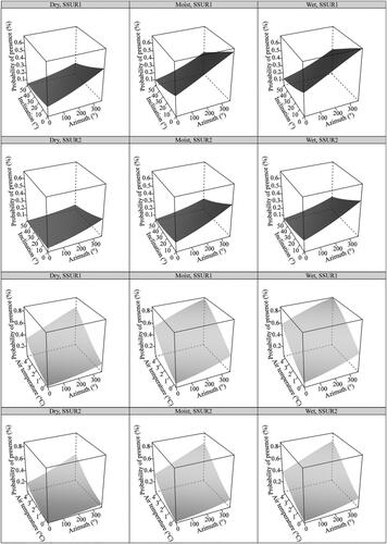
Table 3. Three best models predicting the probability of the presence of four HTs: Outer Alpine Pinus mugo scrub (Eunis code F2.4/Natura 2000 code 4070*), Southern rusty sedge grasslands (E4.413/6170), Cushion sedge carpets (E4.433/6170) and Fine calcareous screes (H2.43/8120), according to the AICc values.

Model structure	Df	AICc	ΔAICc	wi
Outer Alpine Pinus mugo scrub (F2.42/4070*)
Presence ∼ Azim + Inclin1 + Tair + SSUR + SM + 1|Mountain	8	256.70	0.00	0.57
Presence ∼ Azim + Inclin1 + Tair + SSTR + SSUR + SM + 1|Mountain	9	258.22	1.51	0.27
Presence ∼ Azim + Inclin1 + Insol1 + Tair + SSTR + SSUR + SM + 1|Mountain	10	259.95	3.25	0.11
Southern rusty sedge grasslands (E4.413/6170)
Presence ∼ Inclin1 + Tair + Wind + SSUR + 1|Mountain	6	261.76	0.00	0.45
Presence ∼ Inclin1 + Tair + Wind + SSUR + SM + 1|Mountain	8	262.35	0.60	0.33
Presence ∼ Azim + Inclin1 + Tair + Wind + SSUR + SM + 1|Mountain	9	264.06	2.30	0.14
Cushion sedge carpets (E4.433/6170)
Presence ∼ SSTR + SSUR + SM + 1|Mountain	6	284.97	0.00	0.54
Presence ∼ Inclin1 + SSTR + SSUR + SM + 1|Mountain	7	286.37	1.40	0.27
Presence ∼ Inclin1 + Wind + SSTR + SSUR + SM + 1|Mountain	8	287.98	3.01	0.12
Fine calcareous screes (H2.43/8120)
Presence ∼ Insol1 + Tair + SSUR + 1|Mountain	5	271.49	0.00	0.48
Presence ∼ Insol1 + Tair + SSUR + SM + 1|Mountain	7	272.93	1.44	0.23
Presence ∼ Inclin1 + Insol1 + Tair + SSUR + SM + 1|Mountain	8	273.64	2.15	0.16

Models are ordered from the most to the least appropriate. Abbreviations of the explanatory variables: Azim – Azimuth (°); Inclin1 – Inclination (°) (field data); Tair – Average annual air temperature (°C); SSUR – Soil surface structure; SM – Soil moisture; SSTR – Soil strength; Insol1 – Average annual insolation (kWh/m2) (uniform sky model); Wind – Average annual wind speed (m/s). Df – degrees of freedom; AICc – corrected Akaike information criterion; ΔAICc – AICc of the model subtracted by the AICc of the best model; w_i – Akaike weight.

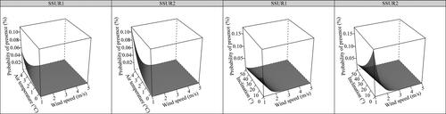
Inclination, average annual air temperature, wind speed and soil surface structure best explained (Table 3) the probability of the presence of Southern rusty sedge grasslands (HT E4.413). The probability of presence was found to increase significantly with increasing average annual wind speed (Wind Estimated β ± SE: 0.9290 ± 0.2778, p < 0.001) and average annual air temperature (Tair Estimated β ± SE: 0.8435 ± 0.2614, p = 0.001), and to decrease significantly with increasing inclination (Inclin1 Estimated β ± SE: −0.0371 ± 0.0176, p = 0.035). We found a significantly lower probability for the presence of HT E4.413 at sites with homogeneous soil (SSUR_homogeneous Estimated β ± SE: −2.6662 ± 0.5270, p < 0.001), as compared to sites with heterogeneous soil (baseline category). The effects of environmental variables on the probability of the presence of HT E4.413 are illustrated in Figure 4.

Figure 4. Predicted values from the best model (Table 3) for the effects of environmental factors on the probability of the presence of Southern rusty sedge grasslands (Eunis HT code E4.413, Natura 2000 habitat code 6170), in the KS Alps. In each plot, the unplotted variable is set at the mean value. Abbreviations of the explanatory variables: SSUR1 – Soil surface structure (heterogeneous); SSUR2 – Soil surface structure (homogeneous).

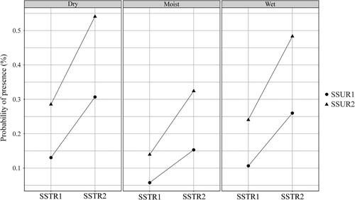
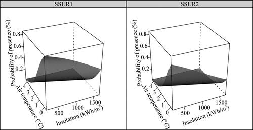
The probability of the presence of Cushion sedge carpets (HT E4.433) was best explained by soil strength, soil surface structure and soil moisture (Table 3). It was found that the probability of presence was significantly higher at sites with loose soil (SSTR_loose Estimated β ± SE: 1.0812 ± 0.3930, p = 0.006), as compared to sites with compact soil (baseline category), and significantly higher at sites with homogeneous soil (SSUR_homogeneous Estimated β ± SE: 0.9849 ± 0.2687, p < 0.001), as compared to sites with heterogeneous soil (baseline category). On the other hand, the probability of the presence of HT E4.433 was significantly lower at sites with moist soil (SM_moist Estimated β ± SE: −0.8977 ± 0.2507, p < 0.001), but not significantly different at sites with wet soil (SM_wet Estimated β ± SE: −0.2315 ± 0.6320, p = 0.714), compared to sites with dry soil (baseline category). Interaction plots showing the influence of environmental variables on the probability of the presence of this HT are illustrated in Figure 5.

Figure 5. Interaction plots of predicted values from the best model (Table 3) for the effects of environmental factors on the probability of the presence of Cushion sedge carpets (EUNIS HT code E4.433, Natura 2000 habitat code 6170) in the KS Alps. Abbreviations of the explanatory variables: Dry, moist, wet – Soil moisture; SSUR1 – Soil surface structure (heterogeneous); SSUR2 – Soil surface structure (homogeneous); SSTR1 – Soil strength (compact); SSTR2 – Soil strength (loose).

The model selection suggested that insolation, average annual air temperature and soil surface structure (Table 3) best explained the probability of the presence of Fine calcareous screes (HT H2.43). The probability decreased significantly with increasing insolation (Insol1 Estimated β ± SE: −0.0013 ± 0.0004, p = 0.002) and with increasing average annual air temperature (Tair β ± SE: −0.7579 ± 0.1986, p < 0.001). Additionally, we found a significantly lower probability of its presence at sites with a homogeneous soil surface (SSUR_homogeneous Estimated β ± SE: −1.1940 ± 0.3627, p = 0.001), as compared to sites with a heterogeneous soil surface (baseline category). The combined effect of these variables on the probability of the presence of this HT is shown in Figure 6.

Figure 6. Predicted values from the best model (Table 3) for the effects of environmental factors on the probability of the presence of Fine calcareous screes (EUNIS HT code H2.43, Natura 2000 habitat code 8120) in the KS Alps. Abbreviations of the explanatory variables: SSUR1 – Soil surface structure (heterogeneous); SSUR2 – Soil surface structure (homogeneous).

Discussion

Present results show that four typical alpine habitats, all Natura 2000 HTs, were most representative in the study area. Outer Alpine Pinus mugo scrub (EUNIS HT habitat code F2.42/Natura 2000 habitat code 4070*) dominates the slopes above the enclosed timberline and forms a coherent vegetation belt, known as the subalpine belt (Šibík et al. 2010). In the highlands of the KS Alps, this HT is represented by the Rhododendro hirsuti-Pinetum prostratae Zöttl 1951 association (Šilc and Čarni 2012), and the results of our analyses showed that the occurrence of Outer Alpine Pinus mugo scrubs was greatest on west-facing gentle slopes with higher average annual air temperatures. High-mountain systems have changed significantly in recent decades (Körner and Paulsen 2004; Palombo et al. 2014), and several studies have raised the possibility that the upward expansion of mountain pine at the European scale can be attributed to recent climate warming (Gehrig-Fasel et al. 2007; Švajda et al. 2011; Palombo et al. 2014). However, air temperature alone may not be the dominant factor determing P. mugo occurrence, as the direct influence of temperature can be masked by interactions with other factors, such as precipitation, cold-induced photoinhibition and plant-plant interactions (Harsch et al. 2009). Furthermore, we confirmed that soil water content is an important environmental factor influencing the presence of mountain pine growth (Palombo et al. 2014).

Alpine and subalpine calcareous grasslands (EUNIS habitat code E4.4, Natura 2000 code 6170) are species-rich habitats with many rare or endangered taxa listed in the Red List of Vascular Plants of Slovenia (Rules on the Inclusion of Endangered Plant and Animal Species in the Red List 2002), such as Chamorchis alpina (L.) Rich., Dianthus sternbergii Sieber ex F. N. Williams, Gentiana clusii E. P. Perrier & Songeon, Gymnadenia odoratissima (L.) Rich., Leontopodium alpinum Cass., Pseudorchis albida (L.) Á. Löve & D. Löve, Ranunculus alpestris L. and Saussurea alpina (L.) DC. (Surina 2005). Within this group, two HTs were identified in the field at the lower hierarchical level: Southern rusty sedge grasslands (HT E4.413; association Ranunculo hybridi-Caricetum sempervirentis), and the Cushion sedge carpets (HT 36.433), represented by the Gentiano terglouensis-Caricetum firmae association (Lippert 1987). Southern rusty sedge grasslands represent a widespread altimontane and subalpine plant HT in the KS Alps, with the greatest ecological valence among the HTs studied (Surina 2005). As shown in this study, the occurrence of this HT at altitudes above 1800 m was greatest on moderately steep slopes with a southern and southeastern exposure, and with higher temperatures and wind speed. In addition, soil surface structure also significantly influenced the presence of this HT; the occurrence of Southern rusty sedge grasslands was greatest at sites with heterogeneous soils. This HT and Alpine Pinus mugo scrub thrive at sites with very similar conditions.

Variables related to soil properties (e.g. soil surface structure, strength and moisture) were found to be very good predictors of the presence of Cushion sedge carpets (HT E4.433) in the study area. The occurrence of this HT was greatest at sites with homogeneous soil of loose texture and low water content, supporting published evidence (Kammer and Möhl 2002) that this HT, often fragmented in small patches of grassland dominated by Carex firma Host, grows on shallow, permeable soils on compact limestone or dolomite.

On steep slopes, the calciphilous Cushion sedge carpets meet the calcareous screes (HT H2.43/8120), replacing them where mobile screes become fixed (García-González 2008). The unstable calcareous screes are colonised by specialised plant communities that tolerate moderate substrate movement (Cannone and Gerdol 2003). Because this HT was prevalent at higher altitudes, longer insolation and lower average annual air temperature best predicted Cushion sedge carpets compared to the other HTs in our study.

The HTs examined in our study are rich in species and communities and in this way serve as reservoirs of biodiversity (García-González 2008). For many animal species that use these HTs for shelter and food, including those listed in Annex I in the Habitats Directive, e.g. butterflies (Pellissier et al. 2013; Leingärtner et al. 2014; Čelik et al. 2015), our results could help in the selection of suitable monitoring sites. On the other hand, some other taxa, e.g. harvestmen, do not show any association with HT distributions, but instead reveal specific ecological requirements (Novak et al. 2017).

We found that certain environmental factors, e.g. average annual air temperature, average annual insolation, inclination, soil surface structure and soil strength, were important predictors of most representative HTs, and thus useful for further refining of monitoring. Such monitoring should be implemented in highland ecosystems and habitats with conservation priority in Slovenia as well as throughout the EU (Miller and Kettunen 2007). The digitally modelled datasets efficiently represented the average values of selected geographical, physical, meteorological and paedological parameters, while the field research provided the only data on microhabitats. It is, therefore, useful to combine both datasets when available (Novak et al. 2017; Zellweger et al. 2019). Furthermore, the available field observations can be intersected with layers of different environmental data from optical and radar images, providing the opportunity to derive models for reliable predictions of all other locations of these HTs in the area (Minasny et al. 2019).

Our study extends the knowledge and understanding of the relationship between environmental conditions and the occurrence of highland HTs in the KS Alps, which probably concerns a great part of the Alpine highlands. Our results enable the interpretation of recent HT distribution patterns, based on which predictions can be made about possible future HT shifts and species extinctions (Brighenti et al. 2019; Rumpf et al. 2019; Schwager and Berg 2019). Such knowledge is essential to achieve credible, long-term conservation planning in alpine and subalpine vegetation communities.

Acknowledgements

We are grateful to Marko Goličnik, Saška Lipovšek, Bernarda Pačnik, Matej Pačnik, Ljuba Slana Novak, Jure Tostovršnik and Marija Verbuč for help with the field investigations. We are indebted to Michelle Gadpaille for valuable improvements to the language.

Disclosure statement

No potential conflict of interest was reported by the authors.

Additional information

Funding

The study was partly supported by the by the Slovenian Research Agency, core fundings P1-0403 and J7-1822.

References

- Aeschimann D, Lauber K, Moser DM, Theurillat J-P. 2004. Flora Alpina. Belin and Zanichelli: Haupt.
- [ARSO] Agencija Republike Slovenije za okolje. 2010. Ljubljana [accessed 2010 Nov 23]. http://meteo.arso.gov.si/met/sl/climate/maps/.
- Bartoń K. 2016. MuMIn: multi-model inference, version 1.15. [accessed 2020 Feb 15]. https://cran.r-project.org/web/packages.
- Bates D, Maechler M, Bolker B, Walker S, Christensen RHB, Singmann H, Dai B, Scheipl F, Grothendieck G, Green P, et al. 2020. Linear mixed-effects models using ‘Eigen’ and S4, version 1.1-23. [accessed 2020 Feb 15]. https://CRAN.R-project.org/package=lme4.
- Braun-Blanquet J. 1964. Pflanzensoziologie, Grundzüge der Vegetationskunde. (3. Auflage). Wien (Austria): Springer.
- Brighenti S, Tolotti M, Bruno MC, Wharton G, Pusch MT, Bertoldi W. 2019. Ecosystem shifts in alpine streams under glacier retreat and rock glacier thaw: a review. Sci Total Environ. 675:542–559.
- Burnham KP, Anderson DR. 2002. Model selection and multimodel inference: a practical information-theoretic approach. New York (NY): Springer.
- Cannone N, Gerdol R. 2003. Vegetation as an ecological indicator of surface instability in rock glaciers. Arct Antarct Alp Res. 35(3):384–390.2.0.CO;2]
- Casazza G, Zappa E, Mariotti MG, Médail F, Minuto L. 2008. Ecological and historical factors affecting distribution pattern and richness of endemic plant species: the case of the Maritime and Ligurian Alps hotspot. Divers Distrib. 14(1):47–58.
- Celarc B. 2004. Geološka zgradba [Geological structure]. In: Habjan V, Drab J, Poljanec A, Stritar A, editors. Kamniško-Savinjske Alpe: planinski vodnik [Kamnik–Savinja Alps: mounteneer guide]. Ljubljana (Slovenia): Planinska zveza Slovenije; p. 13–14.
- Chytrý M, Tichý L, Hennekens SM, Knollová I, Janssen JAM, Rodwell JS, Peterka T, Marcenò C, Landucci F, Danihelka J, et al. 2020. EUNIS habitat classification: expert system, characteristic species combinations and distribution maps of European habitats. Appl Veg Sci. 23(4):648–675.
- Čelik T, Bräu M, Bonelli S, Cerrato C, Vreš B, Balletto E, Stettmer C, Dolek M. 2015. Winter-green host-plants, litter quantity and vegetation structure are key determinants of habitat quality for Coenonympha oedippus in Europe. J Insect Conserv. 19(2):359–375.
- Devilliers P, Devilliers-Terschuren J. 1996. A classification of Palearctic habitats. Strasbourg (France): Council of Europe.
- Directive 1992/43/EEC of 21 May 1992 on the conservation of natural habitats and of wild fauna and flora H. 1992. OJEU. 206:7–50.
- Dirnböck T, Essl F, Rabitsch W. 2011. Disproportional risk for habitat loss of high-altitude endemic species under climate change. Global Change Biol. 17(2):990–996.
- [ESRI] Environmental Systems Research Institute. 2010. ArcGIS Desktop. Release 9.3. Redlands.
- EUR27. 2007. Natura 2000. Interpretation manual of European Union habitats. Strasbourg (France): European Commission DG Environment. Nature and Biodiversity.
- [FAO] Food and Agriculture Organisation. 2006. Guidelines for soil description. 4th ed.Rome (Italy): FAO.
- [FAO/IIASA/ISRIC/ISS-CAS/JRC] Food and Agriculture Organisation/International Institute for Applied Systems Analysis/World Soil Information/Institute of Soil Science, Chinese Academy of Sciences/Joint Research Centre of the European Commission. 2012. Harmonized World soil database (version 1.2). Rome (Italy): FAO, and Laxenburg; Austria: IIASA.
- Finch O-D, Löffler J. 2010. Indicators of species richness at the local scale in an alpine region: a comparative approach between plant and invertebrate taxa. Biodivers Conserv. 19(5):1341–1352.
- Gams I, Vrišer I, editors. 1998. Geografija Slovenije – priročnik [Geography of Slovenia – Manual]. Ljubljana (Slovenia): Slovenska matica.
- García-González R. 2008. Management of Natura 2000 habitats. 6170 Alpine and subalpine calcareous grasslands. Strasbourg (France): European Commission.
- Gehrig-Fasel J, Guisan A, Zimmermann NE. 2007. Tree line shifts in the Swiss Alps: climate change or land abandonment?J Veg Sci. 18(4):571–582.
- [GERK] Ministrstvo za kmetijstvo gozdarstvo in prehrano. 2010. Grafični in pisni podatki (shape, dbf) Pedološke karte in pedoloških profilov [Graphical and written data (shape, bdf) of the Pedological map and pedological profiles.] Ljubljana (Slovenia): GERK. [accessed 2020 Feb 15]. http://rkg.gov.si/GERK/.
- [GURS] Geodetska uprava Republike Slovenije. 2010. Digitalni model višin Slovenije 12,5x12,5 [Digital elevation model of Slovenia 12.5x12.5]. Ljubljana (Slovenia): GURS.
- Harsch MA, Hulme PE, McGlone MS, Duncan RP. 2009. Are treelines advancing? A global meta-analysis of treeline response to climate warming. Ecol Lett. 12(10):1040–1049.
- Hastie T. 2016. gam: generalized additive models. R package version 1.09. [accessed 2020 Feb 15]. http://CRAN.R-project.org/package=gam.
- Hegi G, Merxmüller H, Reisigl H. 1980. Alpska flora [Alpine flora]. Ljubljana (Slovenia): Državna založba Slovenie. Slovene.
- Hetrick WA, Rich PM, Barnes FJ, Weiss SB. 1993. GIS-based solar radiation flux models. ASPRS Tech Pap. 3:132–143.
- Holmquist JG, Jones JR, Schmidt-Gengenbach J, Pierotti LF, Love JP. 2011. Terrestrial and aquatic macroinvertebrate assemblages as a function of wetland type across a mountain landscape. Arct Antarct Alp Res. 43(4):568–584.
- Hurvich CM, Tsai CL. 1989. Regression and time series model selection in small samples. Biometrika. 76(2):297–307. .
- Jogan N, Kaligarič M, Leskovar I, Seliškar A, Dobravec J. 2004. Habitatni tipi Slovenije HTS 2004 tipologija [Habitat types of Slovenia, HTS 2004 typology]. Ljubljana (Slovenia): ARSO. Slovene.
- Jongman RHG, Braak CJF, Tongeren OFR. 1995. Data analysis in community and landscape ecology. Cambridge (UK): Cambridge University Press.
- Juvan N, Košir P, Marinšek A, Paušič A, Čarni A. 2013. Differentiation of the Piceetalia and Athyrio-Piceetalia forests in Slovenia. Tuexenia. 33:25–48.
- Kammer PM, Möhl A. 2002. Factors controlling species richness in alpine plant communities: an assessment of the importance of stress and disturbance. Arct Antarct Alp Res. 34(4):398–407.
- Kladnik D. 1981. Melišča v Kamniško–Savinjskih Alpah [Screes in the Kamnik–Savinja Alps]. In: Brinovec V, editor. Zbornik Referatov 12. zborovanja Slovenskih Geografov – Kranj, Bled [Proceedings of the 12th Meeting of Slovene Geographers – Kranj, Bled]. Ljubljana (Slovenia): Geografsko društvo Slovenije; p. 147–155.
- Körner C, Paulsen J. 2004. A world-wide study of high altitude treeline temperatures. J Biogeogr. 31(5):713–732.
- Kryštufek B, Klenovšek T, Amori G, Janžekovič F. 2015. Captured in ‘continental archipelago’: phylogenetic and environmental framework of cranial variation in the European snow vole. J Zool. 297(4):270–277.
- Lauber K, Wagner G. 2001. Flora Helvetica. Bern (Switzerland): Haupt.
- Leingärtner A, Krauss J, Steffan-Dewenter I. 2014. Species richness and trait composition of butterfly assemblages change along an altitudinal gradient. Oecologia. 175(2):613–623.
- Lepš J, Šmilauer P. 2003. Multivariate analysis of ecological data using CANOCO. Cambridge (UK): Cambridge University Press.
- Lippert W. 1987. Alpsko cvetje [Alpine flora]. Ljubljana (Slovenia): Cankarjeva založba.
- Martinčič A. 2008. Mahovna flora Smrekovškega pogorja (Kamniško-Savinjske Alpe, Slovenija) [Mossy flora of the Smrekovec Mts. (Kamnik–Savinja Alps, Slovenia)]. Hacquetia. 7(1):33–46.
- Martinčič A, Wraber T, Jogan N, Ravnik V, Podobnik A, Turk B, Vreš B. 1999. Mala flora Slovenije. [Slovenian flora]. Ljubljana (Slovenia): Tehniška založba Slovenije.
- Martinčič A, Wraber T, Jogan J, Podobnik A, Ravnik V, Turk B, Vreš B, Frajman B, Strgulc-Krajšek S, Trčak B, et al. 2007. Mala flora Slovenije. [Identification key for the Slovenian flora]. 4th ed. Ljubljana (Slovenia): Tehniška založba Slovenije.
- Marušič J, Jančič M, Zakotnik I, Kravanja N, Piano S. 1998. Krajine alpske regije, Regionalna razdelitev krajinskih tipov v Sloveniji. [Landscapes of the Alpine Region, Regional divison of landscape types in Slovenia]. Ljubljana (Slovenia): Ministry of the Environment and Spatial Planning.
- Mathar WP, Kämpf I, Kleinebecker T, Kuzmin I, Tolstikov A, Tupitsin S, Hölzel N. 2016. Floristic diversity of meadow steppes in the Western Siberian Plain: effects of abiotic site conditions, management and landscape structure. Biodivers Conserv. 25(12):2361–2379.
- Miller C, Kettunen M. 2007. Financing natura 2000: guidance handbook. Brussels (Belgium): European Commission—General Directorate for the Environment.
- Minasny B, Berglund Ö, Connolly J, Hedley C, de Vries F, Gimona A, Kempen B, Kidd D, Lilja H, Malone B. 2019. Digital mapping of peatlands – a critical review. Earth-Sci Rev. 196:102870.
- Moss D. 2008. EUNIS habitat classification—a guide for users. European Topic Centre on Biological Diversity. Luxembourg: European Environmental Agency. [accessed 2020 Apr 26]. http://bd.eionet.europa.eu.
- [Natura 2000]. Uredba o posebnih varstvenih območjih (območjih Natura 2000) [Ordinance on special protected areas (Natura 2000 areas)]. Official Gazette of the Republic of Slovenia 45/2004. [accessed 2020 Feb 15]. http://www.pisrs.si/Pis.web/pregledPredpisa?id=URED283.
- Novak T, Janžekovič F, Rak M, Ivajnšič D, Kozel P, Slana Novak L, Škornik S. 2017. Can highland habitat type distributions replace mapping of harvestman species?J Insect Conserv. 21(2):331–343. .
- Ogrin D, Plut D. 2009. Aplikativna fizična geografija Slovenije [Applied physical geography of Slovenia]. Ljubljana (Slovenia): Znanstvena založba Filozofske fakultete.
- Palombo C, Battipaglia G, Cherubini P, Chirici G, Garfì V, Lasserre B, Lombardi F, Marchetti M, Tognetti R. 2014. Warming-related growth responses at the southern limit distribution of mountain pine (Pinus mugo Turra subsp. Mugo). J Veg Sci. 25(2):571–583.
- Pellissier L, Alvarez N, Espíndola A, Pottier J, Dubuis A, Pradervand J-N, Guisan A. 2013. Phylogenetic alpha and beta diversities of butterfly communities correlate with climate in the western Swiss Alps. Ecography. 36(5):541–550.
- [PZS] Planinska zveza Slovenije. 1998. Grintovci mountaineer map. 1:25.000. Ljubljana (Slovenia): Planinska založba Planinske zveze Slovenije.
- R Development Core Team. 2018. R: A language and environment for statistical computing. Vienna: R Foundation for Statistical Computing. [accessed 2020 Feb 15]. https://www.R-project.org.
- Reutter BA, Helfer V, Hirzel AH, Vogel P. 2003. Modelling habitat-suitability using museum collections: an example with three sympatric Apodemus species from the Alp. J Biogeogr. 30(4):581–590.
- Rosbakh S, Römermann C, Poschlod P. 2015. Specific leaf area correlates with temperature: new evidence of trait variation at the population, species and community levels. Alp Botany. 125(2):79–86.
- Rules on the Inclusion of Endangered Plant and Animal Species in the Red list [Pravilnik o uvrstitvi ogroženih rastlinskih in živalskih vrst v rdeči seznam]. 2002. Priloga 1: Rdeči seznam praprotnic in semenk (Pteridophyta & Spematophyta) [Appendix 1: red list Pteridophyta and Spermatophyta]. Official Gazette of the Republic of Slovenia 82/2002:8893–8910.
- Rumpf SB, Hülber K, Wessely J, Willner W, Moser D, Gattringer A, Klonner G, Zimmermann NE, Dullinger S. 2019. Extinction debts and colonization credits of non-forest plants in the European Alps. Nat Commun. 10(1):4293. www.nature.com/naturecommunications.
- Sarkar D, Andrews F, Wright K, Klepeis N, Murrell P. 2017. lattice: Trellis Graphics for R, version 0.20-41. [accessed 2020 Feb 15]. https://CRAN.R-project.org/package=lattice.
- Scherrer D, Körner C. 2011. Topographically controlled thermal-habitat differentiation buffers alpine plant diversity against climate warming. J Biogeogr. 38(2):406–416.
- Schwager P, Berg C. 2019. Global warming threatens conservation status of alpine EU habitat types in the European Eastern Alps. Reg Environ Change. 19(8):2411–2421..
- Seliškar A. 1998. The habitat mapping in Slovenia – connection to the vegetation units. Working document, CORINE-PHARE project. Ljubljana (Slovenia): Institute of Biology at the Centre of Scientific Research of the Slovenian Academy of Sciences and Arts.
- Surina B. 2005. Subalpine and alpine vegetation of the Krn area in the Julian Alps. Scopolia. 57:1–222.
- Šibík J, Šibíková I, Kliment J. 2010. The subalpine Pinus mugo-communities of the Carpathians with a European perspective. Phytocoenologia. 40(2-3):155–188.
- Šilc U, Čarni A. 2012. Conspectus of vegetation syntaxa in Slovenia. Hacquetia. 11(1):113–164.
- Švajda J, Solár J, Janiga M, Buliak M. 2011. Dwarf pine (Pinus mugo) and selected abiotic habitat conditions in the Western Tatra Mountains. Mt Res Dev. 31(3):220–228.
- ter Braak CJF. 1986. Canonical correspondence analysis: a new eigenvector technique for multivariate direct gradient analysis. Ecology. 67(5):1167–1179. −
- ter Braak Ct, Šmilauer P. 2002. CANOCO reference manual and CanoDraw for Windows, User’s guide: Software for Canonical Community Ordination (version 4.5). Section on permutation methods. Ithaca (NY): Microcomputer Power.
- Tomaselli V, Dimopoulos P, Marangi C, Kallimanis AS, Adamo M, Tarantino C, Panitsa M, Terzi M, Veronico G, Lovergine F, et al. 2013. Translating land cover/land use classifications to habitat taxonomies for landscape monitoring: a Mediterranean assessment. Landscape Ecol. 28(5):905–930.
- Väre H, Lampinen R, Humphries C, Williams P. 2003. Taxonomic diversity of vascular plants in the European alpine areas. In: Nagy L, Grabherr G, Körner C, Thompson DBA, editors. Alpine biodiversity in Europe. Berlin (Germany): Springer; p. 133–148.
- Wickham H, Chang W, Henry L, Pedersen TL, Takahashi K, Wilke C, Woo K, Yutani H, Dunnington D, Rstudio. 2020. ggplot2: create elegant data visualisations using the grammar of graphics, version 3.3.0. [accessed 2020 Feb 15]. https://CRAN.R-project.org/package=ggplot2.
- Wraber T. 2006. Dvakrat sto alpskih rastlin na Slovenskem [Two times hundred plants in Slovenia]. Ljubljana (Slovenia): Prešernova družba.
- Zellweger F, De Frenne P, Lenoir J, Rocchini D, Coomes D. 2019. Advances in microclimate ecology arising from remote sensing. Trends Ecol Evol. 34(4):327–341.
- Zuur AF, Hilbe JM, Ieno EN. 2013. A beginner’s guide to GLM and GLMM with R. Newburgh (NY): Highland Statistics.
- Zuur AF, Ieno EN. 2016. A protocol for conducting and presenting results of regression-type analyses. Methods Ecol Evol. 7(6):636–645.
- Zuur AF, Ienom EN, Walkerm NJ, Savalievm AA, Smith GM. 2009. Mixed effect models and extensions in ecology with R. Berlin (Germany): Springer.