Relevance of inhomogeneous–anisotropic models of human cortical bone: a tibia study using the finite element method

ABSTRACT

Cortical bone is an inhomogeneous and anisotropic tissue subjected to large loads during typical daily activities. While studies assuming isotropic material properties are frequent, anisotropy and inhomogeneity of cortical bone have been rarely taken into account. Moreover, the question, whether an assumption of anisotropy and inhomogeneity has an impact in the mechanical analysis of cortical bone, has not been explored in the literature. This study explores the relevance of anisotropy in human cortical bone. The cortical bone model has been divided into six radial regions and a different set of orthotropic material properties has been assigned to each region. This inhomogeneous and anisotropic elastic tibia model has been compared with a corresponding isotropic model under various loading modes using the finite element method. In particular, the variation in the maximum von Mises stress and strain values has been observed along the bone axis. We have observed that the isotropic model may overestimate the maximum von Mises strain up to 15% under pure compression and underestimate up to 50% under pure torsion relative to the inhomogeneous–anisotropic model. Our results suggest that consideration of anisotropy and inhomogeneity of the bone may make a significant difference in the predicted maximum von Mises strain values, which can be important for strain-based damage accumulation studies and fracture risk evaluation.

KEYWORDS:

• Cortical bone
• anisotropy
• inhomogeneity
• finite element
• von Mises strain
• tibia

Introduction

Long bones, such as the femur and the tibia, can sustain significant loads during daily activities, increasing to extreme levels under conditions of exercise and strenuous work.[1] The underlying mechanical properties of the hard tissues enable these structures to perform their intended function. Nevertheless, it is well known that the mechanical properties of bones depend on several factors such as age, diet, mobility and disease,[2–4] which could impact their performance.

Cortical bone is known to be inhomogeneous and anisotropic. While studies assuming isotropy are frequent, the anisotropic nature of the cortical bone has been rarely taken into account. Moreover, the question, whether an assumption of anisotropy and inhomogeneity has a large impact in the mechanical analysis of cortical bone, remains largely unanswered in literature. In this work, we have tried to provide an answer to this question.

To our knowledge, only two studies have implemented inhomogeneous and anisotropic whole bone models in the literature,[5,6] both of which concerned the femur. Both studies have utilized imaging data to obtain the density distribution in the bone, and relied on the derivation of orthotropic elastic constants from available empirical relations between bone density and material properties. However, while applicable to cancellous bone, the orthotropic elastic constants are known not to correlate well with the bone density in cortical bone.[7] It has been pointed out that the outcome of such studies is highly dependent on the chosen density–modulus relationship.[6] Furthermore, the study by Peng et al. also has been criticized for improper selection of the anisotropy frame.[6,8] Consequently, a realistic mechanical analysis of cortical bone, where anisotropy and inhomogeneity are properly taken into account, seems to be missing in the literature. Furthermore, the question whether these factors make a significant difference over an isotropic–homogeneous model has not been explored.

In this work, we have compared an inhomogeneous–anisotropic model of tibial cortical bone to a corresponding isotropic model using the ANSYS (Swanson Inc., Houston, PA, USA) finite element (FE) package with the intent to explore whether material property assumptions make a significant difference in the mechanical analysis of bone. Material properties, obtained directly through mechanical experimentation for different radial parts of the bone,[9] have been utilized in order to avoid less realistic material properties derived from density–modulus relationships. The variation in orthotropy axes throughout the tissue has been accounted for, by considering the natural structure of cortical bone. The variation in the maximum von Mises stress and strain values has been observed along the bone axis. The results regarding the von Mises strain distribution in the bone have been of particular interest since this significant quantity has been mostly omitted in the previous studies.

As certain mechanical quantities are hard or impossible to measure through experimentation, the constraints associated with experimental studies are the very reason why many researchers turn to powerful numerical tools such as the finite element method (FEM) to study tissue mechanics. Over the years, finite element analysis (FEA) has become a valuable tool to the researchers in the study of bone biomechanics. With appropriate FEA attributes and a proper model, FEA provides good predictions about the modelled phenomenon and has been validated numerous times in the biomechanics literature for a variety of situations. (See Mackerle for a literature survey of FEA used in orthopaedics and for discussion of validation.[10])

The first FE studies analysing bones assumed the tissue to be linearly elastic, isotropic and homogeneous. Long bones analysed under these assumptions, either as partial or whole structures, were mainly studied for the evaluation of strength.[11,12] Tibia, along with femur, has been frequently the subject of such strength studies. In one of the first studies, Cook et al. investigated the stress distribution in the proximal tibia in cases of tibia vara.[11] Metha and Rajani studied the effect of varying material properties on bone stresses in human tibia and fibula.[13] Tibial models, involving the whole bone or only the proximal tibia, with or without the intramedullary canal, were also studied in models where the bone was assumed to be transversely isotropic.[14]

In recent studies, the anisotropic nature of the tibia was taken into account by dividing the bone into three parts (distal and proximal parts, and the shaft) and assigning each part a different set of elastic properties. Gefen conducted such a study where stresses induced in cases of imbalanced joint-muscle loading, muscular weakness during intensive physical exercise and exposure to micro-gravity during space flight were analysed.[15] In a study by Limbert et al., the stiffness of tibia with torsional deformities was compared with the stiffness of normal tibia. This study utilized children tibia where the cortical part of the bone was considered homogenous and transversely isotropic, and the trabecular bone in the distal and proximal parts was assumed to be inhomogeneous and isotropic.[16] Similarly, Ionescu et al. simulated distal and proximal trabecular bones as inhomogeneous and transversely isotropic, and the cortical bone as orthotropic to study the stresses induced in the epiphysis.[17]

In the current work, we have tried to analyse the relevance of anisotropy and inhomogeneity in the mechanical analysis of cortical bone using a tibia example. Experimentally determined material properties have been taken from the literature and assigned to appropriate regions in the cortical tibia model which is then analysed via the FE method.

Materials and methods

Model formation

The utilized model was obtained by processing computed tomography (CT) images of a healthy male human tibia. Transverse CT (Toshiba Asteion, TSX-021B) images were taken at intervals of 1 mm. The contours of the cortical surfaces and intramedullary canals were manually drawn on each slice picture (Figure 1), using the CATIA solid modelling package (Dassault Systèmes, France). The contours were combined to form the cortical and intramedullary surfaces of the bone. The solid model was obtained by filling the gap between these surfaces (Figure 2). Bone marrow does not have any significant effect on the bone strength [18] and was omitted from the model.

Figure 1. CT pictures and bone contours of the tibia.

Figure 2. (From left to right) posterior, anterior, lateral and medial views of the tibia.

The diaphysis was divided into six radial regions (Figure 3) in order to apply the inhomogeneous and anisotropic properties as described by Knets et al. and Pfafrod et al.[9,19]

Figure 3. Six material regions of cortical tibia and the reference axes illustrated for one material region (Region 4).

Material properties

The six regions created during the model formation are used to impose anisotropy and inhomogeneity to the bone model. An orthotropy frame was defined at the cortical midpoint of each of these regions and it was assumed to be invariant within the region. In each region, the first local axis of the material frame (x₁ in Figure 3) was assumed to be perpendicular to the bone surface at the cortical midpoint. The second and third axes (x₂ and x₃ in Figure 3) were selected to point in the circumferential and axial directions, respectively. The tibia model was analysed in three distinct studies, each making use of a distinct strategy for the assignment of material properties to these regions.

In Study 1, the six separate regions were assigned unique orthotropic material properties in an attempt to account for the anisotropic and inhomogeneous nature of the diaphysis (Table 1). Moreover, as described earlier, orthotropy frames differed from one region to the other to account for the anisotropy of the diaphysis. In Study 2, each region was assigned the same orthotropic material properties, although with different axes orientations. The material properties were obtained by averaging the values of elastic constants over the regions (Table 1) and assigned to all regions with differing orthotropy frames. It should be clear that Study 1 assumes an inhomogeneous and anisotropic diaphysis while Study 2 regards the diaphysis as anisotropic but homogeneous.

Table 1. Young's moduli (E in GPa), Poisson's ratios (ν) and shear modulus (G in GPa) values of six cortical bone regions in human tibia and the related average values.[9]

		Cortical bone (diaphysis) material constants
Model	Explanation	E1	E2	E3	ν12	ν13	ν23	G12	G13	G23
	Region 1	7.54	8.23	19.6	0.55	0.12	0.12	2.21	3.39	5.00
Study 1 (anisotropic–inhomogeneous)	Region 2	6.16	8.13	18.5	0.46	0.10	0.13	2.53	3.43	5.18
	Region 3	7.83	9.18	17.5	0.49	0.14	0.16	2.40	3.94	5.23
	Region 4	6.15	8.21	16.0	0.43	0.12	0.15	2.29	3.00	4.41
	Region 5	7.60	9.48	18.4	0.49	0.14	0.16	2.69	4.53	5.12
	Region 6	6.13	7.80	20.2	0.51	0.09	0.12	2.45	3.06	4.60
Study 2 (anisotropic–homogeneous)	Region average	6.91	8.51	18.4	0.49	0.12	0.14	2.41	3.56	4.91
Study 3 (isotropic–homogeneous)	Loadings 1–3			E = 18.4		ν = 0.13
	Loading 2					ν = 0.13			G = 4.24

In Study 3, the entire diaphysis was assumed to be isotropic and homogeneous. For a proper comparison with the anisotropic models of Studies 1 and 2, a set of equivalent isotropic properties had to be generated from the available set of orthotropic properties, which necessitates some further clarification.

An isotropic elastic medium has only two independent constants. Hence, we had to choose two constants out of the nine available orthotropic constants in order to generate an appropriate isotropic model to be compared with the related orthotropic model. Under different loading modes, certain strain components will be larger than the others in the material. For a fair comparison of strains in an orthotropic model and an isotropic model, those material constants, that affect the dominant strain components the most, must be of comparable magnitude in both models. Consequently, the independent constants of the isotropic model were chosen according to the loading mode applied to the model. (Each model was studied under three different loading modes as explained in detail in the next subsection.) In the presence of axial loading, the average axial Young's modulus (E₃) and the average of the Poisson's ratios associated with the x₁–x₂ plane (v₁₃ and v₂₃) were taken as independent isotropic constants in an effort to have axial strains comparable to those in the orthotropic models. This resulted to a Young's modulus of E = 18 MPa and a Poisson's ratio of v = 0.13. Similarly, in case of pure torsional loading, where shear strains are dominant, we have taken again the average Poisson's ratios associated with the x₁–x₂ plane (v₁₃ and v₂₃) and the average of the shear moduli associated with the same plane (G₁₃ and G₂₃) as the independent isotropic constants. The resulting values for Poisson's ratio and shear modulus were v = 0.13 and G = 4.24 MPa, respectively (Table 1).

The material properties assigned to the epiphyses (where trabecular bone is abundant) differed from those assigned to the diaphysis (where bone is cortical). In all studies, the epiphyses were considered homogeneous due to the difficulties associated with quantification of localized material inhomogeneity. The anisotropy in this region was partially accounted in Studies 1 and 2, by adopting an orthotropic model from the literature [17] involving six independent elastic constants. This model is close to a transversely isotropic one (that has five independent constants) and sometimes used to study the mechanics of fibre composites. In Study 3, the axial Young's modulus (E₃) and the Poisson's ratio of the x₁–x₂ plane (v₁₃) were used for E and v values of isotropic epiphyses, respectively (Table 2).

Table 2. Elastic moduli (GPa) and Poisson's ratio values of the epiphyses in human tibia (adopted from [17]).

	Trabecular bone (epiphyses) material constants
Model	E1 = E2	E3	ν12	ν13 = ν23	G12	G13 = G23
Studies 1 and 2	4.48	9.64	0.35	0.12	1.41	1.28
Study 3		E = 9.64	ν = 0.35

Boundary conditions, finite element analysis

In all studies, the tibia was analysed under three different loading conditions: axial compression (Loading 1), torsion (Loading 2) and a combination of axial compression and torsion (Loading 3).

In all analyses, the tibia model was fixed to the ground at its distal end. For axial loading, a force of 2450 N was applied to the tibia as proposed in the literature.[14,20] The load was applied with a 60% and 40% distribution (Figure 4), namely 1470 and 980 N, on the medial and lateral condyles of the tibia, respectively.[21] In torsional loading, a torque of 20 Nm was applied along the bone axis.[22,23] For the third analysis, a combination of axial compression and torsion was applied to the bone using the force and torque values mentioned earlier.

Figure 4. Boundary conditions.

The anatomically accurate three-dimensional (3D) solid model of the tibia was transferred into ANSYS FE software and meshed with tetrahedral elements. The entire mesh of the human tibia consisted of 752,386 tetrahedrons with 1,074,905 nodes (Figure 5). The FE analyses were performed using the same software package.

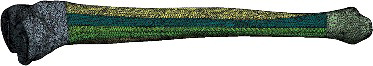
Figure 5. The finite element mesh of the tibia model with different material regions shown in different colouring.

Results and discussion

Failure criteria for cortical (and also trabecular) bone are typically based on von Mises stress or strain.[24] Hence, in this study, the distribution of von Mises stress and strain in the cortical bone was investigated. Rather than concentrating on individual points, where stress or strain takes a maximum value, we determined the maximum value of von Mises stress and strain at each cross section of the bone by post-processing the 3D FE results (Figure 6), and observed how these quantities evolved along the bone axis. Thus, we hoped to capture any general trends in the stress and strain values valid for the entire diaphysis. Observations were made only on the results of the diaphysis (whose position is indicated with vertical bars in the tibia sketch included in Figures 7–12).

Figure 6. Sample 3D result of von Mises stress distribution (MPa) on anterior (left) and posterior (right) sides of tibia.

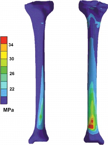
Figure 7. Maximum von Mises stress distribution under compressive loading.

Figure 8. Maximum von Mises stress distribution under torsional loading.

Figure 9. Maximum von Mises stress distribution under combined compressive and torsional loadings.

Figure 10. Maximum von Mises strain distribution under compressive loading.

Figure 11. Maximum von Mises strain distribution under torsional loading.

Figure 12. Maximum von Mises strain distribution under compressive and torsional loadings.

Variation in material properties is known to have a stronger effect on strain values than on stress values. In agreement with that, the resulting stress values for the inhomogeneous–anisotropic models (Study 1) and homogeneous–anisotropic (Study 2) models were not significantly different from those obtained for the homogeneous–isotropic model in all three loading modes. In particular, under pure compression and combined compression-torsion, all applied material models produced von Mises stress results that differ slightly (Figures 7 and 9). The difference was more notable under pure torsion, where the isotropic model (Study 3) overestimated the maximum von Mises stress as compared to the anisotropic and inhomogeneous–anisotropic models (Figure 8). Nevertheless, the difference was typically less than 8%, which is not significant given the variability of such biomechanical models.

A more notable difference was observed for the calculated maximum von Mises strain values for all material models. Under pure compression, the isotropic model overestimated the maximum von Mises strain by up to 15% as compared to the anisotropic and inhomogeneous–anisotropic models (Figure 10). Under pure torsion, the difference was more significant, with the isotropic model underestimating the strain values by up to 50% at certain cross sections (Figure 11) when compared to both anisotropic and inhomogeneous–anisotropic models. The observed difference was smaller between different material models when compression and torsion loads were combined. In this loading mode, the strain values in the isotropic model were overestimated in certain cross sections and underestimated in others when compared to anisotropic and inhomogeneous–anisotropic models. The difference in the numerical values was observed to be as high as 30% at certain cross sections (Figure 12).

Studies indicate that strain-based failure criteria are more accurate than stress-based ones, particularly for trabecular bone [25,26] and also for cortical bone.[27] Moreover, studies analysing damage accumulation in cortical bone usually correlate modulus reduction to strain.[28–30] Hence, in order to assess the damage accumulation in the bone and the associated fracture risk realistically, it is vital that the strain distribution is predicted accurately in simulation studies. Our results indicate that the assumption of an isotropic cortical bone might be inadequate to obtain a reasonable prediction for strain distribution in the bone. Compared to anisotropic material properties, prediction of isotropic properties requires significantly less experimentation, and isotropic models are simpler to implement within the FEM. Yet, an anisotropic model, no matter what complexities it brings, seems to be a necessary ingredient for a proper mechanical analysis of cortical bone.

Our study revealed that the difference in the strain results was minimal between homogeneous–anisotropic and inhomogeneous–anisotropic models. Yet, we believe that it would be premature to label inhomogeneity as insignificant based on this observation. The inhomogeneity issue can be tackled at very different levels in such situations. For example, if proper experimental material property data are available, the bone can be subdivided into a higher number of material regions in the transverse plane and even along the bone axis. The outcome of such an analysis may lead to different observations about the significance of inhomogeneity.

We have applied realistic force boundary conditions on the proximal part of the tibia in Loading 1 and 3 cases. Under different physiological conditions, the actual force on the bone may vary in magnitude and distribution. Note that the diaphysis of the bone is relatively far away from the anatomical force boundary. According to St. Venant's principle, away from the force boundary, stresses and strains are affected more from the magnitude of the total force and much less from its distribution. Since we have made observation only on the diaphysis and not epiphyses of the bone, we do not expect our results to change much in case of a different force distribution on the tibial plateau. Since the analysis is linear, a change in the magnitude of the total force will cause a proportional change in the observed stress and strain values. Hence, the difference that we have observed between isotropic and anisotropic cases will remain even if the force magnitude changes. Note that, in this study, we have evaluated the results qualitatively instead of paying much attention to the numerical values of the observed quantities.

This study encompassed the analysis of a single tibial model. Analyses of other tibia models, even with the same set of material properties, may lead to stress and strain values of differing magnitude since the bone mass and bone size may change significantly from one person to the other. However, the shape variability of the (healthy) tibia from one person to the other is relatively small, and a comparison of isotropic and inhomogeneous–anisotropic models is very likely to lead to similar conclusions even when multiple models are analysed.

A real bone is likely to possess a smooth variation in material properties. On the other hand, in our analysis, we have divided the cortical bone in six material regions with clear boundaries to approximate the bone inhomogeneity. Such a division might lead to unrealistic results (such as unrealistically spiked stress and strain values) at the interfaces of different material regions. In this work, our results do not suffer from this potential artifact since the reported maximum values of stress and strain were not observed at the material interfaces.

Our results indicate the importance of anisotropy; yet, determining the anisotropy and inhomogeneity in cortical bone is not a straightforward experimental task. Attempts have been made to correlate anisotropic material properties of trabecular and cortical bone to the bone density.[31–33] Combined ultrasound and CT studies revealed a good correlation between the moduli (measured along the three orthogonal axes) and the apparent density in the trabecular bone. This is expected since apparent density can vary several folds within the trabecular bone, allowing a proper correlation with elastic constants. Since density varies in a relatively small range in cortical bone, a correlation between the moduli and the density is not as effective as in trabecular bone.[7] If anisotropic elastic properties (along with the anisotropy frame) can be determined in vivo in an efficient way, then simulations involving anisotropic models can be more preferable to researchers.

Conclusions

In this study, an attempt was made to predict the maximum von Mises stress and strain value at each cross section of a typical human tibia and observe their variation along the inhomogeneous and anisotropic diaphysis of the bone. It was observed that anisotropic models can predict different strain distributions in cortical bone. In particular, inhomogeneous–anisotropic and homogeneous–anisotropic models predicted significantly different von Mises strain values when compared to the isotropic model under axial and torsional loadings. Our results indicate that the anisotropy of the cortical bone has to be taken into account to obtain a reasonable prediction for strain distribution in the bone, which could be important in bone strength studies.

Disclosure statement

No potential conflict of interest was reported by the authors.

References

- Huston RL. Principles of biomechanics. Boca Raton (FL): CRC Press; 2009.
- Mow VC, Huiskes R. Basic orthopaedic biomechanics & mechano-biology. 3rd ed. Philadelphia (PA): Lippincott; 2005.
- Ozkaya N, Nordin M. Fundamentals of biomechanics: equilibrium, motion, and deformation. 2nd ed. New York (NY): Springer; 1999.
- Wang X, Nyman JS, Dong X, et al. Fundamental biomechanics in bone tissue engineering. San Rafael (CA): Morgan & Claypool; 2010.
- Peng L, Bai J, Zeng X, et al. Comparison of isotropic and orthotropic material property assignments on femoral finite element models under two loading conditions. Med Eng Phys. 2006;28:227–233.
- Yang H, Ma X, Guo T. Some factors that affect the comparison between isotropic and orthotropic inhomogeneous finite element material models of femur. Med Eng Phys. 2010;32:553–560.
- Rho JY, Hobatho MC, Ashman RB. Relations of mechanical properties to density and CT numbers in human bone. Med Eng Phys. 1995;17:347–355.
- Baca V, Horak Z. Comparison of isotropic and orthotropic material property assignments on femoral finite element models under two loading conditions. Med Eng Phys. 2007;29:935.
- Knets IV, Saulgozis YZ, Yanson KA. Deformability and strength of compact bone tissue during tensioning. Polym Mech. 1974;10:419–423.
- Mackerle J. Finite element modeling and simulations in orthopedics: a bibliography 1998–2005. Comput Methods Biomech Biomed Eng. 2006;9:149–199.
- Cook S, Lavernia C, Burke S, et al. A biomechanical analysis of the etiology of tibia vara. J Pediatr Orthoped. 1983;3:449–454.
- Little RB, Wevers HW, Siu D, et al. A three-dimensional finite element analysis of the upper tibia. J Biomech Eng. 1986;108:111–119.
- Mehta BV, Rajani S. Finite element analysis of the human tibia. Trans Biomed Health. 1995;2:309–316.
- Müller-Karger CM, Gonzalez C, Aliabadi MH, et al. Three dimensional BEM and FEM stress analysis of the human tibia under patholological conditions. Comput Model Eng Sci. 2001;2:1–13.
- Gefen A. Consequences of imbalanced joint-muscle loading of the femur and tibia: from bone cracking to bone loss. In: Leder RS, editor. 25th Annual International Conference of the IEEE: Engineering in Medicine and Biology Society. Proceedings; 2003 Sep 17–21; Cancun (Mexico): IEEE; 2003; p. 1827–1830.
- Limbert G, Estivalezes E, Hobatho MC, et al. In vivo determination of homogenised mechanical characteristics of human tibia: application to the study of tibial torsion in vivo. Clin Biomech (Bristol, Avon). 1998;13:473–479.
- Ionesco I, Conway T, Schonning A, et al. Solid modeling and static finite element analysis of the human tibia. ASME Summer Bioengineering Conference. Proceedings; 2003 Jun 25–29; Key Biscayne (FL): ASME; 2003.
- Kasraa M, Grynpasb MD. On shear properties of trabecular bone under torsional loading: effects of bone marrow and strain rate. J Biomech. 2007;40:2898–2903.
- Pfafrod GO, Slutskii LI, Moorlat PA, et al. Evaluation of some deformation and strength characteristics of compact bone tissue according to the data of a biochemical study. Polym Mech. 1976;12:934–942.
- Harrington I. A bioengineering analysis of force actions at the knee in normal and pathological gait. Biomed Eng. 1976;11:167–172.
- Duda GN, Mandruzzato F, Heller M, et al. Mechanical boundary conditions of fracture healing: borderline indications in the treatment of unreamed tibial nailing. J Biomech. 2001;34:639–650.
- Bellchamber T, van den Bogert AJ. Contributions of proximal and distal moments to axial tibial rotation during walking and running. J Biomech. 2000;33:1397–1403.
- Hull ML, Johnson C. Axial rotation of the lower limb under torsional loading: I. Static and dynamic measurements in vivo. In: Johnson RJ, Mote CD, Binet M-H, editors. Skiing Trauma and Safety: Seventh International Symposium. Proceedings; 1987 May 11–15; Chamonix. Philadelphia (PA): ASTM International; 1989. p. 277–290.
- Nalla RK, Stolken JS, Kinney JH, et al. Fracture in human cortical bone: local fracture criteria and toughening mechanisms. J Biomech. 2005;38:1517–1525.
- Keaveny TM, Morgan EF, Niebur GL, et al. Biomechanics of trabecular bone. Annu Rev Biomed Eng. 2001;3:307–333.
- Sanyal A, Gupta A, Bayraktar HH, et al. Shear strength behavior of human trabecular bone. J Biomech. 2012;45:2513–2519.
- Nalla RK, Kinney JH, Ritchie RO. Mechanistic fracture criteria for the failure of human cortical bone. Nat Mater. 2003;2:164–168.
- Morgan EF, Lee JJ, Keaveny TM. Sensitivity of multiple damage parameters to compressive overload in cortical bone. J Biomech Eng. 2005;127:557–562.
- Nyman JS, Leng H, Neil Dong X, et al. Differences in the mechanical behavior of cortical bone between compression and tension when subjected to progressive loading. J Mech Behav Biomed Mater. 2009;2:613–619.
- Luo Q, Leng H, Acuna R, et al. Constitutive relationship of tissue behavior with damage accumulation of human cortical bone. J Biomech. 2010;43:2356–2361.
- Keyak JH, Rossi SA, Jones KA, et al. Prediction of femoral fracture load using automated finite element modeling. J Biomech. 1998;31:125–133.
- Chen G, Schmutz B, Epari D, et al. A new approach for assigning bone material properties from CT images into finite element models. J Biomech. 2010;43:1011–1015.
- Teo J, Si-Hoe K, Keh J, et al. Correlation of cancellous bone microarchitectural parameters from micro CT to CT number and bone mechanical properties. Mat Sci Eng C-Biomim. 2007;27:333–339.