Prediction of protein secondary structure based on deep residual convolutional neural network

Abstract

Proteins play a vital role in organisms, which suggests that in-depth study of the function of proteins is helpful to the application of proteins in a more accurate and effective way. Accordingly, protein structure will become the focus of discussion and research for a long time. In order to fully extract the effective information from the protein structure and improve the classification accuracy of the protein secondary sequence, a deep residual network model using different residual units was proposed to predict the secondary structure. This algorithm uses sliding window method to represent amino acid sequences and combines the powerful feature extraction ability of resent network. In this paper, the parameters of the neural network are debugged through experiments, and then the extracted features are classified and verified. The experimental results on CASP9, CASP10, CASP11 and CASP12 data sets imply that the improved deep residual network model based on different residual units can express amino acid sequences more accurately, which is more superior than existing methods.

Keywords:

• Convolutional neural networks
• protein
• residual network
• classification
• optimization

Introduction

The secondary structure of the protein defines the local conformation of the peptide main chain, which helps to identify the protein functional domains and guide the reasonable design of site-directed mutagenesis experiments [1]. Protein secondary structure can also be used for protein sequence alignment [2,3] and protein function prediction [4–6]. The prediction of protein secondary structure is usually divided into eight classes of H, G, I, E, B, T, S and ‘-’ Q8 accuracy. Then, the accuracy of these 8 classes is converted into three classifications of C (coil), H (helix) and E (strand), which is called Q3 accuracy [7]. With the in-depth study of protein structure [6], the Q3 accuracy of protein structure ranges from 69.7% of PHD server [8] to 76.5% of PSIPRED [9]. From the integrated neural network (SPINE) proposed by Faraggi et al. [10] to Hefferman et al. [11] using long and short memory neural networks and bidirectional recurrent neural networks (SPIDER2), prediction accuracies of up to 82% have been achieved. A large number of previous studies suggest that researchers usually predict the secondary structure of proteins by two stages. First of all, the protein sequences of different lengths are expressed as vectors by feature extraction, and then the feature vectors are input into a classification algorithm for prediction.

For protein sequence feature extraction, some scholars have proposed mathematical statistics and spectrum analysis methods, such as amino acid composition characteristics (AAC) [12], pseudo-amino acid composition [13] and position-specific scoring matrix (PSSM) [9], etc. Among them, the PSSM feature can fully take into account the position information of amino acids in the sequence and the interaction between amino acids, because it takes into account the composition information of the protein sequence, so in a previous research, a better prediction effect has been obtained [14]. In addition, in order to better represent the characteristic information of other amino acids near the target amino acid, a sliding window with a specified unit length is selected to extract the feature. The influence of input feature sliding window size on prediction accuracy is analyzed in reference [15]. Accordingly, this paper selects a fixed-size window, with each target amino acid as the centre, and extracts the characteristics of all the amino acids in the window by sliding along the sequence.

For the purpose of classification prediction, numerous researchers combine PSSM with deep learning algorithm [16,17] in order to achieve better prediction results. For example, Wang et al. [18] propose a DeepCNF algorithm to predict the protein secondary structure using the deep convolution neural network (CNN) with conditional random fields, and achieve 68.3% Q8 accuracy and 82.3% Q3 accuracy on the benchmark CB513 data set. Li and Yu [19] use a multi-scale convolution layer, followed by a three-layer stacked two-way loop layer, achieving a Q8 accuracy of 69.7% on the same test data set. Busia and Jaitly [20] introduce multi-scale convolution layers and residual networks to capture interactions in different ranges. Heffernan et al. [21] adopt long-term and short-term memory bi-directional cyclic neural networks (LSTM-bRNN) for iterative training, and achieved 84% Q3 accuracy on the data sets used in their previous study [22]. Christian et al. [23] achieve protein sequence prediction accuracy up to 81.5% by combining the hidden Markov model with neural network. The PSRSM template proposed by Ma et al. [24], through the method of partition and semi random subspace method (PSRSM), predicts the three classes of protein data according to the principle of majority voting, and the accuracy of Q3 is improved to 85.89%. It is worth noting that current deep learning methods further introduce different deep architectural innovations, including residual networks [25,26], DenseNet [27], initial networks [28], batch normalization [29], dropout and weight constraints [30]. Although these methods have achieved relatively good results in the accuracy of protein classification, there are still some problems that have been ignored, such as the redundancy dependence between unprocessed protein sequences. Accordingly, the depth residual network is used for adaptive learning, and the structural features with different granularity are extracted by setting filters with different window sizes, so as to identify more global and local feature information. In addition, in order to optimize the model and accelerate the convergence of random gradient descent optimization, RAdam optimizer is employed to optimize the whole training process, which can effectively improve the training efficiency and classification accuracy.

By comparing with the previously proposed method [6], the main contributions of this paper are as follows.

Firstly, the data set is processed and the data is divided into training set and test set. Then the depth residual network model is constructed using different residual units, and the hyperparameters are RAdam optimized with the training and validation sets, and the optimal network parameters are continuously optimized by training the network. The experimental results on CASP9, CASP10, CASP11 and CASP12 benchmark data sets prove that this method is superior to the existing methods and achieves the best results on multiple data sets.

Related work

Convolutional neural network

Convolutional neural networks (CNN) are widely used in two-dimensional data because they can share weight parameters in convolution structure and can divide the whole data information into local information to perceive separately [31]. The network characteristics of CNN can effectively reduce the number of network parameters while extracting features, enabling calculations to become efficient, which makes it easier to increase the depth of the network.

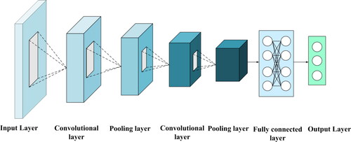
The CNN structure is shown in Figure 1. A complete CNN structure generally includes an input layer, a convolution layer, a pooling layer and an output layer. In the convolutional layer, local features at the same location are extracted by multiple filters instead of sensing the entire feature matrix. Specifically, only the sliding through the filters is required to get all the feature information of the region data. In addition, weight sharing can be realized in the same layer, and these two features can make the network layer deeper and capture more feature information on the premise of ensuring computational efficiency. After the convolution layer, the pooling layer is added to undersample the extracted data features, remove the redundant information in the convolution layer, and further integrate the important data features. Finally, all the extracted feature information is transferred to the full connection layer for feature stitching.

Figure 1. Structure diagram of convolutional neural network.

The convolution operation uses the input data to obtain the feature matrix of the protein data through the convolution operation. The feature of CNN weight sharing makes it use the same set of weight parameters in the whole feature graph of the input data for convolution operation, which enhances some features of the original protein data. In the convolution operation, the eigenvector of the data and the weight parameters in the convolution operation are input for dot product operation, and finally the output matrix with characteristic information is obtained. (1) $$V=\mathit{conv}\left(W,X\right)+b$$(1) (2) $$Y=\mathrm{\varphi }\left(V\right)$$(2)

The operation result of Equation (1)(1) $$V=\mathit{conv}\left(W,X\right)+b$$(1) represents the output of the input data after convolution operation. Where conv represents the convolution operation function, W represents the convolution kernel matrix, X represents the input matrix, b represents the offset. Equation (2)(2) $$Y=\mathrm{\varphi }\left(V\right)$$(2) takes the output of the convolution layer into the active layer as input, and $\varphi (V)$ represents the activation function.

Batch standardization

When designing a network model, the high-dimensional features of protein data can be extracted by increasing the network depth, but it will bring some problems as the network deepens. In the hidden layer, the front and back layers are connected to each other to transfer data features. This connection structure leads to the complexity of parameter updating during training, so when the underlying parameters change slightly, it will lead to low training efficiency and gradient explosion when the underlying parameters are transmitted layer by layer to update this change. To avoid this problem, batch standardization can be added after each convolution layer. After the batch normalization (BN) layer is placed in the ReLU activation layer, it is equivalent to directly normalizing the input of the middle layer of the network, rather than just preprocessing the input layer. Adding a BN layer to neural network training can speed up the training and make the change of energy loss more stable, which avoids excessive jump and finally improves the classification accuracy of the model.

The BN layer processes the protein data of the intermediate layer, such as Equations (3)(3) $${\mu }_{\beta }=\frac{1}{m}\sum _{i=1}^m{x}_i$$(3) and (4)(4) $${\sigma }_{\beta }^2=\frac{1}{m}\sum _{i=1}^m{(x_i-{\mu }_{\beta })}^2$$(4) . First of all, the sample mean and sample variance are calculated for small batches of protein data, and then, as shown in Equation (5)(5) $$\widehat{x_i}\frac{x_i-{\mu }_{\beta }}{\sqrt{{\sigma }_{\beta }^2-\epsilon }}$$(5) , the sample mean and sample variance of small batches of protein data are normalized to the batch of protein data. The purpose of $\mathrm{\epsilon }$ in Equation (5)(5) $$\widehat{x_i}\frac{x_i-{\mu }_{\beta }}{\sqrt{{\sigma }_{\beta }^2-\epsilon }}$$(5) is to avoid the small positive number used when the divisor is 0, and the normalization will limit the expression of the data to the range of 0–1. However, it not only reduces the amount of computation, but also brings new problems, which may restrain the expression ability of the network. In order to avoid this problem, two new parameters are introduced: scale factor Υ and translation factor, they are learned by the Internet itself during training. As shown in Equation (6)(6) $${BN}_{\mathrm{{\rm Y}},\beta }\left(x_i\right)=y_i=\mathrm{{\rm Y}}\widehat{x_i}+\beta$$(6) , x_i is multiplied by Υ to adjust the size of the value, plus $\beta$ to increase the offset to get y_i. After the processing of the BN layer, the training speed is effectively accelerated. Due to the addition of normalization in the middle of the hidden layer, the computational cost is reduced during back propagation, which offers a partial solution to the problem of gradient dispersion in the deep network and improves the generalization ability of the network. (3) $${\mu }_{\beta }=\frac{1}{m}\sum _{i=1}^m{x}_i$$(3) (4) $${\sigma }_{\beta }^2=\frac{1}{m}\sum _{i=1}^m{(x_i-{\mu }_{\beta })}^2$$(4) (5) $$\widehat{x_i}\frac{x_i-{\mu }_{\beta }}{\sqrt{{\sigma }_{\beta }^2-\epsilon }}$$(5) (6) $${BN}_{\mathrm{{\rm Y}},\beta }\left(x_i\right)=y_i=\mathrm{{\rm Y}}\widehat{x_i}+\beta$$(6)

Model

RAdam optimizer

RAdam optimizer is used, which has achieved excellent results in image classification, language modelling, machine translation, etc. Compared with the traditional Adam optimizer, RAdam is more robust to the change of learning rate and can adjust the learning rate dynamically. After multiple experiments, it is proved that the use of RAdam optimizer in the training process can provide better training stability.

In the early stage of training, the optimizer did not get enough protein data, and the adaptive learning rate changed greatly at the beginning of the training. Due to the small amount of data, the choice of learning rate is particularly important. Fortunately, the problem of Adam falling into local optimization can be effectively avoided by using the following approaches. Specifically, when there is less protein data in the early stage of training, we first start the training with a smaller learning rate, and then gradually increase the learning rate to the learning rate used in formal training, and use the learning rate adjustment strategy in formal training in the rest of the training process.

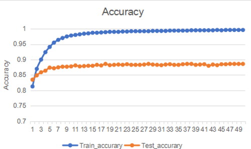
The design idea of RAdam is to use a dynamic heuristic method to provide automatic variance attenuation, which can calculate a preheating heuristic value based on the actual variance encountered, and eliminate the need for manual tuning involved in the training warm-up phase. RAdam establishes a rectifier to dynamically adjust the adaptive momentum, preventing the adaptive momentum from changing so fast that it cannot be expressed as the basic variance function, and uses the rectifier to increase its damping until the variation from the data begins to stabilize. As shown in Figure 2, experiments show that the use of RAdam optimizer can effectively improve the optimization process of the network and improve the accuracy of protein classification.

Figure 2. Training test accuracy rate graph.

ResNet

Compared with the direct mapping of the traditional neural network, the jump connection identity (x) is added to the residual network, and the function of the residual structure is that when the network reaches a certain depth, the neural network has reached the optimal state in the ideal state. If it is further deepened, the network will be degraded, and if the residual network is used, it is only necessary to satisfy the F(x)=0. In practical application, we can fine-tune the model by updating some of the weights of F(x) to achieve the purpose of continuing the high-rate optimization model. (7) $$H\left(x\right)=F\left(x\right)+\mathit{identity}\left(x\right)$$(7)

In Equation (7)(7) $$H\left(x\right)=F\left(x\right)+\mathit{identity}\left(x\right)$$(7) , x represents the input data, F(x) represents the parameter learning algorithm of the main part, identity (x) represents the input data processed by fast connection mapping, identity (x) operation is through quick connection and element-by-element addition operation, and the potential mapping relationship can be better fitted through the cooperation between the residual unit and the main body network.

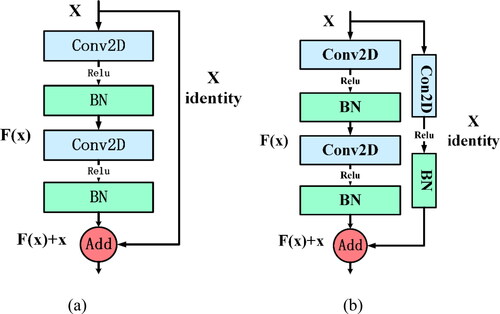
Two kinds of jumping residual structures are designed respectively. The residual structure a is shown in Figure 3(a). In the main body of the residual unit, the BN layer is added to improve the training efficiency, and after each convolution operation, the ReLU activation function is added to increase the nonlinear factors to improve the expression ability of the model. At the same time, the constant quick connection enables the output of one layer to cross several layers directly as the input of the later layer. The residual structure b is shown in Figure 3(b). Convolution network is also used in the main network of residual unit to extract the data features, convolution network and BN operation are also added in the fast connection, and zero-filling operation is added in the convolution layer. This method can not only ensure that the fast connection mapping and function connection match each other in the output dimension, but also fuse the protein data features extracted in the fast connection with the data features extracted from the agent network, so that different data features can be expressed more easily.

Figure 3. Two skipped residual structures. (a) Residual structure a. (b) Residual structure b.

A residual network with 30 convolution layers is designed to extract features from protein data, as shown in network model 4. At the beginning and end of the whole network structure, the shortcut connection is used to simply perform the identity mapping and add its output to the output of the stack layer, which adds neither additional parameters nor computational complexity. The residual structure b is added to the middle module of the whole network structure to better extract data features and increase the differences of different types of protein data.

The structure of ResNet is different from the traditional convolution structure, which makes the forward propagation and gradient back propagation of signals more complex. To stabilize the forward propagation of the signal and the back propagation of the gradient during training, Batch Normalization is added to each convolution neural network in the whole network structure to suppress because the deepening of the network will cause the gradient explosion and gradient disappearance. Then, after each convolution operation, the ReLU activation function is added to map part of the input of the negative interval to zero, which not only improves the sparsity of the network, but also reduces the number of parameters and accelerates the convergence speed of the network. The ReLU activation function has no saturation region, and it also prevents the gradient disappearance caused by the direct mapping of the middle layer of the deep network structure.

After introducing the residual structure, the slight change of the network weight causes a great change in the output. Accordingly, in order to get a good output structure, the weight must be adjusted carefully. Many experiments show that, as shown in Figure 4, the convolution kernel with a convolution window size of 13 to 13 is used to extract features in the first residual module, and the protein data is input into 160 filters for convolution operation. In the second residual module of the residual network, 260 convolution kernels with convolution size of 7 to 7 are used for convolution operation, and smaller convolution windows are used to extract protein features, and the feature information of different locations is fused in the residual unit. Then,270 convolution kernels of size 7 to 7 are used in the third residual module of the network to deeply mine data features. This provides more differential features for the classifier, and a Dense layer is added at the end of the network to integrate the extracted data features. In this way, the differences in the characteristics of different types of protein data are accurately expressed and finally classified by Softmax. The specific model execution parameters are shown in Table 1.

Figure 4. Schematic diagram of Resnet network.

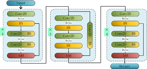
Table 1. Perform parameter settings in the model.

Layer name	Kernel size	Filter size	Output size	Input layer name	Execution round
Input	–	–	20 × 19 × 1	Data
Conv_BN1	13 × 13	160	20 × 19 × 160	Input
BN1	13 × 13	160	20 × 19 × 160	Conv_BN1	4
Conv_BN2	13 × 13	160	20 × 19 × 160	BN1
Conv_BN3	13 × 13	160	20 × 19 × 160	Conv_BN2
Add1	–	–	20 × 19 × 160	BN1 + Conv_BN3
Conv_BN4	7 × 7	260	20 × 19 × 260	Add1
Conv_BN5	7 × 7	260	20 × 19 × 260	Add1	3
Conv_BN6	7 × 7	260	20 × 19 × 260	Conv_BN5
Add2	–	–	20 × 19 × 260	Conv_BN4 + Conv_BN6
Conv_BN7	7 × 7	270	20 × 19 × 270	Add2
Conv_BN8	7 × 7	270	20 × 19 × 270	Add2	4
Conv_BN9	7 × 7	270	20 × 19 × 270	Conv_BN8
Add3	–	–	20 × 19 × 270	Conv_BN7 + Conv_BN9
Dense_1	–	–	64	Add3
Dense_2	–	–	3	Dense_1

Experiment

To quantitatively evaluate the performance of the proposed deep residual network model using different residual units under different conditions, several benchmark data sets were selected for experiments, and six evaluation indexes were used. Furthermore, it is compared with several baseline methods.

Data set and data processing

In the experiment, three common datasets are used: (1) preprocessing datasets from CullPDB [32] in [19]; (2) ASTRAL datasets in [33]; and (3) CASP9, CASP10, CASP11 and CASP12 datasets [34,35]. ASTRAL data sets and CullDB data sets (a total of 15696 proteins after all duplicate proteins have been removed) are filtered based on 25% identity cut, 3 A resolution cut and 0.25 R factor cut. The filtered dataset was merged as the training set, and the CASP9, CASP10, CASP11 and CASP12 datasets were selected as the test set, which contained 122, 99, 81 and 19 protein sequences respectively. Protein data coding follows the settings in reference [24] to ensure the objectivity of the experiment.

At the same time, according to the regulation of DSSP, the secondary structure of a protein is divided into eight categories: H, G, I, E, B, T, S and ‘-’. And these eight classes, according to H,G,I→H; E,B →E; T,S, ‘-’→Other C, are transformed into C (coil), H (helix), E (strand), 3 classes.

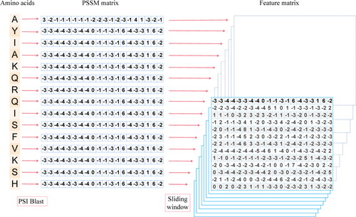
In order to facilitate the data to be sent into the residual network for autonomous learning, a fixed size sliding window is set up in the experiment, centreing on each target amino acid. The amino acid sequence is slid from left to right to extract all the amino acid features in the window. For the window positions at both ends of the protein sequence that are beyond the range of the sequence, the eigenvector is replaced by a zero vector. Figure 5 shows the conversion chart of amino acid sequence data with a window size of 13. The feature model constructed by this method can better express the protein sequence information.

Figure 5. Protein data conversion operation based on sliding window.

Evaluation index

Similar to [18] and [20], three evaluation indicators commonly achieved in previous studies are used to evaluate the accuracy of protein secondary structure prediction. Accuracy rate Q3 measures the percentage of residues that are correctly predicted in the three-class protein secondary structure class, and the expression is as follows: (8) $$\mathrm{Q}3=\frac{N_C+N_E+N_H}{N}\times 100$$(8)

Where N is the total number of amino acid residues, N_C, N_E and N_H respectively represent the correct rate of the secondary structure of the coil, strand and helix. The accuracy of each type of secondary structure can be expressed as (9): (9) $$Q_P=\frac{{TP}_P}{n_p}\times 100$$(9)

Where TP_P is the number of amino acid residues correctly predicted by a certain class, and n_p indicates that the secondary structure is the number of amino acid residues of a certain class. SOV is a measurement method based on secondary structure fragments, which is widely used in CASP competitions. The SOV method measures the secondary structure fragments that are correctly predicted in the prediction of protein secondary structure, rather than evaluating the position of a single residue.

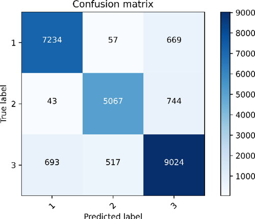
At the same time, the first-level evaluation of confusion matrix is added to use confusion matrix (also known as error matrix, Confusion Matrix) to show the classification effect. As explained [36,37], the confusion matrix is mainly calculated based on four parameters: the real value is positive and the protein classification model considers the number of positive (True Positive = TP). The real value is positive, and the protein classification model thinks that it is the number of negative (False Negative = FN). The real value is negative, and the protein classification model thinks that it is the number of positive (False Positive = FP). The real value is negative, and the protein classification model thinks that it is the number of negative (True Negative = TN). The four indicators are presented together in the table, showing the confusion matrix, which is shown in Figure 6.

Figure 6. Confusion matrix diagram.

Comparative experiment

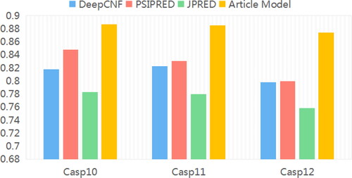
In order to further verify its classification performance, this model is compared with several mainstream methods, including DeepCNF, PSRSM, PSIPRED, JPRED, etc. According to Table 2, in the three test sets of CASP10, CASP11 and CASP12, the prediction results of the proposed model are improved compared to DeepCNF, PSIPRED, JPRED and DeepNRN models. In addition, on the CASP10 data set, the accuracy of this model for protein structure prediction is significantly improved, and the result is up to 0.887. Compared with the JPRED model, the classification accuracy is improved by more than 10%, and compared with the other two models, the classification accuracy is also improved by more than 4%, indicating that the model can effectively extract protein data features, increase the differences between categories, and thus, improve the accuracy of classification.

Table 2. Comparison of prediction accuracy of each model on 4 datasets.

Methods	CASP10	CASP11	CASP12	CASP9
DeepCNF [18]	0.818	0.823	0.798	–
PSIPRED [9]	0.848	0.831	0.800	–
JPRED [23]	0.783	0.780	0.759	–
DeepNRN [6]	0.856	0.856	0.834	–
This paper	0.887	0.885	0.874	0.883

This model is fully validated on the three data sets of CASP10, CASP11 and CASP12, as shown in the bar chart of Figure 7. The results show that it can improve the classification effect of different types of protein data in three data sets. Compared with other models, this model can obtain the local and global characteristic information of protein structure more comprehensively, because it uses two kinds of convolution kernels of different numbers and sizes to obtain the characteristic information of protein structure. On the whole, the prediction accuracy of this model is significantly higher than that of other comparative models, indicating that it fully extracts the type information coding and biological evolutionary structure information of amino acids, and effectively interacts with the extracted local and long-range feature information, which effectively improves the prediction accuracy of the secondary structure of three-classification proteins.

Figure 7. Model comparison histogram.

Conclusions

In this work, a deep residual network with different residual units is designed. Specifically, it can effectively extract the local and global features of protein data through two different residual units, and at the same time deepen the depth of the network. It can be proposed to a deeper level of abstract data features, thereby providing a more comprehensive difference data information for the classifier, and improving the classification accuracy of the model. In addition, the RAdam optimizer is used to optimize the training process, and its dynamic heuristic method is used to provide automated variance attenuation, which effectively improves the classification accuracy of protein data while ensuring the stability in the initial training stage. Ultimately, multiple experimental data sets confirmed that this method has better classification performance. In the next work, we will continue to optimize on the basis of the model, and consider introducing a confrontation network to improve the model’s ability to generalize data.

Author contributions

Cheng and Zhao Carried out all the experiments, and collected all data. Zhao provided the concept. Xu wrote the manuscript. All authors polished the manuscript.

Disclosure statement

All the authors declare that there are no conflicts of interests regarding the publication of this article.

Data availability statement

The data used to support the findings of this study are available from the corresponding author upon request.

The raw data used in our manuscript are all publicly available public datasets and can be found at the following URL:

https://doi.org/10.1093/nar/gkt1240

https://predictioncenter.org/download_area/CASP9/targets/

https://predictioncenter.org/download_area/CASP10/targets/

https://predictioncenter.org/download_area/CASP11/targets/

https://predictioncenter.org/download_area/CASP12/targets/

This experiment has performed data processing on the original data set, and it is currently impossible to disclose the processed data because these data are also part of the ongoing research. After accepting this article, the data used to support the findings of this study are available from the corresponding author upon request.

Additional information

Funding

This work is supported by Key Research and Development Project of Shandong Province (2019JZZY020124), China, and Natural Science Foundation of Shandong Province (ZR2017MF056), China.

References

- Alexey D, Christian C, James P, et al. Jpred4: a protein secondary structure prediction server. Nucleic Acids Res. 2015;43(W1):W389–W394.
- Schlessinger A, Rost B. Protein flexibility and rigidity predicted from sequence. Proteins-Struct Funct Bioinform. 2005;61(1):115–126.
- Radivojac P, Iakoucheva LM, Oldfield CJ, et al. Intrinsic disorder and functional proteomics. Biophys J. 2007;92(5):1439–1456.
- Abdennaji I, Zaied M, Girault JM. Prediction of protein structural class based on symmetrical recurrence quantification analysis. Comput Biol Chem. 2021;92:107450.
- Torrisi M, Pollastri G, Le Q. Deep learning methods in protein structure prediction. Comput Struct Biotechnol J. 2020; 18:1301–1310.
- Fang C, Shang Y, Xu D. A new deep neighbor residual network for protein secondary structure prediction. 2017 IEEE 29th International Conference on Tools with Artificial Intelligence (ICTAI), Boston, MA, USA; 2017. p. 66–71.
- Santoni D. The impact of codon choice on translation process in saccharomyces cerevisiae: folding class, protein function and secondary structure. J Theor Biol. 2021;526:110806.
- Rost B, Sander C. Improved prediction of protein secondary structure by use of sequence profiles and neural networks. Proc Natl Acad Sci U S A. 1993;90(16):7558–7562.
- Jones DT. Protein secondary structure prediction based on position-specific scoring matrices. J Mol Biol. 1999;292(2):195–202.
- Taherzadeh G, Zhou Y, Liew AW, et al. Sequence-based prediction of protein-carbohydrate binding sites using support vector machines. J Chem Inf Model. 2016;56(10):2115–2122.
- Dor O, Zhou Y. Achieving 80% ten-fold cross-validated accuracy for secondary structure prediction by large-scale training. Proteins Struct Funct Bioinform. 2007;66(4):838–845.
- Chou KC. Prediction of protein cellular attributes using pseudo-amino acid composition. Proteins Struct Funct Bioinform. 2001;43(3):246–255.
- Gao CF, Wu XY. Feature extraction method for proteins based on markov tripeptide by compressive sensing. BMC Bioinform. 2018;19(1):229–232.
- Kurniawan I, Haryanto T, Hasibuan LS, et al. Combining pssm and physicochemical feature for protein structure prediction with support vector machine. J Phys: Conf Ser. 2017;835:012006.
- Guermeur Y, Pollastri G, Elisseeff A, et al. Combining protein secondary structure prediction models with ensemble methods of optimal complexity. Neurocomputing. 2004;56:305–327.
- Pakhrin SC, Shrestha B, Adhikari B, et al. Deep learning-based advances in protein structure prediction. IJMS. 2021;22(11):5553.
- Fang C, Shang Y, Xu D. MUFOLD-SS: new deep inception-inside-inception networks for protein secondary structure prediction. Proteins. 2018;86(5):592–598.
- Wang S, Peng J, Ma J, et al. Protein secondary structure prediction using deep convolutional neural fields. Sci Rep. 2016;6:18962.
- Zhen L, Yu Y. Protein secondary structure prediction using cascaded convolutional and recurrent neural networks. In: International Joint Conference on Artificial Intelligence (IJCAI); New York City; July 9, 2016.
- Busia A, Jaitly N. Next-step conditioned deep convolutional neural networks improve protein secondary structure prediction. In: Conference on Intelligent Systems for MolecularBiology and European Conference on Computational Biology (ISMB/ECCB 2017); Leesburg: International Society of Computational Biology; 2017.
- Rhys H, Yang Y, Kuldip P, et al. Capturing non-local interactions by long short term memory bidirectional recurrent neural networks for improving prediction of protein secondary structure, backbone angles, contact numbers, and solvent accessibility. Bioinformatics. 2017;18:18.
- Heffernan R, Paliwal K, Lyons J, et al. Improving prediction of secondary structure, local backbone angles, and solvent accessible surface area of proteins by iterative deep learning. Sci Rep. 2015;5:11476.
- Christian C, Barber JD, Barton GJ. The jpred 3 secondary structure prediction server. Nucleic Acids Res. 2008;36(Web Server issue):W197–W201.
- Ma Y, Liu Y, Cheng J. Protein secondary structure prediction based on data partition and semi-random subspace method. Sci Rep. 2018;8(1):9856.
- He K, Zhang X, Ren S, et al. Identity mappings in deep residual networks. In: B. Leibe et al. (Eds.), Computer vision – ECCV 2016. ECCV 2016, Part IV, LNCS 9908. Lecture notes in computer science, vol. 9908, pp. 630–645. Cham: Springer; 2016.
- Zhang K, Sun M, Han TX, et al. Residual networks of residual networks: multilevel residual networks. IEEE Trans Circuits Syst Video Technol. 2018;28(6):1303–1314. http://dx.doi.org/10.1109/TCSVT.2017.2654543.
- Huang G, Liu Z, Laurens V, et al. Densely connected convolutional networks. 2017 IEEE Conference on Computer Vision and Pattern Recognition (CVPR), Honolulu, HI, USA; 2017. p. 2261–2269.
- Szegedy C, Vanhoucke V, Ioffe S, et al. Rethinking the inception architecture for computer vision. In: 2016 IEEE Conference on Computer Vision and Pattern Recognition (CVPR); Las Vegas; 2016. p. 2818–2826.
- Ioffe S, Szegedy C. Batch normalization: accelerating deep network training by reducing internal covariate shift. In: Proceedings of the 32nd International Conference on Machine Learning, Lille, France; 2015. p. 448–456.
- Srivastava N, Hinton G, Krizhevsky A, et al. Dropout: a simple way to prevent neural networks from overfitting. J Mach Learn Res. 2014;15:1929–1958.
- Gongora-Canul C, Fernandez-Campos M. Wheat spike blast image classification using deep convolutional neural networks. Front Plant Sci. 2021;12:673505.
- Wang G, Dunbrack RL. Pisces: a protein sequence culling server. Bioinformatics. 2003;19(12):1589–1591.
- Fox NK, Brenner SE, John-Marc C. Scope: structural classification of proteins-extended, integrating SCOP and ASTRAL data and classification of new structures. Nucleic Acids Res. 2014;42(Database issue):D304–D309.
- Moult J, Fidelis K, Zemla A, et al. Critical assessment of methods of protein structure prediction (CASP)-round v. Proteins Struct Funct Bioinform. 2003;53 Suppl 6:334–339. DOI:10.1002/prot.10556.
- Moult J, Fidelis K, Kryshtafovych A, et al. Critical assessment of methods of protein structure prediction (CASP)-round ix. Proteins Struct Funct Bioinform. 2011;79 Suppl 10(010):1–5.
- Moult J, Fidelis K, Kryshtafovych A, et al. Critical assessment of methods of protein structure prediction (CASP) - round x. Proteins. 2014;82:1–9.
- Zhang W, Liu C. Research on human abnormal behavior detection based on deep learning. In: 2020 International Conference on Virtual Reality and Intelligent Systems (ICVRIS), Zhangjiajie, Hunan, China; 2020. p. 973–978.