Modeling and structural control of a building with holonomic constraints

ABSTRACT

In this study, we propose to evaluate structural control systems in terms of mechanical impedance and the peak of energy stored by the structure. Our main hypothesis is that the higher the mechanical impedance, the lower the peak of energy reached by the structure. This peak is calculated as the maximum of the difference between the energy injected by the seism and the energy dissipated as heat by viscous dampers. To support our claim, we performed numerical simulations on a three-story planar building comprising 12 revolute and four prismatic joints. Instead of using a linear mass-spring-damper model, we simulated a set of nonlinear equations given by the Newton-Euler (NE) algorithm, which has been widely used in robotics, but rarely in structural control. For energy dissipation, we compared a proportional derivative (PD) with a computed torque control (CTC). Simulation results for the CTC indicate that when all parameters of the structure are perfectly known, the deviations of the revolute and prismatic joints with respect to their nominal values are close to zero. This feature leads to almost null energy dissipation, but also reduces the energy transferred by the seism to the structure.

KEYWORDS:

• Structural control
• dynamic model
• simulation
• holonomic constraints

1. Introduction

Structures must be supervised to ensure their resistance to seismic threats and to avoid risks to human beings (Güemes et al. 2020). To avoid the collapse of a structure during earthquakes, the structure must dissipate seismic energy (Zhang et al. 2020). To increase safety, energy dissipation techniques have been used to modify structural dynamics (Oviedo and Duque 2006). The most used actuators to dissipate energy in buildings are viscous dampers. They are based on the use of active, passive, or semi-active elements, whose performance depends on both the excitation applied to the structure and the amount of energy to be dissipated. These techniques are based on a combination of stiffness and energy dissipation capacity in the inelastic range of the structure (Swartz 2011). The design, model and control of dampers for mitigating the energy of earthquakes have been studied for many authors. Yang et al. (2020) model and control a shear-mode rotational damper for mitigating vibrations in buildings. Yang et al. (Yang et al. 2016) control a magnetorheological elastomer base isolation system using a second order sliding approach. Gu et al. (2017) propose a smart base for vibration isolation that utilises a semi-active magnetorheological elastomer controlled by learning-based inverse model. The latter (Gu et al. 2019) presented an optimal neuro-fuzzy controller for the same system.

Structural control is an active area of research (Chiaia et al. 2020; Shih and Sung 2020; Reksowardojo and Senatore 2020; Di Girolamo et al. 2020). (Zhang and Ou 2015) propose an electromagnetic mass driver system (EMDS) for the control of structural vibrations. The EMDS consists of a rod made of tiny permanent magnets, which moves horizontally along the axis of an electric coil fixed to the structure to be controlled. The Lorenz force exerted on the coil counteracts earthquake-induced vibrations and varies with the voltage applied to the coil. This means that there is no mechanical contact between the rod and the structure, which leads to an unlimited mass stroke, lower operating noise, and limited wearing of moving parts. In addition, EMDS is faster and simpler than active mass dampers based on hydraulic systems or electric motors.

Despite the high success of active mass dampers for vibration control of civil structures; they have proven to be ineffective in controlling the swing vibrations of suspended structures such as bridges, pipelines, and wind turbines. This problem has motivated (Zhang, Li, and Ou 2009) to propose inertial dampers, which, unlike active mass dampers, produce rotary instead of linear motion. In Zhang and Wang (2020), the authors present a rotary inertia damper, whose torque is calculated by a linear quadratic regulator. The numerical and experimental results, obtained on a vertical bar fixed to a shaking table, show the effectiveness of the technique to mitigate swing vibrations.

The dynamic modelling is a fundamental aspect for the design of controllers that dissipate the energy produced by an earthquake and avoid the collapse of the structure (Munteanu et al. 2020). Many works in the literature present mathematical models of structures (Pieczonka et al. 2013; Astroza and Alessandri 2019; Bouayed, Hamdi, and Rachik 2013). The design of structural controllers requires dynamic modelling (Cramer et al. 2016; Cao, Ouyang, and Cheng 2019; Renzi and Serino 2004; Ziyaeifar, Gidfar, and Nekooei 2012) and identification of structural parameters (Zhao et al. 2020; Yan, Sun, and Buyukozturk 2017; Soliman, Tait, and El Damatty 2017). An example of model-based control is presented in (Zhang 2014), where the authors compare four control strategies for suppressing wind-induced vibrations in a 76-story building. The first and second strategies are structural interleaved control and structural adjacent reaction wall (STA), respectively, using one actuator per floor. The other two strategies are the active mass damper and the semi-active mass damper (SAMD), which employ a single actuator, commonly located on top of the building. The main conclusion of (Zhang 2014) is that SAMD achieves similar performance that STA but at lower cost.

In this article, a three-story building is modelled as a closed kinematic chain with holonomic constraints. Unlike the simplified models presented in (Li et al. 2017), (Mohamed and Lakhdar 2016) and (Makisha 2019), the mathematical model proposed here represents the complete dynamics of the structure under study and allows comparison of different model-based control strategies (Bravo et al. 2019). The main contribution of this work is to study structural control systems in terms of the mechanical impedance and the energy stored by a structure. Here, we compare through simulation the performance of PD and CTC controllers for a mechanical three-story structure comprising 12 revolute and four prismatic joints (Fabien 2008).

2. Theoretical background

In this section, we explain the concept of mechanical impedance (Yang and Soh 2009) and its relation with the maximal kinetic energy stored by a structure when excited by an external force, such as wind or an earthquake.

The mechanical impedance quantifies the force exerted by a system in opposition to changes in its velocity. Mathematically, the mechanical impedance is defined as the quotient between a change in the input force and the corresponding change in velocity (Khalil and Dombre 2004). The stiffer a system is, the higher its mechanical impedance. In linear systems, the mechanical impedance is defined as the Laplace transform of the force divided by the Laplace transform of the velocity (Richardson et al. 2005).

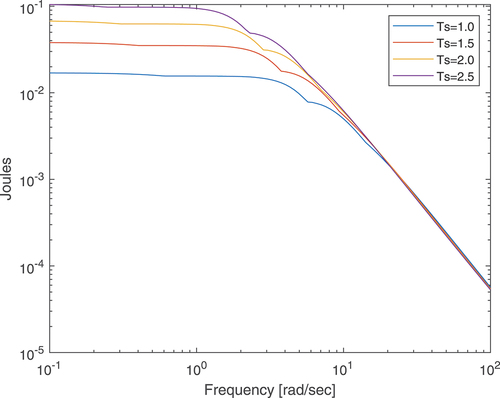
The settling time of a structure influences its mechanical impedance. For example, the settling time of a mass-spring-damper system is $T_s$ when the spring constant is $k=16m/({\xi }^2{T}_s^2)$, the damper constant is $\beta =8m/T_s$, and the mass is $m$. This means that low values of $T_s$ (fast structural response) implies high values of $k$ and $b$. The maximum energy transferred to a structure in a given time interval depends on both the magnitude and the phase of its mechanical impedance. For constant phase, the lower the magnitude, the higher the maximum input energy, and for constant magnitude, the closer to zero the phase, the higher the maximum input energy. This last statement is explained by the maximum power transfer theorem (Nambiar 1969). Figure 1 shows the maximum input energy transferred to a linear mass-spring-damper system as a function of frequency. From this figure, it can be seen that at low frequency, the lower $T_s$, the lower the maximum input energy, and for high frequencies this relation is the opposite. This behaviour is explained by Table 1, which shows that at low frequencies the phase is almost constant and the magnitude decreases when $T_s$ increases. At high frequencies, the magnitude is almost constant and the phase is nearest to zero as $T_s$ increases.

Table 1. Impedance of a mass-spring-damper system for low and high frequencies, when $\xi =0.707$ and $m=1$.

	$\omega =0.1$ rad/s		$\omega =10$ rad/s
$T_s$	$|z|$	$\mathrm{\angle }z$	$|z|$	$\mathrm{\angle }z$
$1.0$	$320.10$	$-{88.57}^o$	$10.50$	${40.36}^o$
$1.5$	$142.27$	$-{87.85}^o$	$10.10$	${58.13}^o$
$2.0$	$80.02$	$-{87.13}^o$	$10.03$	${66.50}^o$
$2.5$	$51.22$	$-{86.42}^o$	$10.01$	${71.36}^o$

Figure 1 was obtained by solving the following maximisation problem for different frequencies:

$E_{max}=\underset{t\ge 0}{max}{\int }_0^{t}f(\lambda )v(\lambda )-\beta v(\lambda {)}^{2}d\lambda$

When $f(t)=cos(\omega t)$ is the input force and $v(t)$ the velocity of the mass, the product $f(t)v(t)$ is the mechanical input power and $\beta v(t{)}^2$ is the power dissipated by the damper as heat.

Figure 2 shows that the lower $T_s$, the lower the maximum of the energy stored by the structure.

Figure 1. Maximal input energy transferred to a mass-spring-damper system when $\xi =0.707$ and $m=1$.

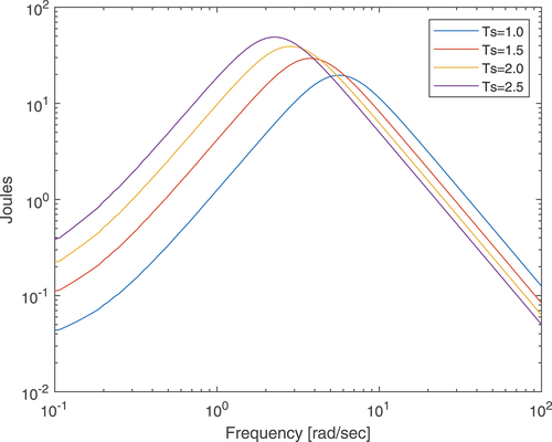
Figure 2. Maximal stored energy by a mass-spring-damper system.

3. Structure modelling

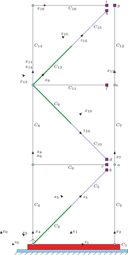
Although the planar building presented in Figure 3 has 12 revolute and 4 prismatic joints, it only has 4 degrees of freedom. The actuator $P_1$ represents the seismic forces acting on the base of the building, while $P_5$, $P_{10}$ and $P_{15}$ are responsible for energy dissipation. The length of the walls and floors of the structure are $4.85$ and $4.00[m]$ respectively. The $P_5$, $P_{10}$ and $P_{15}$ actuators must keep the crossbar length at $L^d=\sqrt{{4.85}^2+{4.00}^2}[m]$, in order to guarantee right angles between walls and floors.

Figure 3. Structure mobility analysis.

3.1. Geometric model of the structure

The definition of the reference axes for Figure 3 begins with the construction of a tree structure derived from the original system. By tree, we mean a structure with no closed loop kinematic chains (Khalil and Dombre 2004). The tree structure is obtained by separating the points $a$, $b$, $\dots$, $i$ of Figure 4, which correspond to passive joints (Cheng and Tian 1992).

Figure 4. Tree equivalent structure obtained from 3.

Once the reference axes for each body have been established, the table of kinematic parameters is generated. The table comprises six geometric parameters (Khalil and Dombre 2004) $({\gamma }_j,b_j,{\alpha }_j,d_j,{\theta }_j,r_j)$ that relate all the linear and angular dimensions of the building:

The kinematic parameters of Table 2 define the matrix (1), which transforms Cartesian positions from the reference frame $j$ to the reference frame $a_j$. This last frame indicates the body that precedes the body $j$. For example, Figure 4 and Table 2 show that the body $8$ is the common predecessor of the bodies $9$, $11$, $13$, and $14$. In this manner $a_9=a_{11}=a_{13}=a_{14}=8$.

(1) ${ }^{a(j)}{T}_j=\left[\begin{array}{cccc}C{\gamma }_{j}C{\theta }_j-S{\gamma }_{j}C{\alpha }_{j}S{\theta }_j& -C{\gamma }_{j}S{\theta }_j-S{\gamma }_{j}C{\alpha }_{j}C{\theta }_j& S{\gamma }_{j}S{\alpha }_j& d_{j}C{\gamma }_j+r_{j}S{\gamma }_{j}S{\alpha }_j\\ S{\gamma }_{j}C{\theta }_j+C{\gamma }_{j}C{\alpha }_{j}S{\theta }_j& -S{\gamma }_{j}S{\theta }_j+C{\gamma }_{j}C{\alpha }_{j}C{\theta }_j& -C{\gamma }_{j}S{\alpha }_j& d_{j}S{\gamma }_j-r_{j}C{\gamma }_{j}S{\alpha }_j\\ S{\alpha }_{j}S{\theta }_j& S{\alpha }_{j}C{\theta }_j& C{\alpha }_j& r_{j}C{\alpha }_j+b_j\\ 0& 0& 0& 1\end{array}\right]$(1)

Table 2. Geometric parameters (Figure 4).

$j$	$a_j$	${\sigma }_j$	${\gamma }_j$	$b_j$	${\alpha }_j$	$d_j$	${\theta }_j$	$r_j$
$1$	$0$	$1$	$0$	$0$	$0$	$0$	$0$	$q_1$
$2$	$1$	$0$	$0$	$+B2$	$-\pi /2$	$0$	$q_2$	$0$
$3$	$1$	$0$	$0$	$-B2$	$-\pi /2$	$0$	$q_3$	$0$
$4$	$1$	$0$	$0$	$-B2$	$-\pi /2$	$0$	$q_4$	$0$
$5$	$3$	$1$	$0$	$0$	$+\pi /2$	$0$	$0$	$q_5$
$6$	$4$	$0$	$0$	$0$	$0$	$D_6$	$q_6$	$0$
$7$	$2$	$0$	$0$	$0$	$0$	$D_7$	$q_7$	$0$
$8$	$4$	$0$	$0$	$0$	$0$	$D_8$	$q_8$	$0$
$9$	$8$	$0$	$0$	$0$	$0$	$D_9$	$q_9$	$0$
$10$	$9$	$1$	$0$	$0$	$+\pi /2$	$0$	$0$	$q_{10}$
$11$	$8$	$0$	$0$	$0$	$0$	$D_{11}$	$q_{11}$	$0$
$12$	$7$	$0$	$0$	$0$	$0$	$D_{12}$	$q_{12}$	$0$
$13$	$8$	$0$	$0$	$0$	$0$	$D_{13}$	$q_{13}$	$0$
$14$	$8$	$0$	$0$	$0$	$0$	$D_{14}$	$q_{14}$	$0$
$15$	$13$	$1$	$0$	$0$	$+\pi /2$	$0$	$0$	$q_{15}$
$16$	$14$	$0$	$0$	$0$	$0$	$D_{16}$	$q_{16}$	$0$

In Equation (1)(1) ${ }^{a(j)}{T}_j=\left[\begin{array}{cccc}C{\gamma }_{j}C{\theta }_j-S{\gamma }_{j}C{\alpha }_{j}S{\theta }_j& -C{\gamma }_{j}S{\theta }_j-S{\gamma }_{j}C{\alpha }_{j}C{\theta }_j& S{\gamma }_{j}S{\alpha }_j& d_{j}C{\gamma }_j+r_{j}S{\gamma }_{j}S{\alpha }_j\\ S{\gamma }_{j}C{\theta }_j+C{\gamma }_{j}C{\alpha }_{j}S{\theta }_j& -S{\gamma }_{j}S{\theta }_j+C{\gamma }_{j}C{\alpha }_{j}C{\theta }_j& -C{\gamma }_{j}S{\alpha }_j& d_{j}S{\gamma }_j-r_{j}C{\gamma }_{j}S{\alpha }_j\\ S{\alpha }_{j}S{\theta }_j& S{\alpha }_{j}C{\theta }_j& C{\alpha }_j& r_{j}C{\alpha }_j+b_j\\ 0& 0& 0& 1\end{array}\right]$(1) , the symbols $C$ and $S$ denote the cosine and sine functions, respectively. For example, $S{\gamma }_{j}C{\theta }_j$ represents $sin\left({\gamma }_j\right)cos\left({\theta }_j\right)$.

3.2. Holonomic constraints

To transform the tree structure of Figure 4 in the closed kinematic chain of Figure 3, the Cartesian positions of points $a$, $b$, $c$ y $d$ must coincide during simulation. For the second level, the equality constraint must hold for points $f$ and $e$, and for the third level, between $g$, $h$ and $i$. In this manner, the aforementioned points must satisfy

(2) $\left[\begin{array}{c}{ }^0{p}_{\mathrm{a}}{-}^0{p}_{\mathrm{b}}\\ { }^0{p}_{\mathrm{a}}{-}^0{p}_{\mathrm{c}}\\ { }^0{p}_{\mathrm{a}}{-}^0{p}_{\mathrm{d}}\\ { }^0{p}_{\mathrm{e}}{-}^0{p}_{\mathrm{f}}\\ { }^0{p}_{\mathrm{g}}{-}^0{p}_{\mathrm{h}}\\ { }^0{p}_{\mathrm{g}}{-}^0{p}_{\mathrm{i}}\end{array}\right]=0$(2)

Where ${ }^0{p}_{\mathrm{a}}\in I{R}^2$, $\dots$, ${ }^0{p}_{\mathrm{i}}\in I{R}^2$ are Cartesian positions of points $a$ to $i$ with respect to reference system $⟨x_0,y_0⟩$. If (2) is derived with respect to time, then the velocity constraint is obtained

(3) $\left[\begin{array}{c}{ }^0{v}_{\mathrm{a}}{-}^0{v}_{\mathrm{b}}\\ { }^0{v}_{\mathrm{a}}{-}^0{v}_{\mathrm{c}}\\ { }^0{v}_{\mathrm{a}}{-}^0{v}_{\mathrm{d}}\\ { }^0{v}_{\mathrm{e}}{-}^0{v}_{\mathrm{f}}\\ { }^0{v}_{\mathrm{g}}{-}^0{v}_{\mathrm{h}}\\ { }^0{v}_{\mathrm{g}}{-}^0{v}_{\mathrm{i}}\end{array}\right]=\underset{J(q)}{\underbrace{\left[\begin{array}{c}{J}_a(q)-J_b(q)\\ J_a(q)-J_c(q)\\ J_a(q)-J_d(q)\\ J_e(q)-J_f(q)\\ J_g(q)-J_h(q)\\ J_g(q)-J_i(q)\end{array}\right]}}\dot{q}=0$(3)

$J_a(q)\in I{R}^{2\times 16}$ relates $\dot{q}\in I{R}^{16}$ with the velocity of the point $a$ of the structure (Figure 4). The velocity ${ }^0{v}_{\mathrm{a}}$ is measured with respect to the immobile frame $⟨x_0,y_0⟩$. Thereby, ${ }^0{v}_{\mathrm{a}}=J_a(q)\dot{q}$. Matrix $J_b(q)\in I{R}^{2\times 16}$, $J_c(q)\in I{R}^{2\times 16}$, $J_d(q)\in I{R}^{2\times 16}$, $J_e(q)\in I{R}^{2\times 16}$, $J_f(q)\in I{R}^{2\times 16}$, $J_g(q)\in I{R}^{2\times 16}$, $J_h(q)\in I{R}^{2\times 16}$ and $J_i(q)\in I{R}^{2\times 16}$ are used to calculate the velocities of the points $b$, $c$, $d$, $e$, $f$, $g$, $h$ e $i$ with respect to the frame $⟨x_0,y_0⟩$, respectively. Constraint Equation (3)(3) $\left[\begin{array}{c}{ }^0{v}_{\mathrm{a}}{-}^0{v}_{\mathrm{b}}\\ { }^0{v}_{\mathrm{a}}{-}^0{v}_{\mathrm{c}}\\ { }^0{v}_{\mathrm{a}}{-}^0{v}_{\mathrm{d}}\\ { }^0{v}_{\mathrm{e}}{-}^0{v}_{\mathrm{f}}\\ { }^0{v}_{\mathrm{g}}{-}^0{v}_{\mathrm{h}}\\ { }^0{v}_{\mathrm{g}}{-}^0{v}_{\mathrm{i}}\end{array}\right]=\underset{J(q)}{\underbrace{\left[\begin{array}{c}{J}_a(q)-J_b(q)\\ J_a(q)-J_c(q)\\ J_a(q)-J_d(q)\\ J_e(q)-J_f(q)\\ J_g(q)-J_h(q)\\ J_g(q)-J_i(q)\end{array}\right]}}\dot{q}=0$(3) should be derived with respect to time to involve the acceleration vector $\ddot{q}$.

(4) $\begin{array}{cc}\left[\begin{array}{c}{ }^{\mathrm{g}}{\dot{v}}_{\mathrm{a}}{-}^{\mathrm{g}}{\dot{v}}_{\mathrm{b}}\\ { }^{\mathrm{g}}{\dot{v}}_{\mathrm{a}}{-}^{\mathrm{g}}{\dot{v}}_{\mathrm{c}}\\ { }^{\mathrm{g}}{\dot{v}}_{\mathrm{a}}{-}^{\mathrm{g}}{\dot{v}}_{\mathrm{d}}\\ { }^{\mathrm{g}}{\dot{v}}_{\mathrm{e}}{-}^{\mathrm{g}}{\dot{v}}_{\mathrm{f}}\\ { }^{\mathrm{g}}{\dot{v}}_{\mathrm{g}}{-}^{\mathrm{g}}{\dot{v}}_{\mathrm{h}}\\ { }^{\mathrm{g}}{\dot{v}}_{\mathrm{g}}{-}^{\mathrm{g}}{\dot{v}}_{\mathrm{i}}\end{array}\right]& =\underset{\mathbf{J}(q)}{\underbrace{\left[\begin{array}{c}{J}_a(q)-J_b(q)\\ J_a(q)-J_c(q)\\ J_a(q)-J_d(q)\\ J_e(q)-J_f(q)\\ J_g(q)-J_h(q)\\ J_g(q)-J_i(q)\end{array}\right]}}\ddot{q}+\underset{R(q,\dot{q})}{\underbrace{\left[\begin{array}{c}{R}_a(q,\dot{q})-R_b(q,\dot{q})\\ R_a(q,\dot{q})-R_c(q,\dot{q})\\ R_a(q,\dot{q})-R_d(q,\dot{q})\\ R_e(q,\dot{q})-R_f(q,\dot{q})\\ R_g(q,\dot{q})-R_h(q,\dot{q})\\ R_g(q,\dot{q})-R_i(q,\dot{q})\end{array}\right]}}\\ \hspace{0.17em}& =0\\ \hspace{0.17em}& \hspace{0.17em}\end{array}$(4)

Thus, accelerations must satisfy the following constraint:

(5) $\mathbf{J}(q)\ddot{q}+R(q,\dot{q})=0$(5)

3.3. Dynamic model of the structure

Closed kinematic chains are modelled using the following principle:

Tree mechanism + Holonomic constraints = Closed kinematic chain

The above equality implies that if a vector of forces $F$ is added to the direct dynamic model of the tree structure and this vector ensures compliance of the holonomic constraints, then the resulting structure will be a closed kinematic chain (Fabien 2008):

(6) $\mathbf{A}(q)\ddot{q}+H(q,\dot{q})=\mathbf{B}\mathrm{\Gamma }+{\mathbf{J}}^{\mathrm{T}}(q)F$(6)

Being $q\in I{R}^{16}$, $\dot{q}\in I{R}^{16}$ and $\ddot{q}\in I{R}^{16}$, vectors of positions, velocities and generalised accelerations, respectively. $\mathbf{A}\left(q\right)\in I{R}^{16\times 16}$ is the inertia matrix $H\left(q,\dot{q}\right)\in I{R}^{16}$ the vector of centrifugal, gravitational, and Coriolis forces. $F\in I{R}^{12}$ contains the forces that ensure compliance of holonomic constraints, $\mathrm{\Gamma }\in I{R}^4$ is the vector with the forces exerted by the actuators $P_1$, $P_5$, $P_{10}$ and $P_{15}$. Matrix $\mathbf{B}\in I{R}^{16\times 4}$, contains ones and zeros, and satisfies the following property:

(7) $\mathbf{B}\mathrm{\Gamma }=\left[\begin{array}{c}{\mathrm{\Gamma }}_1\\ {\mathbf{0}}_{3\times 1}\\ {\mathrm{\Gamma }}_5\\ {\mathbf{0}}_{4\times 1}\\ {\mathrm{\Gamma }}_{10}\\ {\mathbf{0}}_{4\times 1}\\ {\mathrm{\Gamma }}_{15}\\ 0\end{array}\right]$(7)

${\mathbf{0}}_{3\times 1}$ y ${\mathbf{0}}_{4\times 1}$ are column vectors with three and four zeros, respectively. The product $\mathbf{B}\mathrm{\Gamma }$ indicates that only coordinates $q_1,q_5,q_{10},q_{15}$ are actuated. To find $\ddot{q}$ and $F$ at each time, the following equation must be solved:

(8) $\left[\begin{array}{cc}\mathbf{A}& -{\mathbf{J}}^{\mathrm{T}}\\ \mathbf{J}& 0\end{array}\right]\left[\begin{array}{c}\ddot{q}\\ F\end{array}\right]=\left[\begin{array}{c}\mathrm{\Gamma }-H(q,\dot{q})\\ -R(q,\dot{q})\end{array}\right]$(8)

Vector $F$ ensures that acceleration constraints are met (Equation (5)(5) $\mathbf{J}(q)\ddot{q}+R(q,\dot{q})=0$(5) ). However, to satisfy the velocity and position constraints, it is necessary that the initial conditions $q(0)$ and $\dot{q}(0)$ satisfy Equations (2)(2) $\left[\begin{array}{c}{ }^0{p}_{\mathrm{a}}{-}^0{p}_{\mathrm{b}}\\ { }^0{p}_{\mathrm{a}}{-}^0{p}_{\mathrm{c}}\\ { }^0{p}_{\mathrm{a}}{-}^0{p}_{\mathrm{d}}\\ { }^0{p}_{\mathrm{e}}{-}^0{p}_{\mathrm{f}}\\ { }^0{p}_{\mathrm{g}}{-}^0{p}_{\mathrm{h}}\\ { }^0{p}_{\mathrm{g}}{-}^0{p}_{\mathrm{i}}\end{array}\right]=0$(2) and (3(3) $\left[\begin{array}{c}{ }^0{v}_{\mathrm{a}}{-}^0{v}_{\mathrm{b}}\\ { }^0{v}_{\mathrm{a}}{-}^0{v}_{\mathrm{c}}\\ { }^0{v}_{\mathrm{a}}{-}^0{v}_{\mathrm{d}}\\ { }^0{v}_{\mathrm{e}}{-}^0{v}_{\mathrm{f}}\\ { }^0{v}_{\mathrm{g}}{-}^0{v}_{\mathrm{h}}\\ { }^0{v}_{\mathrm{g}}{-}^0{v}_{\mathrm{i}}\end{array}\right]=\underset{J(q)}{\underbrace{\left[\begin{array}{c}{J}_a(q)-J_b(q)\\ J_a(q)-J_c(q)\\ J_a(q)-J_d(q)\\ J_e(q)-J_f(q)\\ J_g(q)-J_h(q)\\ J_g(q)-J_i(q)\end{array}\right]}}\dot{q}=0$(3) ).

4. Structural control

Civil structures employ automatic control strategies to compensate the forces produced by external events and minimise structural damage. In this work, PD and CTC control strategies are used. For each of them, the responses obtained when the structure under study was subjected to external forces are evaluated.

4.1. Structural control PD

Forces compensation in these structures is achieved by parallel spring-damper systems (PSD). Springs store energy when they are subjected to the action of external forces. The force exerted by a spring is proportional to its deformation ($f_s=-k\left(x-x_o\right)$, where $x_o$ is the spring length when no deformation exists). Dampers do not store energy but dissipate it as heat; they are used to reduce oscillations in mechanical systems. Damper transfers a viscous fluid from one chamber to another when it is subjected to external forces. The damping force is proportional to the internal liquid circulation speed (Dixon 2007) ($f_d=-\beta \dot{x}$). When a PSD system is subjected to a force $F$ and its length is $x$, then its motion is described by Newton’s second law is:

(9) $\begin{array}{cc}{f}_{sd}& =f_s+f_d\\ \hspace{0.17em}& =-k(x-x_o)-\beta \dot{x}\end{array}$(9)

Now, we will show that a PSD is equivalent to the PD control law described by (Åström and Hägglund 2006):

(10) $u=k_{p}e+k_v\dot{e}$(10)

Where $u$ is the force exerted by PD system, $k_p$ is the proportional constant, $k_v$ is the derivative constant, and $e$ is the difference between the desired length $L^d$, which is constant, and the measured length $L_m$ of the diagonal bar of each level of the structure.

(11) $\begin{array}{cc}u& =k_p\left(L^d-L_m\right)-k_v{\dot{L}}_m\\ \hspace{0.17em}& =-k_p\left(L_m-L^d\right)-k_v{\dot{L}}_m\end{array}$(11)

Equation (11)(11) $\begin{array}{cc}u& =k_p\left(L^d-L_m\right)-k_v{\dot{L}}_m\\ \hspace{0.17em}& =-k_p\left(L_m-L^d\right)-k_v{\dot{L}}_m\end{array}$(11) is analogue to (9), where $k_p$ is equivalent to $k$, $k_v$ to $\beta$, $L_m$ to $x$, and $L^d$ to $x_o$. In this manner, any PSD implements a PD control law.

When the base of the building is excited by a seism, the movement spreads to the upper floors and produces oscillations that must be controlled to avoid total or partial collapse. However, flexibility can be controlled by varying the spring and damping constants of the actuators. To select the values of $k_p$ and $k_v$, we will start from the general differential equation of an underdamped system:

(12) $\ddot{x}+2\xi {\omega }_n\dot{x}+{\omega }_n^{2}x=0$(12)

If $0<\xi <1$ and ${\omega }_n>0$ then, Equation (12)(12) $\ddot{x}+2\xi {\omega }_n\dot{x}+{\omega }_n^{2}x=0$(12) is said to converge to zero at a time $T_s=4/(\xi {\omega }_n)$. Equation (12)(12) $\ddot{x}+2\xi {\omega }_n\dot{x}+{\omega }_n^{2}x=0$(12) is a generalisation of the following mass-spring-damper model:

(13) $m\ddot{x}+k_v\dot{x}+k_{p}x=0$(13)

By comparing Equation (12)(12) $\ddot{x}+2\xi {\omega }_n\dot{x}+{\omega }_n^{2}x=0$(12) and Equation (11)(11) $\begin{array}{cc}u& =k_p\left(L^d-L_m\right)-k_v{\dot{L}}_m\\ \hspace{0.17em}& =-k_p\left(L_m-L^d\right)-k_v{\dot{L}}_m\end{array}$(11) and assuming known the mass $m$, we have:

(14) $\begin{array}{cc}{k}_v& =2m\xi {\omega }_n\\ \hspace{0.17em}& =\frac{8m}{T_s}\\ k_p& =m{\omega }_n^2\\ \hspace{0.17em}& =\frac{16m}{{\xi }^2{T}_s^2}\end{array}$(14)

Equation (14)(14) $\begin{array}{cc}{k}_v& =2m\xi {\omega }_n\\ \hspace{0.17em}& =\frac{8m}{T_s}\\ k_p& =m{\omega }_n^2\\ \hspace{0.17em}& =\frac{16m}{{\xi }^2{T}_s^2}\end{array}$(14) gives the values of $k_p$ and $k_v$ required to stabilise a mass $m$, in a time $T_s$, with a damping coefficient $\xi$. In this work, the value of $m$ is the total building mass, and the resulting $k_p$ and $k_v$ were used to tune the PDs of the actuators $P_5$, $P_{10}$ and $P_{15}$ joints.

4.2. Structural control CTC

If the degrees of freedom of an articulated structure equals the number of actuated variables, then a CTC linearises and decouples its dynamics (Khalil and Dombre 2004). This means that a fully actuated mechanical system of $n$ degrees of freedom can be transformed into $n$ non-interacting linear systems. In the present study, however, we have $4$ degrees of freedom and $3$ actuators because the actuator $P_1$ was included in the model only to simulate the effect of seismic forces. Therefore, it cannot be included as an actuator for the control system. Under this consideration, a partial linearisation and decoupling of the structure will be carried out. To achieve this goal, we decompose $q$ in two vectors, $q_{sd}$ with the coordinates of the actuators ($q_{sd}={\left[q_5,q_{10},q_{15}\right]}^{\mathrm{T}}$) and $q_r$ with the remaining coordinates. Subsequently, the Equations (5)(5) $\mathbf{J}(q)\ddot{q}+R(q,\dot{q})=0$(5) and (6(6) $\mathbf{A}(q)\ddot{q}+H(q,\dot{q})=\mathbf{B}\mathrm{\Gamma }+{\mathbf{J}}^{\mathrm{T}}(q)F$(6) ) are rewritten, separating the terms that depend on ${\ddot{q}}_{sd}$ and ${\ddot{q}}_r$:

(15) $\begin{array}{cc}{\mathbf{A}}_{sd}(q){\ddot{q}}_{sd}+{\mathbf{A}}_r(q){\ddot{q}}_r+H(q,\dot{q})& =B_1{\mathrm{\Gamma }}_1+{\mathbf{B}}_{sd}{\mathrm{\Gamma }}_{sd}+\mathbf{J}{(q)}^{T}F\\ {\mathbf{J}}_{sd}(q){\ddot{q}}_{sd}+{\mathbf{J}}_r(q){\ddot{q}}_r+R\left(q,\dot{q}\right)& =0\end{array}$(15)

${\mathbf{A}}_{sd}(q)\in I{R}^{16\times 3}$ and ${\mathbf{J}}_{sd}(q)\in I{R}^{12\times 3}$ comprise columns $5$, $10$ and $15$ of matrix $\mathbf{A}(q)$ and $\mathbf{J}(q)$, respectively. ${\mathbf{A}}_r(q)\in I{R}^{16\times 13}$ and ${\mathbf{J}}_r(q)\in I{R}^{12\times 13}$ contain the remaining columns of $\mathbf{A}(q)$ and $\mathbf{J}(q)$. $B_1\in I{R}^{16\times 1}$ is the first column of $\mathbf{B}$ and ${\mathbf{B}}_{sd}\in I{R}^{16\times 3}$ correspond to columns $2$, $3$ and $4$ of $\mathbf{B}$. Scalar ${\mathrm{\Gamma }}_1$ is the force injected through $P_1$ to simulate an earthquake. ${\mathrm{\Gamma }}_{sd}$ is formed by the forces exerted by the actuators $P_5$, $P_{10}$, and $P_{15}$.

If variables ${\ddot{q}}_r$, $F$, and ${\mathrm{\Gamma }}_{sd}$ are assumed as the unknowns of the simulation model, and ${\mathrm{\Gamma }}_1$ and ${\ddot{q}}_{sd}$ are supposed to be known, then Equation (15)(15) $\begin{array}{cc}{\mathbf{A}}_{sd}(q){\ddot{q}}_{sd}+{\mathbf{A}}_r(q){\ddot{q}}_r+H(q,\dot{q})& =B_1{\mathrm{\Gamma }}_1+{\mathbf{B}}_{sd}{\mathrm{\Gamma }}_{sd}+\mathbf{J}{(q)}^{T}F\\ {\mathbf{J}}_{sd}(q){\ddot{q}}_{sd}+{\mathbf{J}}_r(q){\ddot{q}}_r+R\left(q,\dot{q}\right)& =0\end{array}$(15) can be rewritten as a system linear of $28$ equations and $28$ unknowns, given by Equation (16)(16) $\left[\begin{array}{ccc}{\mathbf{A}}_r(q)& -{\mathbf{B}}_{sd}& -\mathbf{J}{(q)}^T\\ {\mathbf{J}}_r(q)& 0& 0\end{array}\right]\left[\begin{array}{c}{\ddot{q}}_r\\ {\mathrm{\Gamma }}_{sd}\\ F\end{array}\right]=\left[\begin{array}{c}{B}_1{\mathrm{\Gamma }}_1-{\mathbf{A}}_{sd}(q){\ddot{q}}_{sd}^d-H(q,\dot{q})\\ R\left(q,\dot{q}\right)-{\mathbf{J}}_{sd}(q){\ddot{q}}_{sd}^d\end{array}\right]$(16)

(16) $\left[\begin{array}{ccc}{\mathbf{A}}_r(q)& -{\mathbf{B}}_{sd}& -\mathbf{J}{(q)}^T\\ {\mathbf{J}}_r(q)& 0& 0\end{array}\right]\left[\begin{array}{c}{\ddot{q}}_r\\ {\mathrm{\Gamma }}_{sd}\\ F\end{array}\right]=\left[\begin{array}{c}{B}_1{\mathrm{\Gamma }}_1-{\mathbf{A}}_{sd}(q){\ddot{q}}_{sd}^d-H(q,\dot{q})\\ R\left(q,\dot{q}\right)-{\mathbf{J}}_{sd}(q){\ddot{q}}_{sd}^d\end{array}\right]$(16)

If the mathematical model of the structure is perfectly known, and additionally, variables $q$ and $\dot{q}$ can be measured exactly, then the values ${\mathrm{\Gamma }}_{sd}$, obtained from Equation (16)(16) $\left[\begin{array}{ccc}{\mathbf{A}}_r(q)& -{\mathbf{B}}_{sd}& -\mathbf{J}{(q)}^T\\ {\mathbf{J}}_r(q)& 0& 0\end{array}\right]\left[\begin{array}{c}{\ddot{q}}_r\\ {\mathrm{\Gamma }}_{sd}\\ F\end{array}\right]=\left[\begin{array}{c}{B}_1{\mathrm{\Gamma }}_1-{\mathbf{A}}_{sd}(q){\ddot{q}}_{sd}^d-H(q,\dot{q})\\ R\left(q,\dot{q}\right)-{\mathbf{J}}_{sd}(q){\ddot{q}}_{sd}^d\end{array}\right]$(16) will ensure that ${\ddot{q}}_5$, ${\ddot{q}}_{10}$, and ${\ddot{q}}_{15}$ are given by ${\ddot{q}}_{sd}^d$. This vector is selected as shown below, in order to obtain the three linear dynamical systems described by Equation (17)(17) $\begin{array}{rl}& {\ddot{q}}_5^d={\ddot{L}}^d+2\xi {\omega }_n\left({\dot{L}}^d-{\dot{q}}_5\right)+{\omega }_n^2\left(L^d-q_5\right)\\ & {\ddot{q}}_{10}^d={\ddot{L}}^d+2\xi {\omega }_n\left({\dot{L}}^d-{\dot{q}}_{10}\right)+{\omega }_n^2\left(L^d-q_{10}\right)\\ & {\ddot{q}}_{15}^d={\ddot{L}}^d+2\xi {\omega }_n\left({\dot{L}}^d-{\dot{q}}_{15}\right)+{\omega }_n^2\left(L^d-q_{15}\right)\end{array}$(17)

(17) $\begin{array}{rl}& {\ddot{q}}_5^d={\ddot{L}}^d+2\xi {\omega }_n\left({\dot{L}}^d-{\dot{q}}_5\right)+{\omega }_n^2\left(L^d-q_5\right)\\ & {\ddot{q}}_{10}^d={\ddot{L}}^d+2\xi {\omega }_n\left({\dot{L}}^d-{\dot{q}}_{10}\right)+{\omega }_n^2\left(L^d-q_{10}\right)\\ & {\ddot{q}}_{15}^d={\ddot{L}}^d+2\xi {\omega }_n\left({\dot{L}}^d-{\dot{q}}_{15}\right)+{\omega }_n^2\left(L^d-q_{15}\right)\end{array}$(17)

In Equation (17)(17) $\begin{array}{rl}& {\ddot{q}}_5^d={\ddot{L}}^d+2\xi {\omega }_n\left({\dot{L}}^d-{\dot{q}}_5\right)+{\omega }_n^2\left(L^d-q_5\right)\\ & {\ddot{q}}_{10}^d={\ddot{L}}^d+2\xi {\omega }_n\left({\dot{L}}^d-{\dot{q}}_{10}\right)+{\omega }_n^2\left(L^d-q_{10}\right)\\ & {\ddot{q}}_{15}^d={\ddot{L}}^d+2\xi {\omega }_n\left({\dot{L}}^d-{\dot{q}}_{15}\right)+{\omega }_n^2\left(L^d-q_{15}\right)\end{array}$(17) , $L^d$ is constant, then ${\dot{L}}^d\equiv 0$ and ${\ddot{L}}^d\equiv 0$. Equation (17)(17) $\begin{array}{rl}& {\ddot{q}}_5^d={\ddot{L}}^d+2\xi {\omega }_n\left({\dot{L}}^d-{\dot{q}}_5\right)+{\omega }_n^2\left(L^d-q_5\right)\\ & {\ddot{q}}_{10}^d={\ddot{L}}^d+2\xi {\omega }_n\left({\dot{L}}^d-{\dot{q}}_{10}\right)+{\omega }_n^2\left(L^d-q_{10}\right)\\ & {\ddot{q}}_{15}^d={\ddot{L}}^d+2\xi {\omega }_n\left({\dot{L}}^d-{\dot{q}}_{15}\right)+{\omega }_n^2\left(L^d-q_{15}\right)\end{array}$(17) guarantees that the dynamics of the joints $5$, $10$ and $15$ will be decoupled. This means that the behaviour of one joint does not affect the other two. This decoupling does not depend on the values selected for $\xi$ y ${\omega }_n$, which will be relevant only when $q_5$, $q_{10}$ and $q_{15}$ diverge from $L^d$.

In Figure 3, the structural control actuators $P_5$, $P_{10}$ and $P_{15}$ modify the mechanical impedance seen by the seismic source $P_1$. It implies that $P_5$, $P_{10}$ and $P_{15}$ also modify the amount of energy stored by the structure. The change in the total energy of the structure is the difference between the energy injected by the seismic forces and the energy dissipated as heat by the actuators $P_5$, $P_{10}$ and $P_{15}$. Therefore, the energy balance at time $t$ is given by:

(18) $\begin{array}{cc}\mathrm{\Delta }{E}_{\mathrm{b}\mathrm{u}\mathrm{i}\mathrm{l}\mathrm{d}\mathrm{i}\mathrm{n}\mathrm{g}}& =E_{\mathrm{s}\mathrm{e}\mathrm{i}\mathrm{s}\mathrm{m}}-E_{\mathrm{d}\mathrm{i}\mathrm{s}\mathrm{s}\mathrm{i}\mathrm{p}\mathrm{a}\mathrm{t}\mathrm{e}\mathrm{d}}\\ \hspace{0.17em}& ={\int }_0^t{\dot{q}}_1{\mathrm{\Gamma }}_{1}dt-{\int }_0^t{k}_v{\dot{q}}_5^2+k_v{\dot{q}}_{10}^2+k_v{\dot{q}}_{15}^{2}dt\end{array}$(18)

To avoid structural damage, the purpose of the control system should be to keep $\mathrm{\Delta }{E}_{\mathrm{b}\mathrm{u}\mathrm{i}\mathrm{l}\mathrm{d}\mathrm{i}\mathrm{n}\mathrm{g}}$ as low as possible. This can be achieved by dissipating most of the energy injected by the seism ($E_{\mathrm{d}\mathrm{i}\mathrm{s}\mathrm{s}\mathrm{i}\mathrm{p}\mathrm{a}\mathrm{t}\mathrm{e}\mathrm{d}}\approx E_{\mathrm{s}\mathrm{e}\mathrm{i}\mathrm{s}\mathrm{m}}$)

5. Results

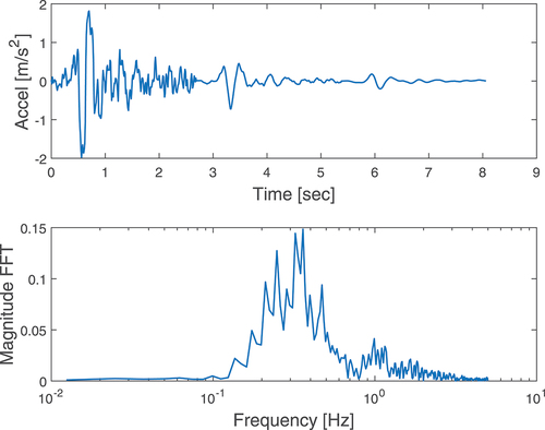
In this work, we used the accelerations of a $7.5Mw$ seism registered in 1977 by the National Institute for Earth Physics (Bucharest, Romania) (Ambraseys et al. 2002). These accelerations were multiplied by the total mass of the building to obtain ${\mathrm{\Gamma }}_1$, which is the variable required for our model. Figure 5 presents both the acceleration as a function of time and the single-sided amplitude spectrum of the acceleration.

Figure 5. Acceleration as a function of time and the single-sided amplitude spectrum of the acceleration.

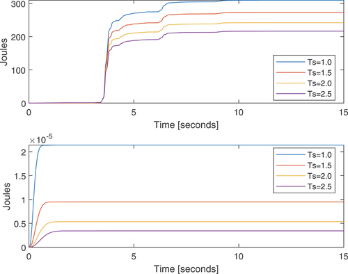
5.1. Control performance

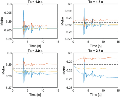
The actuators $P_5$, $P_{10}$ and $P_{15}$ counteract the movements generated by $P_1$, which simulates the seismic forces presented in Figure 5. Figure 6 shows the length of the bars for the PD control. As the value of $T_s$ increases, the structure becomes more flexible, and therefore, the bars show higher deviations from their desired values. For low values of $T_s$, the length of the bars is closer to the desired one.

Figure 6. PD control. Elongations of the diagonal bars for different values of $T_s$. The dotted line corresponds to the desired length. The graphs in blue, red and yellow correspond to the joints $q_5$, $q_{10}$, and $q_{15}$, respectively. In ALL four cases $\xi$ was set to $0.707$.

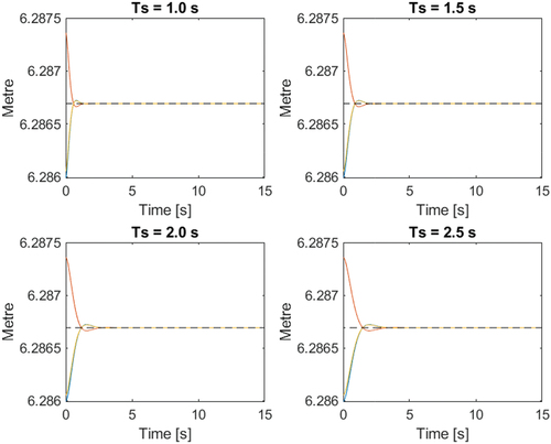
Figure 7 presents the length of the diagonal bars for the CTC control and considering the same seismic forces used for the PD. Equation (16)(16) $\left[\begin{array}{ccc}{\mathbf{A}}_r(q)& -{\mathbf{B}}_{sd}& -\mathbf{J}{(q)}^T\\ {\mathbf{J}}_r(q)& 0& 0\end{array}\right]\left[\begin{array}{c}{\ddot{q}}_r\\ {\mathrm{\Gamma }}_{sd}\\ F\end{array}\right]=\left[\begin{array}{c}{B}_1{\mathrm{\Gamma }}_1-{\mathbf{A}}_{sd}(q){\ddot{q}}_{sd}^d-H(q,\dot{q})\\ R\left(q,\dot{q}\right)-{\mathbf{J}}_{sd}(q){\ddot{q}}_{sd}^d\end{array}\right]$(16) guarantees the linearisation and decoupling between joints $q_5$, $q_{10}$, $q_{15}$, and additionally ensures that these variables are not affected by the disturbance force applied through $P_1$. Figure 7 shows that under ideal conditions (perfectly known mathematical model of the structure and exact measurement of variables), the response of system is independent of $T_s$.

Figure 7. CTC control. Elongations of the diagonal bars for different values of $T_s$. The dotted line corresponds to the desired length. The graphs in blue, red, and yellow correspond to the joints $q_5$, $q_{10}$, and $q_{15}$, respectively.In all four cases $\xi$ was set to $0.707$.

5.2. Control Efforts

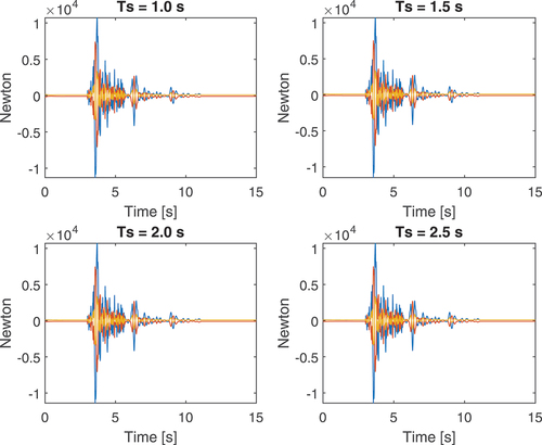
Figures 8 and 9 present the control efforts exerted by the actuators $P_5$, $P_{10}$, and $P_{15}$. These figures show that the price for the high performance of the CTC is a peak in the control effort near to the double of the peak for the PD.

Figure 8. PD control. Forces exerted by the actuators $P_5$, $P_{10}$, and $P_{15}$.

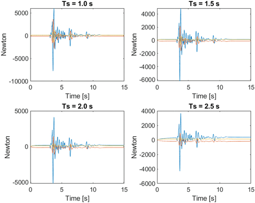
Figure 9. CTC control. Forces exerted by the actuators $P_5$, $P_{10}$, and $P_{15}$.

5.3. Energy balances

Figure 10 shows that for the PD, the energy transferred by the seism to the structure increases when the settling time $T_s$ decreases. For the CTC, this energy does not change significantly with $T_s$. From Figure 10, it can be seen that for all values of $T_s$, the PD leads to more energy absorption than the CTC.

Figure 10. Energy transferred by the seism to the structure versus time considering different values for $T_s$.

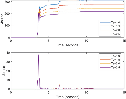
Figure 11 presents the energy dissipated for each controller. The PD dissipates much more energy than the CTC because the PD allows the seism to inject more energy into the structure than the CTC. For the PD, the dissipated energy almost equals the input energy for $t\ge 5$ seconds. It can be verified by seeing Figure 12. For the CTC, almost no energy is dissipated. This is explained by Figure 7 that shows that the length of diagonal bars remains almost constant and, as a consequence, dampers cannot transform seismic energy into heat.

Figure 11. Dissipated energy versus time for different values of $T_s$.

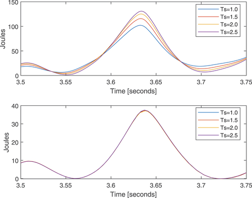
Figure 12 shows the energy stored by the structure for each controller. The main difference between the PD and the CTC occurs at $t=3$ seconds, that is when the seism occurs. The peak of energy for the PD is 120 joules, whereas the peak for the PD is 40 joules. Figure 13 is a zoom of Figure 12 around the time interval $[3.5,3.75]$ seconds that shows that the stiffer the system, the lower the maximum of energy stored by the structure. According to Figure 2, the inverse relation between stored energy and $T_s$ indicates that the frequency range where the seismic signal reaches its maximum power is below the resonance frequency of the structure.

Figure 12. Stored energy versus time for different values of $T_s$.

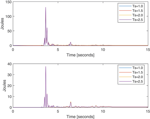
Figure 13. Stored energy versus time around the peak presented in Figure 12.

6. Conclusion and future work

In this work, the NE algorithm is used to model a three-story building with 12 revolutes and four prismatic joints and holonomic constraints. The resulting model comprises four nonlinear second-order differential equations. This modelling approach is common in robotics but has rarely been used in structural control, where most models are linear multibody mass-spring-damper systems. Our model is not only used for simulation but also to design the CTC controller. Since the simulation and control models were the same, the CTC led to a perfect linearisation and decoupling of the structure. On the other hand, in the control of a real structure, the dynamics used to synthesise the CTC will be different of the dynamics of the actual structure, and as a consequence, linearisation and decoupling will be only partially achieved. Despite the high performance of CTC with respect to the PD, the CTC is not a realistic option for structural control since it requires: (i) a detailed model of the structure, (ii) sensors for joint positions and velocities, and (iii) to measure the forces affecting the structure during an earthquake. Besides, to tune the PD only the total mass of the building is required. Future work consists of evaluating the robustness of the CTC against incertitude in the nonlinear model. This can be done through Monte-Carlo simulations, where masses, inertias, and lengths will be represented as random variables, or by implementing the CTC in real-scale structure with actuators and sensors to prove the simulation results.

The structural control system defines the settling time of a structure and, therefore, its mechanical impedance, which in turn modifies the maximum energy that the structure receives from an external source of movement. Depending on the frequency of the seismic signal, the input energy peak may increase or decrease with the settling time. On the contrary, the maximum stored energy always decreases as the settling time decreases. This relationship was verified for a linear mass-spring-damper system and for the nonlinear structure described in Section 3, but a general proof remains for future work.

Acknowledgments

The authors would like to recognise and express their sincere gratitude to Universidad del Cauca [ISNI: 0000 0001 2158 6862] (Colombia), for the financial support granted during this project.

Disclosure statement

No potential conflict of interest was reported by the author(s).

Additional information

Funding

This work was supported by the Universidad del Cauca

Notes on contributors

Carlos F. Rengifo

Carlos F. Rengifo received the degree in electrical engineering and the master’s degree in automatic control from the Universidad del Valle, Colombia, and the Ph.D. degree in robotics from the École Centrale de Nantes, France, in 2010. He is currently a Full Professor at Universidad del Cauca, Colombia. His research interests includes modeling and control of robots, and biomechanical systems.

Diego A. Bravo

Diego A. Bravo received the B.S. degree in physical engineering from the Universidad del Cauca, Colombia, in 2003, the M.S. degree in automatic engineering from the Universidad del Valle, Colombia, in 2012, and the Ph.D. degree from the Universidad del Cauca, in 2016. He is currently a Full Professor with the Physics Department at Universidad del Cauca. His research includes modeling and control of dynamical systems, and system identification.

References

- Ambraseys, N., P. Smit, R. Sigbjornsson, P. Suhadolc, and B. Margaris (2002), Internet-site for European Strong-motion Data, Technical report, European Commission, Research-Directorate General, Environment and Climate Programme.
- Åström, K., and T. Hägglund. 2006. Advanced PID Control. ISA-The Instrumentation, Systems, and Automation Society.
- Astroza, R., and A. Alessandri. 2019. “Effects of Model Uncertainty in Nonlinear Structural Finite Element Model Updating by Numerical Simulation of Building Structures.” Structural Control and Health Monitoring 26 (3): e2297. e2297 STC-17-0316.R2. doi:10.1002/stc.2297.
- Bouayed, K., M. Hamdi, and M. Rachik. 2013. “Finite Element Modelling of Sandwich Shell Structures Application to a Windscreen Panel.” Structural Control and Health Monitoring 20 (4): 593–608. doi:10.1002/stc.1480.
- Bravo, M., D. A., R., C. F. Rengifo, O. Díaz, and J. F. 2019. “Comparative Analysis between Computed Torque Control, Lqr Control and Pid Control for a Robotic Bicycle.” in 2019 IEEE 4th Colombian Conference on Automatic Control (CCAC), Medellín, (Colombia)., pp. 1–6. doi: 10.1109/CCAC.2019.8920870.
- Cao, S., H. Ouyang, and L. Cheng. 2019. “Baseline-free Multidamage Identification in Plate-like Structures by Using Multiscale Approach and Low-rank Modelling.” Structural Control and Health Monitoring 26 (2): e2293. e2293 STC-18-0093.R1. doi:10.1002/stc.2293.
- Cheng, F., and P. Tian. 1992. “Generalized Optimal Active Control Algorithm for Nonlinear Seismic Structures.” in Earthquake Engineering, Tenth World Conference, Madrid, Spain.
- Chiaia, B., G. Marasco, G. Ventura, and C. Zannini Quirini. 2020. “Customised Active Monitoring System for Structural Control and Maintenance Optimisation.” Journal of Civil Structural Health Monitoring 10: 267–282. doi:10.1007/s13349-020-00382-8.
- Cramer, N., S. S.-M. Swei, K. C. Cheung, and M. Teodorescu. 2016. “Extended Discrete-time Transfer Matrix Approach to Modeling and Decentralized Control of Lattice-based Structures.” Structural Control and Health Monitoring 23 (10): 1256–1272. doi:10.1002/stc.1837.
- Di Girolamo, G. D., F. Smarra, V. Gattulli, F. Potenza, F. Graziosi, and A. D’Innocenzo. 2020. “Data Driven Optimal Predictive Control of Seismic Induced Vibrations in Frame Structures.” Structural Control and Health Monitoring 27 (4). doi:10.1002/stc.2514.
- Dixon, J. 2007. The Shock Absorber Handbook. Wiley-Professional Engineering Publishing, 2 edn. United States: John Wiley & Sons.
- Fabien, B. C. 2008. Analytical System Dynamics: Modeling and Simulation. New York, USA: Springer.
- Gu, X., Y. Yu, J. Li, and Y. Li. 2017. “Semi-active Control of Magnetorheological Elastomer Base Isolation System Utilising Learning-based Inverse Model.” Journal of Sound and Vibration 406: 346–362. doi:10.1016/j.jsv.2017.06.023.
- Gu, X., Y. Yu, Y. Li, J. Li, M. Askari, and B. Samali. 2019. “Experimental Study of Semi-active Magnetorheological Elastomer Base Isolation System Using Optimal Neuro Fuzzy Logic Control.” Mechanical Systems and Signal Processing 119: 380–398. doi:10.1016/j.ymssp.2018.10.001.
- Güemes, A., A. Fernandez-Lopez, A. R. Pozo, and J. Sierra-Pérez. 2020. “Structural Health Monitoring for Advanced Composite Structures: A Review.” Journal of Composites Science 4 (1): 13. doi:10.3390/jcs4010013.
- Khalil, W., and E. Dombre. 2004. Modeling, Identification and Control of Robots. 2 edn ed. Butterworth - Heinemann, Paris, France: Kogan Page Science paper edition.
- Li, G., Y. Chen, C. Wen, C. Wang, J. Li, and J. Chen. 2017. “Quality Evaluation of Point Cloud Model for Interior Structure of a Common Building, in 2017 IEEE International Geoscience and Remote Sensing Symposium (IGARSS), Fort Worth, Texas, USA. pp. 6040–6043. doi: 10.1109/IGARSS.2017.8128387.
- Makisha, E. 2019. “Classification of Types of Verification for Building Information Models.” in 2019 International Multi-Conference on Industrial Engineering and Modern Technologies (FarEastCon), Vladivostok, Russian Federation, pp. 1–4. doi: 10.1109/FarEastCon.2019.8934092.
- Mohamed, A., and G. Lakhdar. 2016. “GMV Control Algorithm for Civil Engineering Structures under Bidirectional Earthquakes Using Decentralized Model.” in 2016 16th International Conference on Control, Automation and Systems (ICCAS), HICO, Gyeongju, Korea, pp. 145–150. doi: 10.1109/ICCAS.2016.7832312.
- Munteanu, R. I., G. B. Nica, V. Calofir, S. S. Iliescu, and O. T. Sirbu. 2020. “Building Seismic Behavior Improvement Using an Optimal Control Algorithm.” in 2020 IEEE International Conference on Automation, Quality and Testing, Robotics (AQTR), Cluj-Napoca, Romania, pp. 1–6. doi: 10.1109/AQTR49680.2020.9130005.
- Nambiar, K. 1969. “A Generalization of the Maximum Power Transfer Theorem.” Proceedings of the IEEE 57 (7): 1339–1340. doi:10.1109/PROC.1969.7266.
- Oviedo, J. A., and M. d. P. Duque. 2006. “Sistemas de control de respuesta sísmica en edificaciones.” Revista EIA 6: 105–120.
- Pieczonka, L., F. Aymerich, G. Brozek, M. Szwedo, W. J. Staszewski, and T. Uhl. 2013. “Modelling and Numerical Simulations of Vibrothermography for Impact Damage Detection in Composites Structures.” Structural Control and Health Monitoring 20 (4): 626–638. doi:10.1002/stc.1483.
- Reksowardojo, A. P., and G. Senatore. 2020. “A Proof of Equivalence of Two Force Methods for Active Structural Control.” Mechanics Research Communications 103: 103465. doi:10.1016/j.mechrescom.2019.103465.
- Renzi, E., and G. Serino. 2004. “Testing and Modelling a Semi-actively Controlled Steel Frame Structure Equipped with Mr Dampers.” Structural Control and Health Monitoring 11 (3): 189–221. doi:10.1002/stc.36.
- Richardson, R., M. Brown, B. Bhakta, and M. Levesley. 2005. “Impedance Control for a Pneumatic Robot-based around Pole-placement, Joint Space Controllers.” Control Engineering Practice 13 (3): 291–303. Aerospace IFAC 2002. doi:10.1016/j.conengprac.2004.03.011.
- Shih, M., and W. Sung. 2020. “Structural Control Effect and Performance of Structure under Control of Impulse Semi-active Mass Control Mechanism.” Iranian Journal of Science and Technology, Transactions of Civil Engineering 45: 1211–1226.
- Soliman, I. M., M. J. Tait, and A. A. El Damatty. 2017. “Modeling and Analysis of a Structure Semi-active Tuned Liquid Damper System.” Structural Control and Health Monitoring 24 (2): e1865. e1865 STC-14-0091.R3. doi:10.1002/stc.1865.
- Swartz, A. R. 2011. “Reduced-order Modal-domain Structural Control for Seismic Vibration Control over Wireless Sensor Networks.” in American Control Conference, San Francisco, California.
- Yan, G., H. Sun, and O. Buyukozturk. 2017. “Impact Load Identification for Composite Structures Using Bayesian Regularization and Unscented Kalman Filter.” Structural Control and Health Monitoring 24 (5): e1910. e1910 STC-16-0012.R1. doi:10.1002/stc.1910.
- Yang, Y., R. Sayed, G. Xiaoyu, L. Yancheng, L. Jianchun, and H. Quang. 2016. “Magnetorheological Elastomer Base Isolator for Earthquake Response Mitigation on Building Structures: Modeling and Second-order Sliding Mode Control.” Earthquakes and Structures 11 (6). doi:10.12989/EAS.2016.11.6.943.
- Yang, Y., R. Sayed, L. Yancheng, L. Jianchun, M. Y. Amir, G. Xiaoyu, L. Shaoqi, and L. Huan. 2020. “Dynamic Modelling and Control of Shear-mode Rotational MR Damper for Mitigating Hazard Vibration of Building Structures.” Smart Materials and Structures 29 (11): 114006. doi:10.1088/1361-665x/abb573.
- Yang, Y. W., and C. K. Soh. 2009. “2 - Piezoelectric Impedance Transducers for Structural Health Monitoring of Civil Infrastructure Systems.” In Structural Health Monitoring of Civil Infrastructure Systems, edited by V. M. Karbhari and F. Ansari, 43–71. Sawston, Cambridge: Woodhead Publishing Series in Civil and Structural Engineering, Woodhead Publishing. doi:10.1533/9781845696825.1.43.
- Zhang, C. 2014. “Control Force Characteristics of Different Control Strategies for the Wind-excited 76-story Benchmark Building Structure.” Advances in Structural Engineering 17 (4): 543–559. doi:10.1260/1369-4332.17.4.543.
- Zhang, X., W. Feng, H. Du, L. Li, S. Wang, L. Yi, and Y. Wang. 2020. “The 2018 Mw 7.5 Papua New Guinea Earthquake: A Dissipative and Cascading Rupture Process.” Geophysical Research L Etters 47 (17). doi:10.1029/2020GL089271.
- Zhang, C., L. Li, and J. Ou. 2009. “Swinging Motion Control of Suspended Structures: Principles and Applications.” Structural Control and Health Monitoring 17: 549–562. doi:10.1002/stc.331.
- Zhang, C., and J. Ou. 2015. “Modeling and Dynamical Performance of the Electromagnetic Mass Driver System for Structural Vibration Control.” Engineering Structures 82: 93–103. doi:10.1016/j.engstruct.2014.10.029.
- Zhang, C., and H. Wang. 2020. “Swing Vibration Control of Suspended Structures Using the Active Rotary Inertia Driver System: Theoretical Modeling and Experimental Verification.” Structural Control and Health Monitoring 27 (6). doi:10.1002/stc.2543.
- Zhao, H., Y. Ding, A. Li, W. Sheng, and F. Geng. 2020. “Digital Modeling on the Non- Linear Mapping between Multi-source Monitoring Data of In-service Bridges.” Structural Control and Health Monitoring 27 (11): e2618. doi:10.1002/stc.2618.
- Ziyaeifar, M., S. Gidfar, and M. Nekooei. 2012. “A Model for Mass Isolation Study in Seismic Design of Structures.” Structural Control and Health Monitoring 19 (6): 627–645. doi:10.1002/stc.459.