Performance of Value at Risk models in the midst of the global financial crisis in selected CEE emerging capital markets

Abstract

The aim of this paper is to investigate the performance of Value at Risk (VaR) models in selected Central and Eastern European (CEE) emerging capital markets. Daily returns of Croatian (CROBEX), Czech (PX50), Hungarian (BUX) and Romanian (BET) stock exchange indices are analysed for the period January, 2000 – February, 2012, while daily returns of the Serbian (BELEX15) index is examined for the period September, 2005 – February, 2012. In recent years there has been much research conducted into VaR in developed markets, while papers dealing with VaR calculation in CEE are rare. Furthermore, VaR models created and suited for liquid and well-developed markets that assume normal distribution are less reliable for capital markets in emerging economies, such as Central and Eastern European Union member and candidate states. Since capital markets in European emerging economies are highly volatile, less liquid and strongly dependent on the unexpected external shocks, market risk estimation based on normality assumption in CEE countries is more problematic. This motivates us to implement GARCH-type methods that involve time varying volatility and heavy tails of the empirical distribution of returns. We test the hypothesis that using the assumption of heavy tailed distribution it is possible to forecast market risk more precisely, especially in times of crisis, than under the assumption of normal distribution or using historical simulations method. Our backtesting results for the last 500 observations are based on the Kupiec POF and Christoffersen independence test. They show that GARCH-type models with t error distribution in most analysed cases give better VaR estimation than GARCH type models with normal errors in the case of a 99% confidence level, while in the case of a 95% confidence level it is the opposite. The results of backtesting analysis for the crisis period (after the collapse of Lehman Brothers) show that GARCH-type models with t-distribution of residuals provide better VaR estimates compared with GARCH-type models with normal distribution, historical simulations and RiskMetrics methods. The RiskMetrics method in the most cases underestimates market risk.

Keywords:

• Value at Risk (VaR)
• emerging European Economies
• GARCH models
• backtesting

JEL classifications:

• G24
• C14
• C22
• C52.

1. Introduction

Banks, investment funds and other financial institutions often use the concept of Value at Risk (VaR) as a measure of market risk. Value at risk is the assessment of the maximum potential loss in value of a portfolio over a given time horizon at a given confidence level. Based on the VaR, financial institutions are able to determine the level of capital that provides cover losses and ensures the financial position of extreme market movements.

In the global financial crisis, conditions for investors are extremely important to accurately measure and allocate risk as well as to more efficiently manage their portfolio. The influence of extreme events on the trends in financial markets in emerging countries is even more pronounced, since it is a market characterised by lower levels of liquidity and significantly smaller market capitalisation. Financial markets in emerging countries are usually characterised by a number of reforms and greater likelihood of internal and external shocks such as inflation, a sudden depreciation of national currencies, changes in credit ratings, risk premium change, etc. As this market is characterised by a greater influence of internal trade and consequently a higher degree of volatility than the markets of developed countries, the distribution of returns is significantly more distorted than normal, which makes evaluation of VaR with standard methods that assume a normal distribution of returns more difficult. Application of VaR methodology, which is basically designed and developed for liquid and developed markets, is necessary to test emerging markets that are characterised by extreme volatility, illiquidity and the shallowness of the market. Implementation of the VaR methodology in the investment process is directly related to the selection of the appropriate method of estimation. In selecting the appropriate method of key importance, it is important that it accurately determines the likelihood of losses.

The risk assessment values can be made using parametric and non-parametric methods. The historical simulation method is the best known non-parametric VaR valuation method by which a given percentile estimate is based on realised returns. A characteristic of this method is that it does not assume any specific yield distribution (normal, Student’s t-distribution, and so on), except for the invariability of distribution during the observed period. The best known method of assessing parametric VaR is a variant-covariant method, which assumes that returns follow a specific distribution, which facilitates the evaluation of the corresponding percentile. Although for simplicity of calculating VaR, researchers and investors often assume a normal distribution of returns, this assumption is usually not fulfilled in practice. The time series returns, as well as most other financial series are usually characterised by the distribution that has heavier tails than normal and by accumulation of volatility (volatility clustering). The class of GARCH-type models of conditional heteroscedasticity takes into account these properties of financial series and provides a more accurate VaR estimate.

This paper will test the applicability of the concept of VaR to the markets of selected countries in Central and Eastern Europe (Czech Republic, Hungary, Croatia, Romania and Serbia). A particular challenge is the possibility of using VaR in the financial markets of countries in transition. Although different in certain aspects, these countries have similarities since all of them recently joined the EU or acceded to the integration process (Serbia). In addition, all countries are emerging markets and provide investment opportunities for those investors who wish to diversify their portfolios. The analysis used stock index PX50 (Prague Stock Exchange), BUX (Budapest Stock Exchange), BELEX15 (Belgrade Stock Exchange), CROBEX (Zagreb stock exchange), and BET (Bucharest Stock Exchange). Given the recession business environment, the results of research will be, in particularly, interesting to domestic and foreign investors. In addition, the results are relevant to the macro (social, economic, political, etc.) and the microeconomic level (enterprise).

This paper is structured as follows. The literature review is presented in the second section. Section three describes the methodology employed. The fourth section presents the results of empirical analysis and backtesting. Finally, concluding remarks are given in the fifth section.

2. Literature review

Almost all researchers are unanimous that there is no single approach or a VaR model that is optimal in all markets and in all situations. According to previous published studies, VaR models based on moving averages give a good prediction of market risk. However, results vary depending on the loss function that was used, the chosen level of confidence VaR, the period for which the survey was conducted (turbulent or normal), the model used for assessing the VAR and so on.

In a number of papers, VaR was evaluated for developed market economies, using similar methodology to ours (for instance, Degiannakis, 2004; Linsmeier & Pearson, 2000; Duffie & Pan, 1997; Wong, Cheng, & Wong, 2002; Guermat & Harris 2002; Alexander & Leigh, 1997; Christoffersen, Hahn, & Inoue, 2001; Su & Knowles, 2006).

Although there are a number of papers relating to the testing of different models of VaR and market risk management in developed and liquid markets, a number of papers relating to testing VaR models in less developed and less liquid markets are more limited (for instance Zivkovic, 2007; Bao, Lee, & Saltoglu, 2006; Andjelic, Djokovic, & Radisic, 2010; Kavussanos, Dimitrakopoulos, & Spyrou, 2010; Thupayagale, 2010; Nikolic-Djoric & Djoric, 2011; Degiannakis, Floros, & Livada, 2012; Mutu, Balogh, & Moldovan, 2011).

For instance, Zivkovic (2007) investigated whether the VaR model (historical simulations model, a parametric variance-covariance approach, historical simulation, RiskMetrics system and variance-covariance approach using GARCH forecasts) is applicable to volatile capital markets, and the new member and candidate states (Bulgaria, Romania, Croatia and Turkey). The results point to the fact that VaR models, which are commonly used in developed capital markets, are not successful in measuring market risk in the new member and candidate states, given that returns are characterised by heavier tails, asymmetry and heteroscedasticity, which complicates estimates of VaR.

Andjelic et al. (2010) investigated the performance of VaR models (parametric and historical simulation models) on a sample of daily stock index returns of four different capital markets of developing countries (Slovenia, Croatia, Serbia and Hungary) with a confidence interval of 95% and 99%. The results indicate that the studied models give good predictions of market risk with a 95% confidence interval in stable market conditions, while in the case of volatile market conditions tested models with 99% confidence interval give good estimates of market risk. They suggest that models that give an accurate assessment of the value of VaR in developed markets may not achieve the same results in developing and illiquid capital markets.

Nikolic-DJoric and DJoric (2011) used RiskMetrics, GARCH and IGARCH models to calculate daily VaR Belgrade Stock Exchange index BELEX15 returns based on normal and Student’s t-distribution. In addition, authors applied extreme value theory (EVT) on standardised residuals. The results indicate that since the returns of BELEX 15 index are characterised by volatility clustering, the use of GARCH models in combination with the POT method reduces the average value of VaR. In addition, the authors conclude that IGARCH models cannot outperform GARCH models.

Mutu, Balogh, and Moldovan (2011) analysed the performance of some VaR models (historical simulation, EWMA, GARCH and EVT) on daily data of five Eastern and Central European main indices: BET (Romania), PX50 (Czech Republic), BUX (Hungary), SOFIX (Bulgaria) and WIG20 (Poland) from 2004 to 2009. In order to highlight different behaviours in the crisis period, authors divided the data into two samples and found that EVT and GARCH models can adequately measure the risk of the capital markets and satisfy the requirements of the investors in periods characterised by extreme events.

3. Methodology

3.1. Defining the concept of Value at Risk (VaR)

VaR is a measure that gives the maximum potential loss that can be realised from certain investments over a given time horizon (usually 1 day or 10 days), with a certain probability (Jorion, 2001). Mathematically, VaR for the period of the k day in day t can be represented as follows:(1)

where P_t is the price of a particular type of financial asset, and α represents a given level of probability.

VaR can be expressed in terms of a percentile of the return distributions. Specifically, if is the th percentile of the continuously compound return, VaR is calculated as follows:(2)

The previous equation implies that a good estimate of VaR can only be produced with an accurate forecast of the percentiles, , which is obtained on the corresponding volatility modelling. Therefore, we discuss below the value of VaR for a series of returns.

Define a one-day return on day t as:(3)

For the time series of return , VaR can be expressed as:(4)

From this equation it follows that finding the VaR values is ​​the same as finding a 100α% conditional quintile. Formally, it is possible to develop models for the stock returns as follows:(5)

where is a set of information available at time , and where and are functions of a certain dimensional vector of parameter values . In this model, is innovation, is the unobserved volatility, and is the martingale difference sequence satisfying:(6)

As a consequence, we have:(7)

where represents the conditional distribution with zero mean value and variance .

If the return can be modelled by a parametric distribution, VaR can be derived from the distributional parameters. Unconditioned parametric models were determined with and . Therefore, we assume that returns are independent and equally distributed with a given density function:(8)

where is the density function of distribution of r_t and is the density function of the standardised distribution of .

Below, we present the most commonly used parametric and non-parametric models that enable VaR estimates, the exponentially weighted moving average model (EWMA), historical simulations model (HS) and the conditional volatility models (GARCH type models).

3.2. Historical simulations model

The historical simulation model (HS) of VaR calculation does not use the assumption of certain types of distributions, but uses actual data from the past (Barone-Adesi & Giannopoulos, 2001). The main advantage of historical simulation is non-parametrical or the non-existence of assumptions regarding the distribution of portfolio returns. The only assumption is that the returns are independently and identically distributed (iid). This assumption is based on the market efficiency theory that the returns are periodically mutually uncorrelated, this means that the return of one period does not depend on the return of the previous period. If price changes depend only on the new information, which means that they cannot be predicted, then they will be time uncorrelated (Neftci, 2004).

A problem with HS is that owing to discreteness of extreme returns and very few observations in the tails, the VaR measures are expected to be highly volatile and erratic (Meera, 2012). Danielsson and De Vries (1997) observe that the under/over prediction of VaR by HS is more severe in the case of an individual stock than an index. The underlying assumption in a HS, that returns are iid, is another problem with the approach, making VaR estimates unresponsive to recent innovations in volatility. Modifications to the HS have aimed at bettering the problem of discreteness of extreme returns and the low responsiveness to recent volatility. Boudoukh, Richardson, and Whitelaw (1998) modify the historical simulation approach by assigning exponentially declining weights (as in EWMA) to the most recent observations (HSWT). Hull and White (1998) improve the historical simulation method by altering it to incorporate volatility updating. They adjust the returns in the historical sample with the ratio of the current daily volatility to the historical volatility, both estimated using a conditional volatility model such as GARCH or EWMA (Hull & White, 1998, use EWMA with λ = 0.94). This altered method (modifying HS with GARCH) – called the filtered historical simulation (FHS) by Barone-Adesi, Giannopoulos, and Vosper (1999) – effectively makes the HS more responsive to current data.

3.3. The exponentially weighted moving average model (EWMA)

Since the JP Morgan 1994th RiskMetrics model was developed to measure VaR, VaR calculated in this way becomes a benchmark measure of market risk in practice. The starting assumption of the RiskMetrics model is that returns of a certain type of financial assets have a conditional normal distribution with arithmetic mean zero and variance expressed as the value of the exponential weighted moving average historical rate of ​​squared values of return. However, in practice, it was confirmed that the distribution of returns of financial assets generally deviates from the normal, i.e. has heavier tails, so the assessments of VaR obtained by this model are biased. Second, in many empirical studies (see for example Ding, Granger, & Engle, 1993; So, 2000) it was observed that returns of different types of financial assets are characterised by long memory, which is reflected in the assessment and prediction of market volatility.

RiskMetrics’ VaR model evaluation assumes a dynamic model of exponentially weighted moving average (EWMA) of the variance:(9)

In order to initialise a recursive equation of variance, the sampling variance is used:(10)

where, following RiskMetrics system, the value of the parameter λ is 0.94 for daily data and 0.97 for monthly data. The parameter is called a smoothing parameter, which determines the exponentially declining weighting scheme of the observations. The smaller , the greater the weight is given to recent return data. An exponentially weighted moving average model can be represented as:(11)

If it is assumed that the conditional distribution of returns is normal with mean value zero and variance , then the one-day VaR on day t is obtained as follows:(12)

where is 100α percent of N(0,1), respectively is the inverse distribution function of a standardised normal random variable.

However, if returns are characterised by Student’s t-distribution with mean value zero, then the value of one-day VaR is calculated as:(13)

where is the left quintile at α% and t is the distribution function for the Student’s t-distribution with the estimated number of degrees of freedom v.

3.4. GARCH-type models

The GARCH-type model successfully captures several characteristics of financial time series, such as thick-tailed returns and volatility clustering. This type of model represents a standard and very often used approach for obtaining a VaR estimate. A general GARCH(p,q) model proposed by Bollerslev (1986) can be written in the following form:(14)

The first equation actually describes the percentage level of return, which is presented in the form of autoregressive and moving average terms, i.e. the ARMA (m,n) process. Error term in the first equation is a function of , which is a random component with the properties of white noise. The third equation describes the conditional variance of return, , which is a function of q previous periods and conditional variance of p previous periods. The stationarity condition for GARCH (p, q) is .

The size of parameters and in the equation determines the observed short-term volatility dynamics obtained from the series of returns. The high value of coefficient indicates that shocks to conditional variance need a long time to disappear, so the volatility is constant. The high value of the coefficient means that volatility reacts intensively to changes in the market.

If , for sufficiently long horizon forecasts, the conditional variance of the GARCH(p, q) process than converges to:

(15)

is called the unconditional variance of GARCH (p, q) process.

By standard arguments, the model is covariance stationary if and only if all the roots of lie outside the unit circle. In many applications with high frequency financial data the estimate for turns out to be very close to unity. This provides an empirical motivation for the so-called integrated GARCH(p,q), or IGARCH(p,q), model (see Bollerslev, Engle, & Nelson, 1994)]. In the IGARCH class of models, the autoregressive polynomial in equation (14(14) ) has a unit root, and consequently a shock to the conditional variance is persistent in the sense that it remains important for future forecasts of all horizons. A general IGARCH (p, q) process can be written in the following form:(16)

where A(L) and B(L) are lag operators.

In order to capture asymmetry, Nelson (1991) proposed an exponential GARCH processor EGARCH for the conditional variance:(17)

An asymmetric relation between returns and volatility change is given as function which represents the linear combination of and :

(18)

where and are constants.

By construction, equation (18) is a zero mean process (bearing in mind that ). For , is a linear function with slope coefficient  + γ, while for - < it is a linear function with slope coefficient . The first part of the equation, , captures the size effect, while the second part, , captures the leverage effect.

Zakoian (1994) proposed a TGARCH (p,q) model as an alternative to the EGARCH process, where the asymmetry of positive and negative innovations is incorporated in the model by using the indicator function:(19)

where are parameters that have to be estimated, d(·) denotes the indicator function defined as:(20)

The TGARCH model allows good news, and bad news, to have differential effects on the conditional variance. For instance, in the case of the TGARCH (1,1) process, good news has an impact of α₁, while bad news has an impact of α₁ + γ₁. For γ₁ > 0, the leverage effect exists.

The APARCH (p, q) process, proposed by Ding, Granger, and Engle (1993), includes seven different GARCH-type models (ARCH, GARCH, AGARCH, TGARCH, TARCH, NGARCH and Log-GARCH):(21)

where and Parameter in the equation denotes the exponent of conditional standard deviation, while parameter describes the asymmetry effect of good and bad news on conditional volatility. The positive value of means that negative shocks from previous period have a higher impact on the current level of volatility, and otherwise.

Based on estimated parameters of the GARCH-type process it is possible to make a forecast of and conditional volatility for the next k periods (for details see Mladenovic & Mladenovic, 2006)]. The forecasted value of return and the conditional volatility for the next period are obtained as follows:(22)

If residuals follow standardised normal distribution, the VaR at 95% confidence level could be calculated as:(23)

while if residuals follow standardised distribution with v degrees of freedom, then the VaR could be calculated as:(24)

3.5. Backtesting

Backtesting represents a statistical procedure by which losses and gains are systematically compared with the appropriate valuation of VaR. In the backtesting process it can be statistically examined if the frequency exceptions, during the selected time interval, are in accordance with the chosen confidence level. These types of tests are known as tests of unconditional coverage. The most famous test in this group is the Kupiec test.

In theory, however, a good VaR model not only shows the correct amount of exceptions, but exceptions that have been evenly distributed over time, i.e. that are independent from each other. The grouping of exemptions indicates that the model does not register changes in the market volatility and correlation in the correct manner. The conditional coverage test, therefore, examines conditionality and changes in data over time (Jorion, 2001). The most commonly used test of this group is the Christoffersen independence test.

The Kupiec test

The Kupiec test, known as the proportions of failures test (POF), measures whether the number of exemptions is consistent with a given confidence level (Kupiec, 1995). If the null hypothesis is true, then the number of exemptions follows the binomial distribution. Therefore, to implement the POF test it is necessary to know the number of observations (n), the number of exceptions (x) and the confidence level.

The null hypothesis of the POF test is:

The basic idea is to determine if the observed excess rate is significantly different from p, the excess rate determined by the given confidence level. According to Kupiec (1995), the POF test is best implemented as a likelihood-ratio test (LR). The statistical test has the following form:(25)

If the null hypothesis is correct, statistics in asymptotic conditions have a distribution with a single degree of freedom. If the value of statistics exceeds the critical value of distribution, the null hypothesis is rejected and the model is considered to be imprecise.

The Christoffersen independence test

Christoffersen (1998) uses the same idea of the credibility test as Kupiec, but extends the test by introducing separate statistical values for independent exceptions. In addition, this test observes if the probability of exceptions on any day depends on the outcome of the previous day.

Let be defined as the number of days when an outcome j occurs assuming that event i occurred on the previous day. In addition, let π_i represent the probability of observing an exception conditional on state i on the previous day (Nieppola, 2009):

If the model is correct, the exception that occurs today should not depend on the exception that occurred on the previous day. In other words, if the null hypothesis is true, probabilities π₀ and π₁ should be equal.

The independence test of the exceptions is best implemented as a likelihood-ratio test (LR). The statistical test has the following form:(26)

Combining Christoffersen independence test and Kupiec POF test we get a combined test (conditional coverage test) that observes both characteristics of the VaR model, the correct rate of excess and independent exceptions:

also has an asymptotically distribution, but in this case with two degrees of freedom given that it is based on two separate LR statistics. If the value is lower than the appropriate critical value of the distribution, the model passes the test. On the contrary, the value of the statistic being greater than the critical value implies that the model is rejected.

Christoffersen’s framework allows for observing whether the reasons for not passing the test are due to inadequate coverage, clustering of exceptions or a combination of both. Evaluation is done by calculating the statistics and separately with the use of a distribution with one degree of freedom as a critical value of both statistics. In special cases it is possible for the model to pass the joint test while still failing each of the individual tests (Campbell, 2005). Therefore, separate testing is recommended even in cases when the joint test gives positive results.

4. Data and results

The research sample comprises daily returns of stock indices of selected CEE countries, which are: Hungary, Czech Republic, Romania, Croatia, and Serbia. The tested stock indices are BET, PX50, BUX, CROBEX, during the period January, 2001 – February, 2012, and BELEX15 during the period September, 2005 – February, 2012, respectively. The data are obtained from national stock exchange websites. For all indices, we compute daily logarithmic returns, i.e. r_t = (log P_t – log P_t–1) × 100. Bearing in mind that the one-time structural breaks may lead to erroneous statistical conclusions, in all five cases we indicate the most prominent non-standard values and then regress the series of returns on constant and dummy variables that take non-zero values for the observations with the most prominent non-standard values. New adjusted series of daily returns are used in empirical analysis (see Figure 1). Volatility clustering is clearly visible in all cases.

Figure 1. Stock Exchange indices daily log returns.

Source: National stock exchanges.

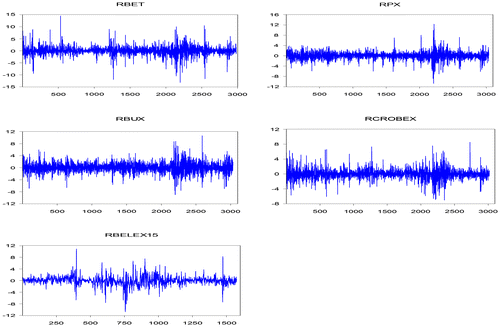
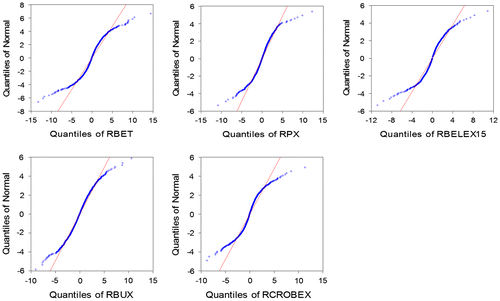
Table 1 indicates that the daily returns of all five market stock indices are not normally distributed. In most cases skewness is evident; kurtosis is in all cases much greater than 3 and the Jarque-Bera statistics are highly significant. For instance, PX50 and BET indices have highly negatively skewed distributions. The results confirm the presence of fat tails, which suggest that the assumption of a normal distribution is not satisfied and that methods that suppose normal distribution could seriously underestimate the VaR value. These findings are consistent with the normal Q-Q and empirical Q-Q plot (Figure 2). From Figure 2 it is clear that the QQ plot is not linear and that empirical distribution differs from the hypothesised normal distribution.

Table 1. Descriptive characteristics of stock exchange indices daily returns.

	Skewness	Kurtosis	JB	Q^2 (10)	Q^2 (30)	ARCH-LM (10)	ARCH-LM (30)
BUX	0.038	6.011	1146.2 (0.00)	691.94 (0.00)	1476.0 (0.00)	318.345 (0.00)	421.98 (0.00)
PX50	−0.149	9.096	4715.8 (0.00)	187.9 (0.00)	3270.4 (0.00)	661.99 (0.00)	737.06 (0.00)
BELEX15	−0.039	10.549	3779.8 (0.00)	577.46 (0.00)	786.06 (0.00)	336.73 (0.00)	361.34 (0.00)
CROBEX	0.069	9.784	5791.8 (0.00)	597.87 (0.00)	1082.2 (0.00)	310.46 (0.00)	380.30 (0.00)
BET	−0.168	10.42867	6853.7 (0.00)	646.32 (0.00)	1014.6 (0.00)	360.58 (0.00)	387.87 (0.00)

Notes: p values of corresponding test statistics are given in parentheses. JB represents Jarque-Bera statistics for normality testing, Q² represents Box-Ljung statistics for testing autocorrelation in squared standardised residuals, while the ARCH-LM test is a test of autoregressive conditional heteroscedasticity.

Source: Author’s calculations.

Figure 2. Q-Q Plot of returns.

Source: Author's calculations.

The ARCH-LM test indicates the presence of time varying volatility, and Box-Ljung statistics indicate evidence of autocorrelation in squared standardised residuals.

As the Box-Ljung autocorrelation test for squared standardised residuals and ARCH/LM tests indicate the presence of ARCH effects, we estimate models of conditional autoregressive heteroscedasticity (GARCH type models). Model selection was done according to modified Akaike criteria. Model parameters are calculated using the maximum likelihood estimation method. The maximum likelihood estimates of the parameters are obtained by numerical maximisation of the log-likelihood function using the BHHH algorithm. Estimates of parameters from different specifications of conditional heteroscedasticity models (GARCH, EGARCH, TGARCH and APARCH) together with associated tests of residual autocorrelation, normality and conditional heteroscedasticity are given in Tables A1–A10 in the Appendix.

Based on estimated parameters by GARCH-type models we get one, five and ten days ahead VaR estimates at 95% and 99% coverage of the market risk. In order to highlight differences between VaR estimates we have calculated the risk measure through historical simulation time weighted (HSWT) and EWMA models.

The results given in Tables A1 and A2 in the Appendix show that returns of stock index BET best describes the EGARCH (1,1) model, regardless of whether it is assumed that the residuals follow normal distribution or Student’s t-distribution. In the mean equation, the autoregression component of the first order is significant, i.e. the AR (1) component.

The obtained VaR values can be significantly different depending on the assumptions that the residuals follow a normal or Student’s t-distribution. The VaR measure at 99% confidence level is higher within the assumption that residuals follow Student’s t-distribution, while at the 95% confidence level it is the opposite. The application of historical simulation and EWMA methods gives a lower estimate of loss with respect to the GARCH-type methods in the case of the BET index. Based on estimated results, the maximum daily loss for the BET index daily returns ranges from €133 to €243 euros on an invested €10,000 at the 95% confidence level (Table 2).

Table 2. Estimation of the VaR for 1, 5 and 10 days ahead period for BET index returns.

	HSWT	Normal distribution	Student’s t-distribution
		GARCH (1,1)	EWMA (λ = 0.9)	EGARCH (1,1)	GARCH (1,1)	EGARCH (1,1)
VaR (1, 0.95)	1.326	2.424	1.924	2.43	2.218	2.246
VaR (1, 0.99)	1.741	3.423	2.717	3.389	3.705	3.750
VaR (5, 0.95)	2.965	5.420	4.302	5.367	4.960	5.022
VaR (5, 0.99)	3.893	7.654	6.075	7.578	8.285	8.385
VaR (10, 0.95)	4.194	7.665	6.084	7.589	7.014	7.102
VaR (10, 0.99)	5.505	10.824	8.592	10.717	11.716	11.859

Source: Author’s calculations.

In order to test the validity of the VaR estimates for one day ahead, Kupiec and Christoffersen tests were implemented for 95% and 99% confidence levels. If we compare the number of exemptions exceeding the last 500 data returns BET index, it can be concluded that the assessed VaR for GARCH-type models is adequate for 95% according to the Kupiec test, but not for the 99% confidence level (Table 3).

Table 3. Backtesting results for BET index daily returns.

	HSWT	Normal distribution			Student’s t-distribution
		GARCH (1,1)	EWMA (λ=0.9)	EGARCH (1,1)	GARCH (1,1)	EGARCH (1,1)
Kupiec test 95%	47.684*	2.277	2.459	2.277	0.172	0.710
Kupiec test 99%	121.07*	10.994*	17.902*	10.994*	7.11*	7.11*
Christoffersen test 95%	11.787*	5.171*	5.539*	5.171*	6.226*	7.629*
Christoffersen test 99%	5.780	22.628*	21.836*	22.628*	10.017*	10.017*

Source: Author’s calculations.

PX50 stock index returns best describe the APARCH (1,1) model, regardless of whether it is assumed that the residuals have a normal distribution or the Student’s t-distribution. In the mean equation, the autoregression component of the first order is significant, but the estimated value of the autoregression parameter is very small. Maximum daily loss for the PX50 index daily returns ranges from €212 to €256 on an invested €10,000 at 95% confidence level. Predicted VaR varies depending on the assumed specification of conditional variance, especially for the 99% confidence level (Table 4).

Table 4. Estimation of the VaR for 1, 5 and 10 days ahead period for PX50 index returns.

	HSWT	Normal distribution	Student’s t-distribution-
		GARCH (1,1)	APARCH (1,1)	EWMA (λ = 0.9)	GARCH (1,1)	APARCH (1,1)
VaR (1, 0.95)	2.122	2.437	2.163	2.561	2.388	2.144
VaR (1, 0.99)	2.828	3.472	3.072	3.617	3.717	3.299
VaR (5, 0.95)	4.744	5.449	4.837	5.727	5.340	4.794
VaR (5, 0.99)	6.323	7.764	6.869	8.088	8.311	7.377
VaR (10, 0.95)	6.709	7.706	6.840	8.099	7.552	6.780
VaR (10, 0.99)	8.943	10.979	9.715	11.438	11.754	10.432

Source: Author’s calculations.

The GARCH (1,1) and APARCH (1,1) models used for calculating VaR with the 95% confidence level according to the Kupiec test seems to be adequate if we assume both normal and Student’s t-distribution of returns (see Table 5). At the same time, GARCH (1,1) and APARCH (1,1) with the t-distribution of residuals are an adequate measure of market risk with the 99% confidence level according to the Christoffersen test. For the Czech market the best model that reflect the risk was GARCH (1,1) with Student’s t-distribution of residuals.

Table 5. Backtesting results for PX50 index daily returns.

	HSWT	Normal distribution			Student’s t-distribution
		GARCH (1,1)	APARCH (1,1)	EWMA (λ = 0.9)	GARCH (1,1)	APARCH (1,1)
Kupiec test 95%	0.042	2.276	0.042	2.276	1.646	0
Kupiec test 99%	10.994*	7.111*	7.111*	7.111*	2.612	7.111*
Christoffersen test 95%	14.633*	9.283*	13.431*	9.283*	8.431*	15.758*
Christoffersen test 99%	3.710	4.868	4.868	4.868	0.329	4.867

Source: Author’s calculations.

* Denotes statistical significance of the test statistics.

The BUX stock index returns best describes the TGARCH (1,1) model, regardless of whether it is assumed that the residuals have a normal distribution or a Student’s t-distribution. The BUX stock index returns characterise neither the AR nor the MA component (Table 6).

Table 6. Estimation of the VaR for 1, 5 and 10 days ahead period for BUX index returns.

	HSWT	Normal distribution			Student’s t-distribution
		GARCH (1,1)	TGARCH (1,1)	EWMA (λ = 0.94)	GARCH (1,1)	TGARCH (1,1)
VaR (1, 0.95)	2.52	2.54	2.26	2.64	2.51	2.25
VaR (1, 0.99)	3.14	3.59	3.19	3.73	3.83	3.41
VaR (5, 0.95)	5.64	5.68	5.05	5.90	5.61	5.03
VaR (5, 0.99)	7.03	8.03	7.13	8.34	8.56	7.62
VaR (10, 0.95)	7.97	8.04	7.14	8.35	7.93	7.12
VaR (10, 0.99)	9.94	11.35	10.08	11.79	12.10	10.77

Source: Author’s calculations.

However, according to the Kupiec and Christoffersen test, the GARCH(1,1) model with a normal distribution of standardised residuals and the EWMA model provide the most adequate VaR estimate (Table 7).

Table 7. Backtesting results for BUX index daily returns.

	HSWT	Normal distribution			Student’s t-distribution
		GARCH (1,1)	TGARCH (1,1)	EWMA (λ = 0.94)	GARCH (1,1)	TGARCH (1,1)
Kupiec test 95%	3.081	3.081	12.518*	1.903	4.511*	12.517*
Kupiec test 99%	10.994*	3.914	8.973*	2.613	1.538	5.419
Christoffersen test 95%	4.993*	4.993*	4.276*	1.720	4.003*	4.276*
Christoffersen test 99%	0.807	0.408	0.694	0.330	0.260	0.495

Source: Author’s calculations.

^* Denotes statistical significance of the test statistics.

The CROBEX stock index returns best describes the GARCH (1,1) and APARCH (1,1) models with the assumption that the residuals follow the normal distribution, and the GARCH (1,1) model with the assumption that the residuals follow the Student’s t-distribution. In the mean equation, the autoregression component of the first order and the component of the moving average of the first order are significant. Based on estimated results, it could be concluded that the maximum daily loss for the CROBEX index daily returns ranges from €98 to €175 on an invested €10,000 at the 95% confidence level (Table 8).

Table 8. Estimation of the VaR for 1, 5 and 10 days ahead period for CROBEX index returns.

	HSWT	Normal distribution			Student’s t-distribution
		GARCH (1,1)	APARCH (1,1)	EWMA (λ = 0.93)	GARCH (1,1)
VaR (1, 0.95)	1.75	1.27	1.33	0.98	1.16
VaR (1, 0.99)	1.88	1.81	1.88	1.39	2.03
VaR (5, 0.95)	3.91	2.85	2.97	2.20	2.59
VaR (5, 0.99)	4.19	4.06	4.19	3.10	4.55
VaR (10, 0.95)	5.52	4.03	4.20	3.11	3.66
VaR (10, 0.99)	5.93	5.74	5.93	4.38	6.44

Source: Author’s calculations.

Backtesting results show that the GARCH (1,1) specification that assumes a t-distribution of standardised returns is a superior measure of market risk for CROBEX compared with GARCH-type specifications that assume the normal distribution of residuals. The EWMA method underestimates market risk (Table 9).

Table 9. Backtesting results for CROBEX index daily returns.

	HSWT	Normal distribution			Student’s t-distribution
		GARCH (1,1)	APARCH (1,1)	EWMA (λ = 0.93)	GARCH (1,1)
Kupiec test 95%	6.018*	5.317*	0.992	32.162*	12.518*
Kupiec test 99%	10.050*	5.419	2.613	41.291*	1.54
Christoff. test 95%	0.8067	1.826	4.61*	5.07*	2.57
Christoff. test 99%	0.330	0.496	0.409	26.47*	0.101

Source: Author’s calculations.

^* Denotes statistical significance of the test statistics.

The BELEX15 stock index returns best describes the EGARCH (1,1) model with assumption that the residuals follow the normal distribution and the GARCH (1,1) model with assumption that the residuals follow the Student’s t-distribution. In the mean equation, the autoregression component of the first order and the component of moving average of the first order are significant.

Based on estimated results, it could be concluded that the maximum daily loss for the BELEX15 index daily returns ranges from €113 to €154 on an invested €10,000 at the 95% confidence level. The predicted value at risk does not significantly change depending on the assumed specification of conditional variance (Table 10).

Table 10. Estimation of the VaR for 1, 5 and 10 days ahead period for BELEX15 index returns.

	HSWT	Normal distribution			Student’s t-distribution
		GARCH (1,1)	EGARCH (1,1)	EWMA (λ = 0.87)	GARCH (1,1)
VaR (1, 0.95)	1.538	1.238	1.308	1.178	1.133
VaR (1, 0.99)	1.557	1.789	1.885	1.664	1.893
VaR (5, 0.95)	3.439	2.770	2.924	2.634	2.533
VaR (5, 0.99)	3.482	4.000	4.215	3.721	4.232
VaR (10, 0.95)	4.863	3.918	4.136	3.725	3.583
VaR (10, 0.99)	4.924	5.657	5.961	5.262	5.986

Source: Author’s calculations.

Only the historical simulation model passes the Kupiec test with the 95% confidence level (see Table 11). On the other hand, the GARCH (1,1) and EGARCH (1,1) models with normal distribution of residuals passed the Christoffersen test with the 95% confidence level. The GARCH (1,1) model that supposes Student’s t-distribution underestimates VaR at the 95% confidence level.

Table 11. Backtesting results for BELEX15 index daily returns.

	HSWT	Normal distribution			Student’s t-distribution
		GARCH (1,1)	EGARCH (1,1)	EWMA (λ = 0.87)	GARCH (1,1)
Kupiec test 95%	3.23	15.08*	11.47*	19.07*	23.42*
Kupiec test 99%	35.32*	23.52*	19.92*	23.52*	19.92*
Christoffersen test 95%	2.11	3.60	2.85	4.26*	4.83*
Christoffersen test 99%	2.69	5.02	6.05	5.02	6.05

Source: Author’s calculations.

^* Denotes statistical significance of the test statistics.

In order to compare the market risk assessment based on the historical simulations, EWMA and GARCH type models, backtesting analysis is conducted for five- and ten-days ahead estimated VaR. In the cases of BET, PX50 and the BUX index, the GARCH-type methods provide more adequate measures of VaR compared with RiskMetrics or historical simulation methods, while in the case of CROBEX, the historical simulations model better reflects market risk. In the case of BELEX15, all estimated models underestimate market risk (Table 12).

Table 12. Backtesting results for 5 and 10 days returns.

	VAR(5)				VAR(10)
	HSWT	EWMA	GARCH normal distrib.	GARCH t-distrib.	HSWT	EWMA	GARCH normal distrib.	GARCH t-distrib.
BET
Kupiec test 95%	33.97*	1.90	1.13	0.39	58.55*	9.11*	0.00	0.16
Kupiec test 99%	78.07*	20.46*	13.16*	5.42	144.48*	20.46*	8.97*	3.91
PX50
Kupiec test 95%	0.04	3.88*	0.04	0.04	95.64*	2.28	0.36	0.99
Kupiec test 99%	8.97*	1.54	1.54	3.91	15.47*	1.54	8.97*	5.42
BUX
Kupiec test 95%	0.99	0.63	0.99	4.51*	0.64	0.16	0.16	2.46
Kupiec test 99%	25.91*	13.16*	13.16*	15.47*	10.99*	5.42	5.42	7.11*
CROBEX
Kupiec test 95%	0.71	30.39*	6.18*	20.65*	0.36	80.17*	13.75*	35.81*
Kupiec test 99%	13.16*	78.07*	13.16*	8.97*	34.86*	116.53*	34.86*	7.11*
BELEX15
Kupiec test 95%	25.73*	105.21*	72.25*	25.72*	59.06*	137.99*	90.03*	142.29*
Kupiec test 99%	104.96*	77.82*	35.32*	104.96*	177.92*	152.50*	104.96*	99.36*

Source: Author’s calculations.

^* Denotes statistical significance of the test statistics.

Analysis was conducted separately for the period September 2008 – December 2009, bearing in mind that the financial markets in CEE have hardly been hit by the world financial crisis after the collapse of Lehman Brothers. This analysis was done in order to highlight the different behaviour of the market risk in the crisis period and to test the hypothesis that using the assumption of a heavy-tailed distribution it is possible to forecast market risk more precisely, especially in times of crisis, compared with using the assumption of normal distribution or using a historical simulations method.

The results of the analysis suggest the following conclusions. The GARCH model provides the most accurate volatility estimation in the case of the BUX index and the BET index with a t-distribution of the standardised residuals, TGARCH in the case of the BET and CROBEX indexes with a normal distribution of the standardised residuals, while the EGARCH model provides the best fit in other cases. VaR estimates obtained by GARCH-type models for the crisis period are higher for all capital markets except the Czech market (Table 13).

Table 13. VaR estimates for the crisis period.

	HSWT	Normal distribution			Student’s t-distribution
		EWMA	GARCH (1,1)	EGARCH/TARCH/APARCH	GARCH (1,1)	EGARCH/TARCH/APARCH
BET
VaR (1,95)	2.87	2.70	3.05	2.84	3.04	2.85
VaR (1,99)	5.09	3.81	4.31	4.01	4.69	4.44
PX50
VaR (1,95)	1.87	1.50	1.98	1.94	1.98	1.95
VaR (1,99)	4.11	2.14	2.79	2.74	3.02	2.91
BUX
VaR (1,95)	2.85	2.26	2.63	2.65	2.59	2.61
VaR (1,99)	3.40	3.19	3.71	3.75	3.87	3.89
CROBEX
VaR (1,95)	1.54	1.31	1.76	1.67	1.64	1.54
VaR (1,99)	2.51	1.85	2.49	2.37	2.89	2.72
BELEX15
VaR (1,95)	2.27	0.93	1.46	1.29	1.39	–
VaR (1,99)	2.57	1.32	2.08	1.84	2.21	–

Source: Author’s calculations.

Results of backtesting analysis for last 200 observations during the crisis period show that GARCH-type models with a t-distribution of residuals provide better VaR estimates compared with GARCH-type models with a normal distribution, historical simulations and RiskMetrics methods.

5. Concluding remarks

This paper evaluates the performance of a variety of symmetric and asymmetric GARCH-type models based on the normal and Student’s t-distributions in estimating and forecasting market risk in selected emerging economies from Central and Eastern Europe. The growing interest of foreign investors to invest in CEE financial markets and the increased fragility in these markets in times of crisis highlighted the importance of adequate market risk quantification and prediction.

Estimates obtained by our calculation imply that the considered countries were characterised by a different level of market risk, especially when a 99% confidence level is chosen. Thus, adequate VaR estimations need careful modelling of each index return series individually.

The results of backtesting show that such a GARCH-type VaR assuming a t-distribution of standardised returns in most cases is a superior measure of the downside risk at the 99% confidence level, while models with a normal distribution of residuals are superior measures at 95% confidence level. In most cases, GARCH-type models provide a superior measure of the VaR compared with historical simulation and RiskMetrics models.

Analysis is conducted separately for the period of the world economic crisis (September 2008 – December 2009) in order to highlight the different behaviours of market risk in the crisis period and to test the hypothesis that using the assumption of a heavy-tailed distribution it is possible to forecast the market risk more precisely, especially in times of crisis, compared with using the assumption of a normal distribution or using the historical simulations method. VaR estimates obtained by GARCH-type models for the crisis period are higher for all capital markets except the Czech market.

The results of backtesting analysis for the crisis period show that GARCH-type models with a t-distribution of residuals provide better VaR estimates compared with GARCH-type models with a normal distribution, historical simulations and RiskMetrics methods (Table 14).

Table 14. Backtesting results for the crisis period.

	HSWT	Normal distribution			Student’s t-distribution
		Risk Metrics	GARCH (1,1)	EGARCH/TARCH/APARCH	GARCH (1,1)	EGARCH/TARCH/APARCH
BET
Kupiec test 95%	0.86	2.30	0.87	1.51	0.87	1.51
Kupiec test 99%	3.21	13.32*	10.36*	10.36*	5.26	7.67*
PX50
Kupiec test 95%	6.82*	15.08*	2.30	2.30	2.30	2.30
Kupiec test 99%	0.44	19.92*	7.67*	7.67*	5.26	5.26
BUX
Kupiec test 95%	2.30	9.81*	3.23	3.23	3.23	3.23
Kupiec test 99%	5.26	13.32*	0.44	0.44	0.44	0.44
CROBEX
Kupiec test 95%	0.11	4.30*	0.45	0.45	0.45	0.11
Kupiec test 99%	0.62	7.67*	0	0	0.62	0.62
BELEX15
Kupiec test 95%	38.26*	55.91*	15.08*	25.72*	21.20*	–
Kupiec test 99%	5.26	99.36*	31.23*	53.05*	31.23*	–

Source: Author’s calculations.

^* Denotes statistical significance of the test statistics.

Table A1. Parameter estimates of the GARCH model with normal distribution of the standardised residuals for BET index daily returns.

	GARCH (1,1)	EGARCH (1,1)	TGARCH (1,1)	APARCH (1,1)
Mean equation
AR (1)	0.106 (0.00)	0.113 (0.00)	0.108 (0.00)	0.107 (0.00)
Volatility equation
c	0.127 (0.00)	−0.236 (0.00)	0.136 (0.00)	0.113 (0.00)
α1	0.227 (0.00)		0.181 (0.00)	0.231 (0.00)
β1	0.760 (0.00)	0.934 (0.00)	0.760 (0.00)	0.770 (0.00)
θ		0.401 (0.00)
γ		−0.045 (0.00)	0.081 (0.00)	0.105 (0.00)
δ				1.402 (0.00)
Specification tests
mod. AIC	0.895481	0.882018	0.888452	0.885330
Q^2 (30)	21.52 (0.83)	25.09 (0.67)	20.77 (0.86)	23.05 (0.77)
JB	2865.84 (0.00)	2674.83 (0.00)	3074.89 (0.00)	2857.08 (0.00)
ARCH (10)	9.11 (0.52)	7.89 (0.63)	8.09 (0.61)	8.333 (0.59)

Source: Author’s calculations.

Table A2. Parameter estimates of the GARCH model with t-distribution of the standardised residuals for BET index daily returns.

	GARCH (1,1)	EGARCH (1,1)	TGARCH (1,1)	APARCH (1,1)
Mean equation
AR (1)	0.085 (0.00)	0.082 (0.00)	0.086 (0.00)	0.083 (0.00)
Volatility equation
c	0.157 (0.00)	−0.239 (0.00)	0.158 (0.00)	0.125 (0.00)
α1	0.268 (0.00)		0.201 (0.00)	0.253 (0.00)
β1	0.722 (0.00)	0.933 (0.00)	0.727 (0.00)	0.749 (0.00)
θ		0.408 (0.00)
γ		−0.052 (0.00)	0.113 (0.00)	0.120 (0.00)
δ				1.346 (0.00)
Number of degrees of freedom
ν	5	5	5	5
Specification tests
mod. AIC	0.906190	0.881181	0.891488	0.889308
Q^2 (30)	22.97 (0.77)	25.51 (0.65)	21.79 (0.82)	24.43 (0.70)
JB	2844.2 (0.00)	2744.57 (0.00)	3142.49 (0.00)	2886.28 (0.00)
ARCH (10)	8.59 (0.57)	7.74 (0.65)	7.69 (0.65)	7.57 (0.67)

Source: Author’s calculations.

Table A3. Parameter estimates of the GARCH model with normal distribution of the standardised residuals for PX50 index daily returns.

	GARCH (1,1)	EGARCH(1,1)	TGARCH(1,1)	APARCH(1,1)
Mean equation
c	0.070 (0.00)	0.036 (0.10)	0.040 (0.07)	0.036 (0.10)
AR (1)	0.046 (0.01)	0.060 (0.00)	0.063 (0.00)	0.064 (0.00)
Volatility equation
c	0.045 (0.00)	−0.173 (0.00)	0.061 (0.00)	0.056 (0.00)
α	0.127 (0.00)		0.065 (0.00)	0.130 (0.00)
β	0.855 (0.00)	0.960 (0.00)	0.847 (0.00)	0.853 (0.00)
θ		0.245 (0.00)
γ		−0.073 (0.00)	0.112 (0.00)	0.312 (0.00)
δ				1.269 (0.00)
Specification tests
mod. AIC	0.487534	0.473248	0.474826	0.471436
Q^2 (30)	30.15 (0.40)	34.87 (0.20)	33.24 (0.26)	34.75 (0.21)
JB	208.33 (0.00)	143.42 (0.00)	154.51 (0.00)	142.02 (0.00)
ARCH (10)	9.96 (0.44)	11.59 (0.31)	10.69 (0.38)	11.82 (0.29)

Source: Author’s calculations.

Table A4. Parameter estimates of the GARCH model with t-distribution of the standardised residuals for PX50 index daily returns.

	GARCH (1,1)	EGARCH(1,1)	TGARCH (1,1)	APARCH (1,1)
Mean equation
c	0.074 (0.00)	0.053 (0.10)	0.055 (0.00)	0.052 (0.01)
AR (1)	0.037 (0.05)	0.046 (0.00)	0.047 (0.01)	0.048 (0.01)
Volatility equation
c	0.039 (0.00)	−0.167 (0.00)	0.050 (0.00)	0.046 (0.00)
α	0.118 (0.00)		0.068 (0.00)	0.122 (0.00)
β	0.866 (0.00)	0.967 (0.00)	0.859 (0.00)	0.866 (0.00)
θ		0.232 (0.00)
γ		−0.064 (0.00)	0.094 (0.00)	0.287 (0.00)
δ				1.288 (0.00)
Number of degrees of freedom
ν	9	10	10	10
Specification tests
mod. AIC	0.485409	0.4718	0.4733	0.4698
Q^2 (30)	29.12 (0.45)	32.15 (0.31)	30.72 (0.32)	32.25 (0.30)
JB	217.16 (0.00)	155.41 (0.00)	166.84 (0.00)	153.70 (0.00)
ARCH (10)	9.67 (0.46)	11.17 (0.34)	9.87 (0.45)	11.18 (0.34)

Source: Author’s calculations.

Table A5. Parameter estimates of the GARCH model with normal distribution of the standardised residuals for BUX index daily returns.

	GARCH (1,1)	EGARCH (1,1)	TGARCH (1,1)	APARCH (1,1)
Volatility equation
c	0.062 (0.00)	−0.107 (0.00)	0.070 (0.00)	0.075 (0.00)
α	0.088 (0.00)		0.043 (0.00)	0.076 (0.00)
β	0.888 (0.00)	0.972 (0.00)	0.888 (0.00)	0.885 (0.00)
θ		0.167 (0.00)
γ		−0.056 (0.00)	0.080 (0.00)	0.247 (0.00)
δ				2.127 (0.00)
Specification tests
mod. AIC	0.801109	0.796252	0.788171	0.788268
Q^2(30)	17.24 (0.97)	21.04 (0.88)	17.85 (0.96)	17.75 (0.96)
JB	155.92 (0.00)	113.49 (0.00)	93.56 (0.00)	92.78 (0.00)
ARCH (10)	4.85 (0.90)	9.02 (0.52)	6.14 (0.80)	6.02 (0.81)

Source: Author’s calculations.

Table A6. Parameter estimates of the GARCH model with t-distribution of the standardised residuals for BUX index daily returns.

	GARCH (1,1)	EGARCH (1,1)	TGARCH (1,1)	APARCH (1,1)
Volatility equation
c	0.055 (0.00)	−0.107 (0.00)	0.064 (0.00)	0.064 (0.00)
α	0.083 (0.00)		0.045 (0.00)	0.077 (0.00)
β	0.894 (0.00)	0.975 (0.00)	0.892 (0.00)	0.892 (0.00)
θ		0.164 (0.00)
γ		−0.050 (0.00)	0.072 (0.00)	0.233 (0.00)
δ				2.007 (0.00)
Number of degrees of freedom
ν	10	10	11	11
Specification tests
mod. AIC	0.799100	0.796161	0.787941	0.788027
Q^2(30)	17.85 (0.96)	20.82 (0.89)	17.68 (0.96)	17.68 (0.96)
JB	158.37 (0.00)	118.16 (0.00)	97.16 (0.00)	97.12 (0.00)
ARCH (10)	5.39 (0.86)	8.86 (0.54)	5.74 (0.83)	5.75 (0.83)

Source: Author’s calculations.

Table A7. Parameter estimates of the GARCH model with normal distribution of the standardised residuals for CROBEX index daily returns.

	GARCH (1,1)	EGARCH (1,1)	TGARCH (1,1)	APARCH (1,1)
Mean equation
AR(1)	−0.446 (0.00)	−0.461 (0.00)	−0.446 (0.00)	−0.443 (0.00)
MA(1)	0.511 (0.00)	0.537 (0.00)	0.511 (0.00)	0.511 (0.00)
Volatility equation
c	0.055 (0.00)	−0.156 (0.00)	0.053 (0.00)	0.047 (0.00)
α	0.121 (0.00)		0.106 (0.00)	0.122 (0.00)
β	0.851 (0.00)	0.968 (0.00)	0.856 (0.00)	0.865 (0.00)
θ		0.231 (0.00)
γ		−0.022 (0.00)	0.023 (0.00)	0.059 (0.00)
δ				1.682 (0.00)
Specification tests
mod. AIC	0.332943	0.337768	0.334760	0.334114
Q^2(30)	19.91 (0.86)	24.15 (0.67)	18.52 (0.91)	20.21 (0.85)
JB	3370.66 (0.00)	3536.98 (0.00)	3492.83 (0.00)	3536.42 (0.00)
ARCH (10)	6.63 (0.75)	8.36 (0.59)	6.02 (0.81)	6.60 (0.76)

Source: Author’s calculations.

Table A8. Parameter estimates of the GARCH model with t-distribution of the standardised residuals for CROBEX index daily returns.

	GARCH (1,1)	EGARCH (1,1)	TGARCH (1,1)	APARCH (1,1)
Mean equation
AR(1)	−0.366 (0.01)	−0.349 (0.01)	−0.362 (0.01)	0.065 (0.00)
MA(1)	0.422 (0.00)	0.410 (0.00)	0.419 (0.00)
Volatility equation
c	0.032 (0.00)	−0.133 (0.00)	0.031 (0.00)	0.153 (0.00)
α	0.101 (0.00)		0.091 (0.00)	0.271 (0.00)
β	0.886 (0.00)	0.982 (0.00)	0.888 (0.00)	0.695 (0.00)
θ		0.193 (0.00)
γ		−0.010 (0.34)	0.014 (0.42)	0.0253 (0.55)
δ				1.849 (0.00)
Number of degrees of freedom
ν	4	4	4	4
Specification tests
mod. AIC	0.342689	0.345614	0.340627	0.414983
Q^2(30)	20.46 (0.84)	29.21(0.40)	19.51 (0.88)	28.57 (0.48)
JB	4021.68 (0.00)	4279.76 (0.00)	4089.17 (0.00)	3618.05 (0.00)
ARCH (10)	7.72 (0.65)	12.84 (0.23)	7.13 (0.71)	7.78 (0.64)

Source: Author’s calculations.

Table A9. Parameter estimates of the GARCH model with normal distribution of the standardised residuals for BELEX15 index daily returns.

	GARCH (1,1)	EGARCH (1,1)	TGARCH (1,1)	APARCH (1,1)
Mean equation
AR(1)	0.563 (0.00)	0.506 (0.00)	0.533 (0.00)	0.509 (0.00)
MA(1)	−0.283 (0.00)	−0.238 (0.00)	−0.253 (0.00)	−0.238 (0.00)
Volatility equation
c	0.119 (0.00)	−0.310 (0.00)	0.082 (0.00)	0.079 (0.00)
α	0.327 (0.00)		0.202 (0.00)	0.256 (0.00)
β	0.660 (0.00)	0.933 (0.00)	0.731 (0.00)	0.750 (0.00)
θ		0.446 (0.00)
γ		−0.054 (0.00)	0.098 (0.00)	0.125 (0.00)
δ				1.230 (0.00)
Specification tests
mod. AIC	0.377260	0.327576	0.340990	0.335943
Q^2(30)	21.78 (0.79)	20.52 (0.84)	21.82 (0.78)	25.23 (0.61)
JB	530.25 (0.00)	354.33 (0.00)	415.76 (0.00)	372.52 (0.00)
ARCH (10)	4.88 (0.89)	7.61 (0.66)	8.98 (0.53)	12.37 (0.26)

Source: Author’s calculations.

Table A10. Parameter estimates of the GARCH model with t-distribution of the standardised residuals for BELEX15 index daily returns.

	GARCH (1,1)	EGARCH (1,1)	TGARCH (1,1)	APARCH (1,1)
Mean equation
AR(1)	0.563 (0.00)	0.596 (0.00)	0.573 (0.00)	0.304 (0.00)
MA(1)	−0.294 (0.00)	−0.334 (0.00)	−0.304 (0.00)
Volatility equation
c	0.102 (0.00)	−0.312 (0.00)	0.093 (0.00)	0.155 (0.00)
α	0.333 (0.00)		0.280 (0.00)	0.396 (0.00)
β	0.646 (0.00)	0.937 (0.00)	0.698 (0.00)	0.601 (0.00)
θ		0.451 (0.00)
γ		−0.022 (0.36)	0.023 (0.68)	0.024 (0.62)
δ				1.676 (0.00)
Number of degrees of freedom
ν	6	6	5	5
Specification tests
mod. AIC	0.354483	0.338911	0.356662	0.377512
Q^2(30)	19.07 (0.89)	21.56 (0.80)	21.27 (0.81)	28.57 (0.48)
JB	587.83 (0.00)	402.16 (0.00)	503.85 (0.00)	523.70 (0.00)
ARCH (10)	5.25 (0.87)	7.66 (0.66)	6.74 (0.74)	3.67 (0.96)

Source: Author’s calculations.

Disclosure statement

No potential conflict of interest was reported by the authors.

Appendix

References

- Alexander, C. O., & Leigh, C. T. (1997). On the covariance models used in value at risk models. Journal of Derivatives, 4, 50–62.10.3905/jod.1997.407974
- Andjelic, G., Djokovic, V., & Radisic, S. (2010). Application of VaR in emerging markets: A case of selected central and eastern European countries. African Journal of Business Management, 4, 3666–3680.
- Bao, Y., Lee, T.-H., & Saltoglu, B. (2006). Evaluating predictive performance of value-at-risk models in emerging markets: A reality check. Journal of Forecasting, 25, 101–128.10.1002/(ISSN)1099-131X
- Barone-Adesi, G., & Giannopoulos, K. (2001). Non-parametric VaR, technics, myths and realities. Review of Banking, Finance and Monetary Economics, 30, 167–181.
- Barone-Adesi, G., Giannopoulos, K., & Vosper, L. (1999). VaR without correlations for portfolios of derivative securities. Journal of Futures Markets, 19, 583–602.10.1002/(ISSN)1096-9934
- Bollerslev, T. (1986). Generalized autoregressive conditional heteroskedasticity. Journal of Econometrics, 31, 307–327.10.1016/0304-4076(86)90063-1
- Bollerslev, T., Engle, R., & Nelson, D. (1994). ARCH models. In R. Engle & D. McFadden (Eds.), Handbook of econometrics (Vol. 4, pp. 2959–3038). Amsterdam: North Holland.
- Boudoukh, J., Richardson, M., & Whitelaw, R. F. (1998). The best of both worlds: A hybrid approach to calculating value at risk. Risk, 11, 64–67.
- Campbell, S. (2005). A review of backtesting and backtesting procedure. Finance and Economics Discussion Series. Washington DC: Division of Research & Statistics and Monetary Affairs, Federal Reserve Board.
- Christoffersen, P., Hahn, J., & Inoue, A. (2001). Testing and comparing value-at-risk measures. (Paper 2001s-03). Montreal: CIRANO.
- Christoffersen, P. (1998). Evaluating interval forecasts. International Economic Review, 39, 841–862.10.2307/2527341
- Danielsson, J., & De Vries, C. (1997). Value at risk and extreme returns ( FMG Discussion Paper No. 273). London: Financial Markets Group, London School of Economics.
- Degiannakis, S. (2004). Volatility forecasting: Evidence from a fractional integrated asymmetric power ARCH skewed-t model. Applied Financial Economics, 14, 1333–1342.10.1080/0960310042000285794
- Degiannakis, S., Floros, C., & Livada, A. (2012). Evaluating value-at-risk models before and after the financial crisis of 2008: International evidence. Managerial Finance, 38, 436–452.10.1108/03074351211207563
- Ding, Z., Granger, C. W., & Engle, R. F. (1993). A long memory property of stock market returns and a new model. Journal of Empirical Finance, 1, 83–106.10.1016/0927-5398(93)90006-D
- Duffie, D., & Pan, J. (1997). An overview of value at risk. The Journal of Derivatives, 5, 7–49.10.3905/jod.1997.407971
- Guermat, C., & Harris, D. F. (2002). Forecasting value at risk allowing for time variation in the variance and kurtosis of portfolio returns. International Journal of Forecasting, 18, 409–419.10.1016/S0169-2070(01)00122-4
- Hull, J., & White, A. (1998). Incorporating volatility updating into the historical simulation method for value at risk. Journal of Risk, 1, 5–19.
- Jorion, P. (2001). Value at risk, The new benchmark for managing financial risk (2nd ed.). New York, NY: McGraw Hill.
- Kavussanos, M. G., Dimitrakopoulos, D., & Spyrou, S. I. (2010). Value at risk models for volatile emerging markets equity portfolios. The Quarterly Review of Economics and Finance, 50, 515–526.
- Kupiec, P. (1995). Techniques for verifying the accuracy of risk management models. Journal of Derivatives, 3, 73–84.10.3905/jod.1995.407942
- Linsmeier, T. J., & Pearson, N. D. (2000, March/April). Value at risk. Financial Analysts Journal, 56, 47–67.10.2469/faj.v56.n2.2343
- Meera, S. (2012). The historical simulation method for value-at-risk: A research based evaluation of the industry favourite ( Working Paper). Mumbai: Indian Institute of Management.
- Mladenovic, Z., & Mladenovic, P. (2006). Estimation of the value-at-risk parameter: Econometric analysis and the extreme value theory approach. Economic Annals, 51, 32–73.10.2298/EKA0671032M
- Mutu, S., Balogh, P., & Moldovan, D. (2011). The efficiency of value at risk models on central and eastern European stock markets. International Journal of Mathematics and Computers in Simulation, 5, 110–117.
- Neftci, S. D. (2004). Principles of financial engineering. London: Elsevier Academic Press.
- Nelson, D. B. (1991). Conditional heteroscedasticity in asset return: A new approach. Econometrica, 52, 347–370.10.2307/2938260
- Nieppola, O. (2009). Backtesting value-at-risk models. Helsinki: Helsinki School of Economics.
- Nikolic-Djoric, E., & Djoric, D. (2011). Dynamic value at risk estimation for BELEX15. Metodoloski zvezki, 8, 79–98.
- So, M. K. (2000). Long-term memory in stock market volatility. Applied Financial Economics, 10, 519–524.10.1080/096031000416398
- Su, E., & Knowles, W. T. (2006). Asian Pacific stock market volatility modeling and Value at Risk analysis. Emerging Markets Finance and Trade, 42, 18–62.
- Thupayagale, P. (2010). Evaluation of GARCH-based models in value-at-risk estimation: Evidence from emerging equity markets. Investment Analysts Journal, 72, 13–29.
- Wong, C. S., Cheng, Y. W., & Wong, Y. P. (2002). Market risk management of banks: Implications from the accuracy of VaR forecast. Journal of Forecasting, 22, 22–33.
- Zakoian, J. M. (1994). Threshold heteroskedastic models. Journal of Economic Dynamics and Control, 18, 931–955.10.1016/0165-1889(94)90039-6
- Zivkovic, S. (2007). Testing popular VaR models in EU new member and candidate states. Journal of Economics and Business, 25, 325–346.