Market depth in the UK housing market

Abstract

This study uses regional data from the UK housing market to analyse market depth. Market depth is the trading volume required to move market prices by one unit. Two methods are applied in this study to analyse the depth of the housing market. First, the responsiveness of housing prices to changes in volume is measured. Second, the relationships between the housing price deviations from the fundamental level and the trading volume are estimated. The results of this article show that a thinner housing market indicates more housing price deviations caused by temporary changes in volume.

Keywords:

• Market depth
• price–volume relationship
• quantile regression
• mean group panel fully modified estimation

JEL classifications:

• R10
• R31
• C21
• C23

1. Introduction

This article focuses on price–volume correlations in UK the housing market to analyse market depth. Kyle (1985) proposed ‘depth’ as the ability of the market to absorb quantities without significantly affecting price. Hence, the responsiveness of housing price to changes in quantity considerably influences the rate of adjustment of the housing market.

A lack of liquidity has often been identified as a potential cause of the inefficiency of the housing market; thus, this market could be regarded as ‘thin.’ If trading volume (liquidity) largely affects housing prices, housing price inefficiency – that is, the phenomenon in which prices deviate from the fundamental level – is likely to occur. Previous studies indicated that the housing market operation is inefficient when compared to other financial market operations (e.g., Case & Shiller, 1989; Clayton, 1998; Gau, 1985; Gu, 2002). Consequently, the depth of the housing market should be explored, and the relation between market depth and housing price inefficiency should be analysed.

In the securities market, price tends to respond immediately to all information because of arbitrage behaviour, which leads to market efficiency. The development of market microstructures directed an increasing interest toward examining the effects of trading volume on price by investigating the relation between trading variables (volume or order flow) and price changes. This approach provides insights into the market because the influence of private and public information on investor demand is revealed (Admati & Pfleiderer, 1988).

Numerous studies on the price–volume relationship in other financial markets, especially the stock market, show that trading volume can significantly improve forecast prices. The price–trading volume relationship provides insights into market structures, such as market efficiency, trading restrictions, structure of traders, arbitrage behaviour, rational and irrational behaviours of investors, methods and mechanisms of delivering information, and descriptions of trading activities.

In addition to trading volume, depth is another variable associated with market liquidity. Depth is defined as the maximum quantity that can be traded at a given price. Despite numerous studies on the price–volume relationship in stock markets, few have incorporated market depth in the analysis of trading activity and price movements (Bessembinder & Seguin, 1993; Lee, Mucklow, & Ready, 1993). As shown in Fung and Patterson (1999), market depth may provide additional information about the interaction between price volatility and trading volume. The present study estimates the depth of the housing market by illustrating the price–volume relationship.

Previous studies have explored various market depths and explicated the characteristics and problems of each market. Brooks, Harris, and Joymungul (2009) employed intraday data to investigate water resource markets in rural Victoria, Australia and examine the problem of low market liquidity. Pradhan, Arvin, and Ghoshray (2015) researched the correlations among economic growth, oil prices, stock market depth, and other macroeconomic factors (e.g., real exchange rates, inflation rates, and real interest rates) of the group of 20 members from 1961 to 2012. The results confirm a long-running equilibrium between stock market depth and other macroeconomic factors. Tsai (2015) used open interest as the proxy variable of market depth to estimate its effects on volatility, return, volume, and deviations of contract prices from the fundamental level, and aimed to analyse the information content of the depth of the Taiwanese stock index futures market.

Many other studies, including Kavajecz (1999), Goldstein and Kavajecz (2000), Goettler, Parlour, and Rajan (2009), Biais and Weill (2009), and Chen, Kou, and Wang (2015) have employed market depth as a measure of limit order book data. Despite the recent increase in studies on the price–volume relationship in the housing market, related literature in this market remains insufficient relative to those in other financial markets. Given that the depth of the housing market has not been examined, this study fills the research gap. This study determines the depth of the housing market and analyses the connection between market depth and housing price inefficiency. The results can help distinguish the reaction and the transmission of housing market information.

The objective of this study is threefold:

(1)	to examine the market depth and the responsiveness of housing price to changes in the volume of the UK ‘s regional housing markets;
(2)	to analyse the relationships between trading volume and housing prices; and (3) to determine whether the depth of housing market affects the relationship between liquidity and housing price efficiency

This study is organised as follows. Section 2 presents the literature review and the hypothesis. Section 3 describes the methodologies. Section 4 provides the data and the estimation results. Finally, Section 5 summarises the main findings and draws several conclusions.

2. Literature review

2.1. Market depth

Kyle (1985) proposed a dynamic model of insider trading with sequential auctions, which is structured to resemble a sequential equilibrium to examine the informational content of prices, liquidity characteristics of a speculative market, and value of private information to an insider. In this theoretical model, Kyle defines market depth as the order flow required to move prices by one unit. The equilibrium of this model concludes that market depth changes with trading activity (volume). Following the concept of market depth in this model, some scholars have suggested different variables to empirically estimate the depth of a market.

Bessembinder and Seguin (1993) used open interest as a proxy variable of market depth to observe the liquidity of future contracts and found that depth exhibits a significantly negative effect on contemporaneous return volatility. Kempf and Korn (1999) empirically analysed the relationship between order flow and price changes to obtain the depth of a market. Engle and Lange (2001) proposed a new intraday measure of market liquidity, which directly measures the depth of the market corresponding to a particular price deterioration. Engle and Lange provided an intraday statistic for market depth by measuring the number of shares purchased minus the number of shares sold over a period when prices moved a certain increment.

Fung and Patterson (1999) proposed that no consistent, narrow definition of market depth in empirical research has been determined because this area of research has not been fully developed. Subsequent studies have verified that larger market depths can stabilise markets, cause lower short-term price fluctuations (Ahn, Bae, & Chan, 2001), and attract more market order placements (Ranaldo, 2004). Chen et al. (2015) proposed a model for limit order books with stochastic market depth. The model that Chen et al. (2015) use demonstrates market depth changes and further explains the price dynamics of limit order markets.

The responsiveness of housing prices to changes in volume crucially affects the functioning of housing markets. The Kyle model suggests that compared with low depth, high market depth is more closely associated with lower price fluctuations unrelated to fundamentals, given the same trading volume. The present study adopts the definition of market depth proposed by Kyle (1985), that is, the ability of the market to absorb quantities without markedly affecting price. The current study also estimates the responsiveness of housing prices to changes in volume. The Kyle model uses the reciprocal of the liquidity parameter, lambda, to measure the depth of market. The relationships between the housing price deviations from the fundamentals and the trading volume are determined in this study to obtain Kyle’s lambda.

2.2. Price–volume correlation

Most empirical studies indicate that volume determines price. Wheaton (1990), Berkovec and Goodman (1996), Hort (2000), Leung, Lau, and Leong (2002), and Clayton, Miller, and Peng (2010) found that the trading volume would lead the housing price to reflect information.¹ Other studies (Zhou, 1997) argued that price controls volume.²

Despite variations in predicting the lead–lag relations of the variables, previous studies on the price–volume correlation of the housing market considered the positive correlation between price and volume. The studies that have investigated volume–price trends of housing markets, including Wheaton (1990), Berkovec and Goodman (1996), Hort (2000), Leung et al. (2002), and Clayton et al. (2010), have revealed that generally, housing prices lag behind the response to trading volume information. High transaction costs, low market liquidity, and traders’ irrationality may have contributed toward this trend (Tsai, 2014).

By contrast, the present study focuses on the positive, contemporaneous relationship between housing price changes and trading volume. This study also determines the depth of the housing markets by an empirical analysis of the relation between volume and price changes. Berkovec and Goodman (1996) found that housing trading volume and housing demand are positively correlated; thus, trading volume is a good indicator of housing demand. In the present study, the housing trading volume is used as the proxy variable of housing demand to analyse the responsiveness of housing prices to changes in volume.

In contrast to studies on financial markets, findings on the depth of housing market have rarely been reported. This phenomenon can be attributed to the difficulty in obtaining housing market data unlike those of securities. No data, such as open interest or order flow, can be obtained from the housing market. In addition to this problem, price–volume correlations in the housing market present a crucial challenge. The purpose of this study is to increase the understanding of housing markets by investigating housing market depths through various methods. Moreover, a new perspective is adopted to examine the price–volume correlations by determining whether the housing market is too thin to absorb the demand without causing large price fluctuations.

3. Empirical models

Two methods are applied in this study to analyse the depth of housing markets. First, the responsiveness of housing prices to changes in volume is analysed. Second, this article also estimates the relationships between the housing price deviations from the fundamentals and the trading volume to obtain Kyle’s lambda. This parameter, which is the reciprocal of the liquidity parameter, measures market depth. The empirical methodologies used in this article are illustrated below.

To estimate the responsiveness of housing prices to changes in volume, individual series and panel data are used separately for the analysis. Panel data are shown to be more powerful than panel tests when applied to individual series because the information in the time series is enhanced by the cross-sectional data. Fully modified ordinary least squares (FMOLS) estimators introduced by Phillips and Moon (1999) and Pedroni (2001) are used to analyse the panel data in the present study. This methodology improves the conventional ordinary least squares (OLS) estimator by allowing serial correlation and endogeneity of variables.

The equation for estimating the responsiveness of housing prices ($\frac{\Delta HP}{\mathit{HP}}$) to changes in volume ($\frac{\Delta Volume}{\mathit{Volume}}$) is expressed as:(1) $${(\frac{\mathrm{\Delta }Volume}{\mathit{Volume}})}_{i,t}=\alpha +\beta {(\frac{\mathrm{\Delta }HP}{\mathit{HP}})}_{i,t}+{\epsilon }_{i,t}$$(1)

Let $\frac{\Delta Volume}{\mathit{Volume}}$ be Y, and $\frac{\Delta HP}{\mathit{HP}}$ be X; then, the parameter vector β of the conventional panel OLS estimator is estimated as:

(2) $${\beta }_{\mathit{OLS}}=\frac{\left[\sum _{i=1}^N\sum _{t=1}^T(X_{i,t}-\overline{X_i})(Y_{i,t}-\overline{Y_i})\right]}{\left[\sum _{i=1}^N\sum _{t=1}^T(X_{i,t}-\overline{X_i}){(X_{i,t}-\overline{X_i})}^{\prime }\right]}$$(2)

For endogeneity and autocorrelation correction, the FMOLS estimator evaluates the covariance matrix, Φ, of the error terms. The matrix can then be decomposed into a contemporaneous covariance matrix and a set of autocovariances. The parameter vector β of the FMOLS estimator is calculated as:(3) $${\beta }_{\mathit{FMOLS}}=\frac{\left[\sum _{i=1}^N\sum _{t=1}^T(X_{i,t}-\overline{X_i})Y_{i,t}-T{\mathrm{\Psi }}_{\mathit{XY}})\right]}{\left[\sum _{i=1}^N\sum _{t=1}^T(X_{i,t}-\overline{X_i}){(X_{i,t}-\overline{X_i})}^{\prime }\right]}$$(3)

where Ψ_XY is a function of the entries of Φ.

Another method to measure market depth is by first estimating a liquidity parameter, lambda. Kyle (1985) proposed a dynamic model to examine the informational content of prices, liquidity characteristics of a speculative market, and value of private information to an insider. In the theoretical model, Kyle introduced a liquidity parameter by the equation:(4) $$p=\mu +\lambda q$$(4)

where p is the trading price of an asset, μ is the fundamental value of the asset, and q is the volume. The liquidity parameter $\lambda$ represents the relation between the trading price deviations from the fundamentals and the volume, which is also the slope of the market reaction curve in Engle and Lange (2001).³ The quantity $\frac{1}{\lambda }$ measures the ‘depth’ of the market, that is, the volume necessary to induce prices to increase or decrease by one unit.

To estimate empirically the liquidity parameter, the fundamental value must first be obtained. Studies regarding the influence of monetary policy on housing price (e.g., Iacoviello, 2005; Mishkin, 2007; Muellbauer & Murphy, 2008; and Vargas-Silva, 2008) have been conducted. Reports have since then been presented, discussing the relationships between housing price and consumption (Aoki, Proudman, & Vlieghe, 2002; Phang, 2004), as well as housing price and consumer price index (CPI) (e.g., Elbourne, 2008; Mikhed & Zemčík, 2009). The monetary policy and the CPI can be considered fundamental factors determining the housing price. In addition, the negative relationship between income uncertainty in the form of unemployment risk (Gathergood, 2011) and home ownership is well supported in existing studies. Unemployment rate, a macroeconomic variable, is used to estimate the reasonable level of housing price. The fundamental value of housing price is the expectation value obtained by considering the fundamental factors expressed as:(5) $$H{P}^{\ast }=E[HP]$$(5)

Equation (4(4) $$p=\mu +\lambda q$$(4) ) can be rewritten as(6) $$H{P}_t-H{P}_t^{\ast }=\lambda Volum{e}_t$$(6)

In this study, quantile regression proposed by Koenker and Bassett (1978) to estimate the equation (6(6) $$H{P}_t-H{P}_t^{\ast }=\lambda Volum{e}_t$$(6) ) is used to investigate whether $\lambda$ varies under the quantile deviations of the trading price. This approach allows estimation of various quantile functions in a conditional distribution. The traditional method using the OLS to estimate a linear regression model merely approximates the median (0.5th quantile) function, whereas quantile regression characterises a particular point of the conditional distribution. Combining different quantile regressions is more useful, especially when the conditional distribution is heterogeneous.

Given the aim of this study, a quantile regression model is used to elaborate on the relationship between the deviations in price and the volume. The model is briefly illustrated below.

Supposing that a linear specification exists for the conditional quantiles of D:(7) $$D_t=X_t\lambda +{\epsilon }_t$$(7)

where D_t is the deviations of price from the fundamental value, X_t denotes the regressors or the trading volume, $\lambda$ represents the coefficients that the model aims to estimate (the goal of the quantile regression model is to estimate $\lambda$ for different conditional quantile functions), and ɛ_t is the error term.

Supposing that the conditional mean of D is $\mu (X)=X^{\prime }\lambda$ and τ denotes the quantile variable, the conditional quantile function can be written as:(8) $$Q_D(\tau \left|X)X^{\prime }\lambda (\tau )\right.$$(8)

To estimate the conditional quantile functions, the expression:$$\underset{\lambda \in R^P}{min}\sum _{t=1}^n{\rho }_{\tau }(D_t-X_t^{\prime }\lambda )$$

needs to be determined to minimize:(9) $$\underset{\widehat{\lambda }}{min}\left[\tau \sum _{D_t\ge \widehat{\lambda }{X}_t}\left|D_t-\widehat{\lambda }{X}_t\right|+(1-\tau )\sum _{D_t<\widehat{\lambda }{X}_t}\left|D_t-\widehat{\lambda }{X}_t\right|\right]$$(9)

where $X_t^{{}^{\prime }}\underset{\tau }{\overset{\wedge }{\lambda }}$ is an approximation to the $\tau th$ conditional quantile of D. When τ is close to zero (one), $X_t^{{}^{\prime }}\underset{\tau }{\overset{\wedge }{\lambda }}$ characterises the behaviour of D at the left (right) tail of the conditional distribution. Koenker and d’Orey (1987) proposed that minimisation problems could be solved by linear programming.

4. Data and empirical analysis

4. 1. Data

Empirical analysis is conducted using monthly data from January 1995 to March 2013. Substantial financial crises have occurred according to data collected from 1995 to 2013, including the Asian financial crisis in 1997, the dot-com bubble burst in 2000, the global financial crisis of 2007–8, and the European debt crisis in 2010. By using monthly data covering numerous financial crises over such an extensive period, this study provides consistent results. Monthly housing prices and trading volumes are obtained from the website of the Land Registry, a government department created in 1862 that registers the ownership of land and property in England and Wales. The website provides housing prices and trading volumes, including information for each of the 10 Government Office Regions (GORs) in England and Wales as defined by the Office of National Statistics: North East, North West, Yorkshire and The Humber, East Midlands, West Midlands, East, London, South East, South West, and Wales. Housing market data from these regions are used to analyse the market depth.

The simple statistics of housing prices and of trading volumes are shown in Tables 1 and 2, respectively. London, the South East, and the South West are the three regions in the UK with the highest average housing prices, as shown in Table 1. These regions have consistently exhibited the fastest economic development in the UK. Specifically, housing prices have remained high in this region given that London is a global financial centre. The North East exhibits the lowest trading volume, as indicated in Table 2. Trading volume indicates liquidity, and these data from regions with different liquidities reflect the relation between market depth and trading volume. The results of unit root tests are also shown in Tables 1 and 2.

Table 1. Descriptive statistics of average house prices.

(£)	NEHP	NWHP	Y&HHP	EMHP	WMHP	EHP	LHP	SEHP	SWHP	WHP
Mean	83,925.48	89,644.11	94,784.04	99,340.10	104,552.0	91,875.42	132,059.8	239,232.9	157,295.8	131,098.2
Std. Dev.	29,530.37	31,375.41	33,711.38	34,345.65	34,992.46	33,780.01	46,971.31	92,491.54	54,254.28	48,403.88
Skewness	−0.0027	−0.0461	−0.0646	−0.2437	−0.2302	−0.1023	−0.3861	−0.2994	−0.4422	−0.3596
Kurtosis	1.3118	1.3041	1.2905	1.3416	1.3485	1.2650	1.4613	1.6423	1.5689	1.4389
PP test (Level)	−0.9206 (0.78)	−0.9205 (0.78)	−0.9193 (0.78)	−1.0634 (0.73)	−1.1036 (0.71)	−0.9734 (0.76)	−1.2274 (0.66)	−0.6486 (0.86)	−1.2983 (0.63)	−1.1923 (0.68)
PP test (Differenced)	−17.6397 (0.00)	−14.6269 (0.00)	−15.7734 (0.00)	−13.3779 (0.00)	−12.2940 (0.00)	−15.9310 (0.00)	−9.4413 (0.00)	−12.0540 (0.00)	−8.1312 (0.00)	−11.8982 (0.00)

Notes: NEHP, NWHP, Y&HHP, EMHP, WMHP, EHP, LHP, SEHP, SWHP, WHP are the housing prices of North East, North West, Yorks and Humber, East Midlands, West Midlands, East, London, South East, South West, Wales regions, respectively. PP test is adopted for testing the null hypothesis of a unit root in the series. Intercept is included in the testing equation and lag length of the unit root models are selected by Schwarz Information Criterion. Entries in parenthesis stands for the p-value.

Source: Author’s calculations based on the data from the website of the Land Registry.

Table 2. Descriptive statistics of trading volume.

Sales	NEQ	NWQ	Y&HQ	EMQ	WMQ	EQ	LQ	SEQ	SWQ	WQ
Mean	3512.539	9780.909	7392.142	6817.397	7221.763	3745.858	9494.804	10,735.16	14,217.76	8761.160
Std. Dev.	1219.335	3309.104	2428.221	2123.150	2243.357	1181.916	2765.900	3106.845	4092.138	2524.508
Skewness	0.1792	0.0284	0.0638	−0.0051	−0.0743	0.1164	−0.0868	−0.1282	−0.0298	−0.0391
Kurtosis	2.0398	1.9973	1.9917	2.0597	2.0347	2.1893	2.1460	2.3286	2.2032	2.1388
PP test (Level)	−3.6529 (0.01)	−3.2162 (0.02)	−3.5648 (0.01)	−3.9029 (0.00)	−3.7657 (0.00)	−3.9639 (0.00)	−3.9789 (0.00)	−3.4393 (0.01)	−4.0825 (0.00)	−4.1825 (0.00)

Notes: NEQ, NWQ, Y&HQ, EMQ, WMQ, EQ, LQ, SEQ, SWQ, WQ are the trading volume of North East, North West, Yorks and Humber, East Midlands, West Midlands, East, London, South East, South West, Wales regions, respectively. PP test is adopted for testing the null hypothesis of a unit root in the series. Intercept is included in the testing equation and lag length of the unit root models are selected by Schwarz Information Criterion. Entries in parenthesis stands for the p-value.

Source: Author’s calculations based on the data from the website of the Land Registry.

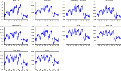
Tables 1 and 2 also present the results of the Phillips and Perron (1988) test to examine the stationarity of variables. The unit root tests in Table 1 indicate that housing prices are not stationary and that they are identified with the I(1) series. Therefore, in the empirical tests, the original data of housing prices are not directly used. Table 2 shows that trading volume are stationary series. Thus, the original data of the trading volume are used in the quantile regression. Figure 1 shows the regional house price trends in the UK, and Figure. 2 presents the regional housing market transaction volume. Despite similarities in the house price and transaction volume trends for the different regions, a significant difference is indicated between their fluctuation and volatility levels. This study proceeds to explore the differences in the depth of these markets.

Figure 1. Time series of house prices.

Source: Author’s calculations based on the data from the website of the Land Registry.

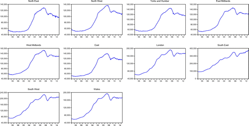
Figure 2. Time series of trading volume.

Source: Author’s calculations based on the data from the website of the Land Registry.

To estimate the fundamental level of the housing price, three macroeconomics variables are considered: interest rate, CPI, and unemployment rate. The sample time period and the data frequency for the macroeconomic variables coincided with the housing price and the volume data series. The data on the macroeconomic variables during the time interval are obtained from the Datastream database. The historical time series of the three macroeconomic variables are shown in Figure 3. As shown in Figure 3, macroeconomic performance markedly changes after 2008. The unemployment rate abruptly increases in 2008, thus decreasing housing demand. In adopting a monetary-easing environment, the UK central bank decreased the interest rate to address recession. Such reduction induced an increase in housing demand. In the data period, the CPI continued to increase. Given that housing is usually regarded as an asset that could hedge the inflation risk, the increased CPI may further increase the housing price.

Figure 3. Time series of macroeconomics variables.

Source: Author’s calculations based on the data from the Datastream database.

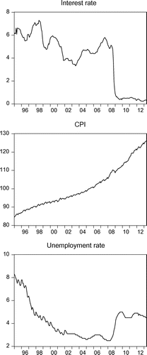
Table 3 shows the simple statistics and the results of the unit root tests of the three macroeconomic variables used in this study. The unit root tests in Table 3 indicate that the three macroeconomic variables are identified as I(1) series. Given that housing prices are also I(1) series, cointegration tests can be used to obtain the long-term equilibrium of housing prices.

Table 3. Descriptive statistics of macroeconomic variables.

	r (%)	CPI (index)	U (%)
Mean	4.0127	101.0054	4.1710
Std. Dev.	2.2159	11.2112	1.4568
Skewness	−0.6624	0.6802	1.0856
Kurtosis	2.0615	2.3515	3.5541
Unit Root test
PP test (Level)	−0.7469 (0.83)	4.1418 (1.00)	−2.2365 (0.47)
PP test (Differenced)	−8.3273 (0.00)	−15.6214 (0.00)	−9.3138 (0.00)

Notes: r, CPI, and U denote the interest rate, consumer price index and unemployment rate, respectively. PP tests are adopted for testing the null hypothesis of a unit root in the series. Intercept is included in the testing equation and lag length of the unit root models are selected by Schwarz Information Criterion. Entries in parenthesis stands for the p-value.

Source: Author’s calculations based on the data from the Datastream database.

4.2. Empirical results

The responsiveness of housing prices to changes in volume is first analysed to observe the depth of the housing markets. The results using the individual series are shown in Table 4. Only two regions, North East and North West, exhibit significant responsiveness. The average of the trading volume is also relatively low in North East, indicating lower liquidity in the regional market. The two regional housing markets are thinner than other markets. Thus, trading activity in these two markets can significantly influence the performance of housing prices. However, in the other regional markets, housing price exhibits no significant response to changes in trading behaviours. These results can be attributed to the problems of serial correlation and endogeneity of the variables. The study thus proceeds with the estimation using panel data.

Table 4. The responsiveness of housing prices to changes in volume: Individual data.

	NE	NW	Y&H	EM	WM	E	L	SE	SW	W
α	−0.0045	−0.0080	−0.0012	−0.0052	−0.0069	−0.0007	−0.0002	0.0027	0.0013	0.0057
	(0.0126)	(0.0118)	(0.0122)	(0.0130)	(0.0125)	(0.0131)	(0.0124)	(0.0106)	(0.0124)	(0.0126)
β	1.8312	2.5669	0.4351	1.5434	1.9701	0.4374	0.1190	−0.4225	−0.2512	−1.0869
	(0.8163)	(0.9908)	(0.9703)	(1.1439)	(1.1852)	(0.9450)	(1.1802)	(0.8846)	(1.2096)	(1.1203)
Loglikelihood	61.6619	79.1925	72.0840	63.6786	74.1831	57.7544	85.5197	132.2068	90.9945	80.2588

Notes: NE, NW, Y&H, EM, WM, E, L, SE, SW, W are the estimated results using the data from North East, North West, Yorks and Humber, East Midlands, West Midlands, East, London, South East, South West, Wales regions, respectively. Entries in parenthesis stands for Standard Error. The number in bold denotes significance at the 5%.

The equation for estimating the responsiveness of housing prices ($\frac{\Delta HP}{\mathit{HP}}$) to changes in volume ($\frac{\Delta Volume}{\mathit{Volume}}$) is: ${\left(\frac{\mathrm{\Delta }Volume}{\mathit{Volume}}\right)}_{i,t}=\alpha +\beta \left({\frac{\mathrm{\Delta }HP}{\mathit{HP}}}_{i,t}+{\epsilon }_{i,t}\right)$

Source: Author’s calculations based on the data from the website of the Land Registry.

The estimation using the panel data is shown in Table 5. The North East, North West, and Welsh markets show significant responsiveness. In these markets, the housing prices are significantly related to the changes in trading volume. Table 5 also presents the ‘group’ result, which indicates the significantly positive relationships between the changes in housing prices and the trading volume. On the average, the change in volume by 1.42% is estimated to change housing prices by 1%.

Table 5. The responsiveness of housing prices to changes in volume: Panel data.

Region	Coefficient	t-Statistic
(1) North East	1.2198	2.104
(2) North West	1.751	2.3225
(3) Yorkshire and The Humber	0.4355	0.6223
(4) East Midlands	0.8795	1.0655
(5) West Midlands	1.3561	1.5465
(6) East	0.3219	0.4905
(7) London	0.3672	0.3813
(8) South East	0.3135	0.3671
(9) South West	0.2549	0.2417
(10) Wales	7.3203	2.4172
Group	1.422	3.6511

Source: Author’s calculations based on the data from the website of the Land Registry.

This study proceeds with the next method, which is to estimate the depth of these housing markets. Directly assessing the liquidity parameter proposed by Kyle (1985), the long-run equilibrium level (fundamental value) of housing price is first estimated. The long-term relationships between the 10 regional housing prices and the three macroeconomic variables are examined by traditional cointegration tests (Johansen, 1988).

Table 6 presents the results of Johansen’s cointegration analysis. Based on trace statistics and the maximum eigenvalue statistics, the null hypothesis of no cointegration is rejected. Cointegration tests indicate a cointegration vector (long-term equilibrium relation) in these variables. A common stochastic trend is indicated, suggesting a stable long-term equilibrium relationship between the housing prices and these macroeconomic variables. Therefore, the three major macroeconomic variables are used to determine the equilibrium level of price. The error terms of the cointegration vector (long-run equilibrium relation) obtained from Table 6 represent the housing price deviations from the fundamental level. In addition, all error terms represent the housing price deviations regardless of whether housing price is higher or lower than the fundamental level. Therefore, in the current study, the absolute values of the error terms are used as the proxy variables of housing price deviations. This study further demonstrates the relations between the estimated deviations of the housing prices and the trading volume in the 10 regional housing markets. The results are shown in Table 7.

Table 6. Cointegration tests of housing price and macroeconomics variables.

	NE	NW	Y&H	EM	WM	E	L	SE	SW	W
Trace	63.2033	63.3178	62.7268	68.8170	70.3523	64.3587	63.5288	61.2164	63.1448	63.5192
Statistic	(0.0010)	(0.0009)	(0.0011)	(0.0002)	(0.0001)	(0.0007)	(0.0009)	(0.0017)	(0.0010)	(0.0009)
Max-Eigen	29.6237	30.1148	28.7097	27.8658	27.6442	28.2941	26.3756	25.7783	27.3132	29.3332
Statistic	(0.0270)	(0.0231)	(0.0358)	(0.0460)	(0.0491)	(0.0405)	(0.0708)	(0.0836)	(0.0541)	(0.0295)

Notes: NE, NW, Y&H, EM, WM, E, L, SE, SW, W are the estimated results using the data from North East, North West, Yorks and Humber, East Midlands, West Midlands, East, London, South East, South West, Wales regions, respectively. Intercept is included in the testing equation. Entries in parenthesis stands for the p-value. The null hypothesis of cointegration test is there is no cointegration relation existed.

Source: Author’s calculations based on the data from the Datastream database.

Table 7. The estimated liquidity parameter ($\lambda$) using OLS estimation.

	NE	NW	Y&H	EM	WM	E	L	SE	SW	W
Coefficient	3.1348	1.0858	1.5769	1.6787	1.5574	2.9987	1.3098	1.4141	0.8929	1.5231
Std. Error	0.1522	0.0535	0.0741	0.0733	0.0695	0.1429	0.0563	0.0724	0.0396	0.0673
t-Statistic	20.5931	20.3040	21.2780	22.8908	22.4110	20.9841	23.2466	19.5242	22.5252	22.6467
p-value	0.00	0.00	0.00	0.00	0.00	0.00	0.00	0.00	0.00	0.00

Notes: NE, NW, Y&H, EM, WM, E, L, SE, SW, W are the estimated results using the data from North East, North West, Yorks and Humber, East Midlands, West Midlands, East, London, South East, South West, Wales regions, respectively.

The equation for estimating the liquidity parameter is: $H{P}_t-H{P}_t^{\ast }=\lambda Volum{e}_t$ where HP is housing price, HP* is the fundamental value of housing price, Volume is trading volume. $\lambda$ represents the relationship between deviations of housing price and trading volume, which is a liquidity parameter.

Source: Author’s calculations based on the data from the website of the Land Registry.

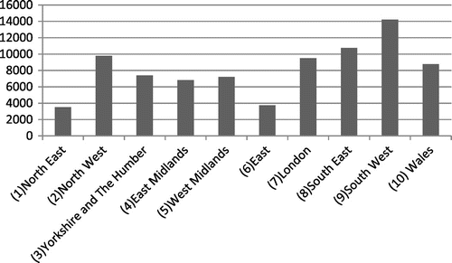
The deviations and the volume exhibit significant relations. This finding indicates that the liquidity parameters ($\lambda$) proposed by Kyle (1985) in the 10 regional housing markets are significantly positive. The significant parameters represent the trading volume (trading activity) that would cause a variation in the housing price. To illustrate the estimated depth ($\frac{1}{\lambda }$) of the 10 regional housing markets, the different market depths in the 10 regional housing markets are presented in Figure 4. The market depth in the North-East region is determined as the thinnest. Given that trading volume is also an indicator of liquidity, the averages of the trading volumes in the 10 regional housing markets are presented in Figure 5 for comparison. The results in Figure 4 are consistent with those in Figure 5. That is, the estimated market depth is positively related to trading volume.

Figure 4. Estimated market depth.

Source: Author’s calculations based on the data from the website of the Land Registry.

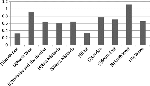
Figure 5. Average volume.

Source: Author’s calculations based on the data from the website of the Land Registry.

This study further estimates the quantile regression models to describe the relationships between the housing price deviations from the fundamental level and the trading volume, hence, the calculation of the liquidity parameter $\lambda$ proposed by Kyle (1985). This article uses the quantile regression model to estimate $\lambda$ for different conditional quantile functions. This method is adopted to comprehensively analyse the market depth under different housing price deviations. The results of quantile regression models are shown in Table 8.

Table 8. Quantile regression.

	Quantile	$\lambda$	Std. Error	t-Statistic	p-value
North	0.1	0.6357	0.1408	4.5152	0.0000
East	0.2	1.0904	0.1682	6.4834	0.0000
	0.3	1.6484	0.2072	7.9558	0.0000
	0.4	2.3986	0.2672	8.9777	0.0000
	0.5	3.1728	0.2804	11.3171	0.0000
	0.6	4.0894	0.2388	17.1223	0.0000
	0.7	4.6722	0.2315	20.1786	0.0000
	0.8	5.2134	0.2217	23.5168	0.0000
	0.9	6.0707	0.2693	22.5454	0.0000
North	0.1	0.1747	0.0525	3.3279	0.0010
West	0.2	0.3615	0.0582	6.2111	0.0000
	0.3	0.5968	0.0713	8.3688	0.0000
	0.4	0.8244	0.0882	9.3473	0.0000
	0.5	1.0758	0.0988	10.8913	0.0000
	0.6	1.3847	0.0849	16.3109	0.0000
	0.7	1.6261	0.0813	20.0026	0.0000
	0.8	1.8008	0.0814	22.1205	0.0000
	0.9	2.1546	0.1123	19.1813	0.0000
Yorkshire	0.1	0.2871	0.0737	3.8954	0.0001
and	0.2	0.5735	0.0846	6.7761	0.0000
The	0.3	0.8662	0.1053	8.2263	0.0000
Humber	0.4	1.2372	0.1325	9.3343	0.0000
	0.5	1.6111	0.1324	12.1719	0.0000
	0.6	1.9898	0.1125	17.6830	0.0000
	0.7	2.2840	0.1080	21.1465	0.0000
	0.8	2.5811	0.1118	23.0891	0.0000
	0.9	3.0478	0.1496	20.3793	0.0000
East	0.1	0.4007	0.0786	5.0970	0.0000
Midlands	0.2	0.6975	0.0869	8.0245	0.0000
	0.3	0.9705	0.0972	9.9800	0.0000
	0.4	1.2729	0.1179	10.7954	0.0000
	0.5	1.6184	0.1313	12.3254	0.0000
	0.6	1.9620	0.1201	16.3346	0.0000
	0.7	2.3946	0.1162	20.6067	0.0000
	0.8	2.6511	0.1126	23.5520	0.0000
	0.9	3.1673	0.1504	21.0563	0.0000
West	0.1	0.3505	0.0716	4.8927	0.0000
Midlands	0.2	0.5955	0.0806	7.3905	0.0000
	0.3	0.8538	0.0930	9.1761	0.0000
	0.4	1.1830	0.1160	10.1965	0.0000
	0.5	1.5199	0.1310	11.6016	0.0000
	0.6	1.9549	0.1097	17.8218	0.0000
	0.7	2.2061	0.1017	21.6946	0.0000
	0.8	2.5086	0.1060	23.6627	0.0000
	0.9	2.9222	0.1323	22.0959	0.0000
East	0.1	0.6113	0.1353	4.5187	0.0000
	0.2	1.1065	0.1587	6.9708	0.0000
	0.3	1.5620	0.1852	8.4333	0.0000
	0.4	2.2674	0.2364	9.5920	0.0000
	0.5	2.8689	0.2713	10.5750	0.0000
	0.6	3.8235	0.2338	16.3511	0.0000
	0.7	4.3587	0.2179	20.0065	0.0000
	0.8	5.1287	0.2366	21.6753	0.0000
	0.9	5.8922	0.2820	20.8963	0.0000
London	0.1	0.3221	0.0645	4.9946	0.0000
	0.2	0.5690	0.0682	8.3459	0.0000
	0.3	0.7877	0.0774	10.1816	0.0000
	0.4	1.0429	0.0818	12.7438	0.0000
	0.5	1.2806	0.0818	15.6533	0.0000
	0.6	1.4644	0.0794	18.4357	0.0000
	0.7	1.7182	0.0838	20.5030	0.0000
	0.8	2.0130	0.1017	19.8013	0.0000
	0.9	2.5422	0.1505	16.8928	0.0000
South	0.1	0.2124	0.0799	2.6593	0.0084
East	0.2	0.5304	0.0765	6.9343	0.0000
	0.3	0.8080	0.0826	9.7875	0.0000
	0.4	0.9858	0.0885	11.1374	0.0000
	0.5	1.3107	0.0969	13.5254	0.0000
	0.6	1.5619	0.1117	13.9881	0.0000
	0.7	1.9058	0.1168	16.3104	0.0000
	0.8	2.3694	0.1433	16.5348	0.0000
	0.9	2.9606	0.1974	14.9958	0.0000
South	0.1	0.2213	0.0430	5.1510	0.0000
West	0.2	0.3660	0.0489	7.4897	0.0000
	0.3	0.5379	0.0543	9.9030	0.0000
	0.4	0.6998	0.0546	12.8119	0.0000
	0.5	0.8696	0.0531	16.3672	0.0000
	0.6	1.0034	0.0529	18.9560	0.0000
	0.7	1.1385	0.0574	19.8433	0.0000
	0.8	1.3694	0.0723	18.9366	0.0000
	0.9	1.7803	0.1149	15.4981	0.0000
Wales	0.1	0.3097	0.0819	3.7818	0.0002
	0.2	0.6602	0.0811	8.1439	0.0000
	0.3	0.8856	0.0908	9.7573	0.0000
	0.4	1.1880	0.0990	12.0000	0.0000
	0.5	1.5166	0.1037	14.6214	0.0000
	0.6	1.7297	0.1003	17.2392	0.0000
	0.7	2.0619	0.1028	20.0531	0.0000
	0.8	2.3979	0.1148	20.8913	0.0000
	0.9	2.9839	0.1772	16.8399	0.0000

Source: Author’s calculations based on the data from the website of the Land Registry.

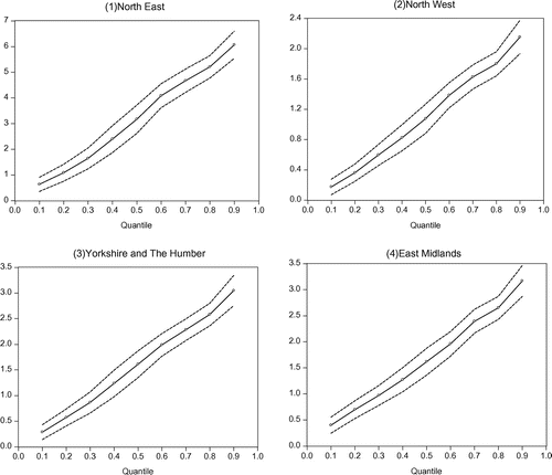
Table 8 shows that coefficients ($\lambda$) obtained from different quantile functions markedly vary. Thus, the depth of the housing market ($\frac{1}{\lambda }$) is significantly related to the housing price deviations from the fundamental level. The coefficients tend to become large and significant when the deviations are high. Figure 6 presents the coefficients showing the relation between the deviations and the volumes under different quantile regressions. The area between the dotted lines indicates its corresponding 95% confidence interval. These data can provide in-depth understanding of the relationship, especially when the conditional distribution is heterogeneous. The 10 regions exhibit a similar pattern in the various coefficients obtained by different quantile functions. The liquidity parameter $\lambda$ is positively related to the housing price deviations, suggesting a negative relation between the depth of the housing market ($\frac{1}{\lambda }$) and the housing price deviation. Table 8 and Figure 6 indicate that a thinner housing market tends to exhibit more housing price deviations attributed to temporary changes in volume.

Figure 6. The estimation of $\lambda$.

Source: Author’s calculations based on the data from the website of the Land Registry.

As shown in Table 9, a robustness test is conducted. Price change is substituted for the housing price deviations from the fundamental level to estimate (6). The substitution enables verifying the necessity of conducting an estimation by using the deviations in Table 7. The results in Table 9 indicate that in Table 7, the neighbourhoods with estimated high values of liquidity parameters (λ) such as the North East and East, display proportionally high values in Table 9. In other words, both the volume–price deviations and the volume–price change methods yield identical results for comparing local market depths. However, employing only the price change caused by transaction volume to explain the market depth is not as rigorous as the methods employed by studies regarding other markets.

Table 9. The estimated liquidity parameter ($\lambda$) using changes of housing price.

	NE	NW	Y&H	EM	WM	E	L	SE	SW	W
Coefficient	0.1032	0.0404	0.0553	0.0641	0.0620	0.1128	0.0693	0.1361	0.0552	0.0738
Std. Error	0.0245	0.0070	0.0105	0.0102	0.0092	0.0223	0.0084	0.0159	0.0065	0.0101
t-Statistic	4.2213	5.7939	5.2772	6.2773	6.7450	5.0544	8.2468	8.5549	8.5445	7.3092
p-value	0.00	0.00	0.00	0.00	0.00	0.00	0.00	0.00	0.00	0.00

Notes: NE, NW, Y&H, EM, WM, E, L, SE, SW, W are the estimated results using the data from North East, North West, Yorks and Humber, East Midlands, West Midlands, East, London, South East, South West, Wales regions, respectively.

The equation for estimating the liquidity parameter is: $H{P}_t-H{P}_{t-1}=\lambda Volum{e}_t$ where HP is housing price, Volume is trading volume. $\lambda$ represents the relationship between changes of housing price and trading volume, which is a liquidity parameter.

Source: Author’s calculations based on the data from the website of the Land Registry.

5. Conclusion

This study focuses on the price–volume correlations in the UK housing markets to analyse market depth. Adopting the concept of market depth proposed by Kyle (1985), this study employs regional data from the UK housing market to analyse the trading volume required to move prices by one unit. The relationships between house prices and trading volumes are not significant, as indicated by the results in the individual series. However, the results obtained using the panel data show that an average change in volume by 1.42% would cause a change in the housing price by 1%.

This study directly estimates the liquidity parameter, which represents the relationship between the housing price deviations from the fundamentals and the trading volume. By OLS estimation, the depth of market is shown to be consistent with the trading volume across the regional housing markets. Using quantile regression, this study shows the significant relation between the depth of housing market and the housing price deviations from the fundamental level. A thinner housing market indicates more housing price deviations caused by temporary changes in volume.

This study illustrates another indicator of liquidity and explores the responsiveness of housing price in different regional housing markets. Given that the lack of liquidity is a potential cause of inefficiency of the housing market, market depth analysis can predict the response of the housing price and evaluate the effectiveness and the effects of policies in different housing markets.

Studies on the UK housing market have mostly examined the efficiency comparisons of various regional housing markets and correlations of regional housing prices. The present study describes the regional housing market depths and verifies the relationships between the transaction volume and housing price deviations. Subsequent studies should investigate whether the market depth causes the correlation or inefficiency of the regional UK housing market.

If the UK housing policies enable market depth increase, the UK housing market will be more efficient, and short-term deviations of housing prices will occur less often. For UK citizens and investors, a high frequency of buying or selling caused by relocation needs may result in irrational price changes when regional housing market depths are low. Such a phenomenon of housing price deviations determines whether the current market favours buyers or sellers.

Disclosure statement

No potential conflict of interest was reported by the authors.

Notes

1. Wheaton (1990) found that increased volume consequently shortens the selling time and influences the price. Berkovec and Goodman (1996) indicated that the volume varies more quickly than the price. Hort (2000) studied the housing market in Sweden and found that under asymmetric property market information volume affects price because the demand adjustment caused by the housing price fluctuation is extremely slow. The empirical results in Leung et al. (2002) based on the data reflecting the housing market in Hong Kong showed that volume affects price in many individual cases. Clayton et al. (2010) used the volume as a proxy variable of liquidity and found that quarterly price–volume correlation is not significant. However, the annual data, reveal that the volume controls the price.

2. Zhou (1997) analysed the American housing market and applied cointegration and causality tests, discovering that these two variables are cointegrated and that price affects volume.

3. Engle and Lange (2001) illustrated the hypothetical expected transaction price for various size buying or selling orders. They proposed that this schedule is often called the market reaction curve.

References

- Admati, A. R., & Pfleiderer, P. (1988). A Theory of Intraday Patterns: Volume and Price Variability. Review of Financial Studies, 1(1), 3–40.10.1093/rfs/1.1.3
- Ahn, H. J., Bae, K. H., & Chan, K. (2001). Limit orders, depth, and volatility: Evidence from the stock exchange of Hong Kong. The Journal of Finance, 56(2), 767–788.10.1111/0022-1082.00345
- Aoki, K., Proudman, J., & Vlieghe, G. (2002). Houses as collateral: Has the link between house prices and consumption in the UK changed? Federal Reserve Bank of New York Economic Policy Review, 8(1), 163–177.
- Berkovec, J. A., & Goodman, J. L. (1996). Turnover as a measure of demand for existing homes. Real Estate Economics, 24(4), 421–440.10.1111/reec.1996.24.issue-4
- Bessembinder, H., & Seguin, P. J. (1993). Price volatility, trading volume, and market depth: Evidence from futures markets. The Journal of Financial and Quantitative Analysis, 28(1), 21–39.10.2307/2331149
- Biais, B., & Weill, P-O. (2009). Liquidity shocks and order book dynamics ( TSE working paper NO. 09-037). Toulouse School of Economics. Retrieved from http://www.tse-fr.eu/sites/default/files/medias/doc/wp/fit/wp_fit_37_2009.pdf 10.3386/w15009
- Brooks, R., Harris, E., & Joymungul, Y. (2009). Market depth in an illiquid market: Applying the VNET concept to Victorian water markets. Applied Economics Letters, 16(13), 1361–1364.10.1080/13504850701426571
- Case, K. E., & Shiller, R. J. (1989). The efficiency of the market for single-family homes. American Economic Review, 79(1), 125–137.
- Chen, N., Kou, S., & Wang, C. (2015). A partitioning algorithm for Markov decision processes and its applications to market microstructure ( Working paper). doi:10.2139/ssrn.2360552
- Clayton, J. (1998). Further evidence on real estate market efficiency. Journal of Real Estate Research, 15(1), 41–57.
- Clayton, J., Miller, N., & Peng, L. (2010). Price-volume correlation in the housing market: Causality and co-movements. The Journal of Real Estate Finance and Economics, 40(1), 14–40.10.1007/s11146-008-9128-0
- Elbourne, A. (2008). The UK housing market and the monetary policy transmission mechanism: An SVAR approach. Journal of Housing Economics, 17(1), 65–87.10.1016/j.jhe.2007.09.002
- Engle, R. F., & Lange, J. (2001). Predicting VNET: A model of the dynamics of market depth. Journal of Financial Markets, 4(2), 113–142.10.1016/S1386-4181(00)00019-7
- Fung, H. G., & Patterson, G. A. (1999). The dynamic relationship of volatility, volume, and market depth in currency futures markets. Journal of International Financial Markets, Institutions and Money, 9(1), 33–59.10.1016/S1042-4431(98)00035-3
- Gathergood, J. (2011). Unemployment risk, house price risk and the transition into home ownership in the United Kingdom. Journal of Housing Economics, 20(3), 200–209.10.1016/j.jhe.2011.03.001
- Gau, G. W. (1985). Public Information and abnormal returns in real estate investment. Real Estate Economics, 13(1), 15–31.10.1111/reec.1985.13.issue-1
- Goettler, R. L., Parlour, C. A., & Rajan, U. (2009). Informed traders and limit order markets. Journal of Financial Economics, 93(1), 67–87.10.1016/j.jfineco.2008.08.002
- Goldstein, M. A., & Kavajecz, K. A. (2000). Eighths, sixteenths, and market depth: Changes in tick size and liquidity provision on the NYSE. Journal of Financial Economics, 56(1), 125–149.10.1016/S0304-405X(99)00061-6
- Gu, A. Y. (2002). The predictability of house prices. Journal of Real Estate Research, 24(3), 213–234.
- Hort, K. (2000). Prices and turnover in the market for owner-occupied homes. Regional Science and Urban Economics, 30(1), 99–119.10.1016/S0166-0462(99)00028-9
- Iacoviello, M. (2005). House prices, borrowing constraints, and monetary policy in the business cycle. American Economic Review, 95(3), 739–764.10.1257/0002828054201477
- Johansen, S. (1988). Statistical analysis of cointegration vectors. Journal of Economic Dynamics and Control, 12(2–3), 231–254.
- Kavajecz, K. A. (1999). A specialist’s quoted depth and the limit order book. The Journal of Finance, 54(2), 747–771.10.1111/0022-1082.00124
- Kempf, A., & Korn, O. (1999). Market depth and order size. Journal of Financial Markets, 2(1), 29–48.10.1016/S1386-4181(98)00007-X
- Koenker, R., & Bassett, G., Jr (1978). Regression quantiles. Econometrica, 46(1), 33–50.10.2307/1913643
- Koenker, R. W., & d’Orey, V. (1987). Algorithm AS 229: Computing regression quantiles. Journal of the Royal Statistical Society. Series C (Applied Statistics), 36(3), 383–393.
- Kyle, A. S. (1985). Continuous auctions and insider trading. Econometrica, 53(6), 1315–1336.10.2307/1913210
- Lee, C. M., Mucklow, B., & Ready, M. J. (1993). Spreads, depths, and the impact of earnings information: An intraday analysis. Review of Financial Studies, 6(2), 345–374.10.1093/rfs/6.2.345
- Leung, C., Lau, G., & Leong, Y. (2002). Testing alternative theories of the property price-trading volume correlation. Journal of Real Estate Research, 23(3), 253–263.
- Mikhed, V., & Zemčík, P. (2009). Do house prices reflect fundamentals? Aggregate and panel data evidence. Journal of Housing Economics, 18(2), 140–149.10.1016/j.jhe.2009.03.001
- Mishkin, F. S. (2007). Housing and monetary transmission mechanism ( NBER working papers 13518). National Bureau of Economic Research. Retrieved from http://www.nber.org/papers/w13518 10.3386/w13518
- Muellbauer, J., & Murphy, A. (2008). Housing markets and the economy: The assessment. Oxford Review of Economic Policy, 24(1), 1–33.10.1093/oxrep/grn011
- Pedroni, P. (2001). Fully modified OLS for heterogeneous cointegrated panels. Advances in Econometrics, 15, 93–130.
- Phang, S. Y. (2004). House prices and aggregate consumption: Do they move together? Evidence from Singapore. Journal of Housing Economics, 13(2), 101–119.10.1016/j.jhe.2004.04.003
- Phillips, P. C., & Moon, H. R. (1999). Linear regression limit theory for nonstationary panel data. Econometrica, 67(5), 1057–1111.10.1111/ecta.1999.67.issue-5
- Phillips, P. C., & Perron, P. (1988). Testing for a unit root in time series regression. Biometrika, 75(2), 335–346.10.1093/biomet/75.2.335
- Pradhan, R. P., Arvin, M. B., & Ghoshray, A. (2015). The dynamics of economic growth, oil prices, stock market depth, and other macroeconomic variables: Evidence from the G-20 countries. International Review of Financial Analysis, 39, 84–95.10.1016/j.irfa.2015.03.006
- Ranaldo, A. (2004). Order aggressiveness in limit order book markets. Journal of Financial Markets, 7(1), 53–74.10.1016/S1386-4181(02)00069-1
- Tsai, I.-C. (2014). Ripple effect in house prices and trading volume in the UK housing market: New viewpoint and evidence. Economic Modelling, 40, 68–75.10.1016/j.econmod.2014.03.026
- Tsai, I.-C. (2015). Information content in the depth of futures markets. Investment Analysts Journal, 44(1), 43–56.
- Vargas-Silva, C. (2008). Monetary policy and the US housing market: A VAR analysis imposing sign restrictions. Journal of Macroeconomics, 30(3), 977–990.10.1016/j.jmacro.2007.07.004
- Wheaton, W. C. (1990). Vacancy, search, and prices in a housing market matching model. Journal of Political Economy, 98(6), 1270–1292.10.1086/261734
- Zhou, Z. G. (1997). Forecasting sales and price for existing single-family homes: A VAR model with error correction. Journal of Real Estate Research, 14(2), 155–167.