Is there any relationship between producer price index and consumer price index in the Czech Republic?

Abstract

This article tests the expenditure-switching model in the Czech Republic to inspect the causal link between the Producer Price Index (P.P.I.) and Consumer Price Index (C.P.I.). The results of the co-movement between the P.P.I. and C.P.I. in the period indicate a positive relationship across the chosen period. We notice that in the frequency domain, the two variables have a relationship in higher spectrums (short-term). The results also show that co-movements exist during structural reforms and financial crises, which in turn supports the expenditure-switching model. The C.P.I. and P.P.I. are sensitive to variations in exchange rates, which pass through prices at the domestic level. Exchange rate shocks lead to inflationary pressure; therefore, long-term oriented intervention policies of the central banks will be more efficient. This article provides substantial information to exporters about price adjustments to exchange rate fluctuation.

Keywords:

• Producer price index (P.P.I.)
• Consumer price index (C.P.I.)
• exchange rate
• wavelet analysis

JEL classification:

• E31
• F31

1. Introduction

Price stability is one of the major macroeconomic objectives of an economy (Lado, 2015). It promotes employment and economic growth, reduces the risk premium and promotes financial stability (Szymańska, 2011). Conversely, inflation weakens currency performance in an economy, affecting the primary currency functions of storing value and providing a reliable medium of exchange (Mandizha, 2014). Rising inflation challenges economic growth by reducing purchasing power, the value of investments and saving. In general, inflation constitutes a cost for households and businesses (Daniela, Mihail-Ioan, & Sorina, 2014). It reduces welfare and generates uncertainty in output (Ball, 1992; Friedman, 1977). The exchange rate is considered an essential component in inflation forecasting and has attracted close attention from investors, banks and policy makers (Lyócsa, Molnár, & Fedorko, 2016). The inflow of capital due to the liberalisation process has emphasised the importance of stabilising the exchange rate (Geršl & Holub, 2006). Domestic prices are sensitive because of the effect of the exchange rate on import prices (Calvo & Reinhart, 2000). Thus, an appropriate monetary policy and price stability are necessary. Imported intermediate and domestically produced goods are the connecting link between the exchange rate and both price indices (An & Wang, 2012). The exchange rate is indispensable for both the policymaker and market participants to collect information for monetary policy execution; it helps the central bank to develop fixed policy instruments (Adámek, 2016). The exchange rate is important for small economies, serving as a macroeconomic indicator, and is perceived as a connection between the financial and the real economy (Nalban, 2015; Triandafil, Brezeanu, Huidumac, & Triandafil, 2011). Several studies show that the exchange rate might have a greater bearing on the Producer Price Index (P.P.I.) than on the Consumer Price Index (C.P.I.) (Martinez, Caicedo, & Tique, 2013). A devalued currency increases import prices and places pressure on inflation, whereas appreciation helps inflation to decrease.

The sensitivity of price indices to shocks in exchange rates is critical in the case of small open economies such as the Czech Republic (Geršl & Houlb, 2006), which began its independent economic and monetary existence as early as 1993. The country attracts massive foreign capital inflow due to the stable exchange rates, high interest rates and greater political stability (Kurihara, 2012). The idea of inflation targeting was initiated by the Czech Bank (C.R.B.) in 1998 because of the financial crisis in 1997 and numerous macroeconomic hazards such as high inflation and interest rates, exchange rate depreciation and a current account deficit (Hájek & Horváth, 2015). To address inflation, the Czech Republic was the first country of the former European communist block to initiate inflation targeting strategies (Holub & Huník, 2008). However, economic growth started to decline due to weak exports, high imports and the currency crisis in Asia. The country introduced a flexible exchange rate in May 1997 after some exchange rate turbulence. The Czech economy went through a period of reemergence from 1998 to 2000 characterised by relative currency stability and low inflation (Beblavý, 2007).

In 2002, a massive capital inflow and appreciation of the Czech Koruna (C.Z.K.) resulted in increases in the C.P.I. and P.P.I. However, in 2007, the depreciation largely resulted from the “carry trade”¹ operation, in which investors were attracted to buy Czech assets due to the uncertainty that prevailed in the global markets. From 2007 to 2008, the C.P.I. witnessed its greatest increase because of administrative prices and high global energy prices. Economic growth continued after the E.U. accession and was less affected by the financial crisis in 2008. However, the industrial production of the Czech Republic dropped at a two-digit rate due to its linkage to Germany and other countries affected by the financial crisis. Both the P.P.I. and C.P.I. recorded decreases due to the decrease in demand for Czech products and the fall of commodity prices at the global level. The economy recovered at the start of 2010, and price indices saw a slightly increasing trend during this time. The Czech Republic once again fell into a recession in 2012 due to a reduction in external demand and to government austerity measures. The C.P.I. decreased in 2013, largely being driven by administrative costs such as indirect taxes. In November 2013, the C.R.B. devalued the C.Z.K. to boost exports and employment, but this measure resulted in rising inflation. The deliberate depreciation aimed to increase external demand and the price of domestic goods. After the dismal performance in 2012–2013, the Czech economy resumed growth in 2014. The weakening of the exchange rate was useful for the Czech economy, which grew by 2% in 2014. From 2013 to 2015, the P.P.I. fell by 2%, and the C.P.I. reached its lowest level, the main causes being drops in the oil, food and administered prices. The C.P.I. and P.P.I. declined due to continuing falling energy prices, and the exchange rate remained weak.

The Czech Republic is always cautious about a significant fluctuation in the exchange rate, which can hinder the export-led growth strategy and be a challenging factor for inflation (Kurihara, 2012). The economic and financial integration of the Czech Republic with other Central and Eastern European countries makes the country more vulnerable to external shocks emanating from its trading partners (Baghestani & Danila, 2014); currency appreciation in 2002–2008 decreased the price competitiveness of the domestic economy and led to falling inflation rates. However, depreciation had the reverse effect on inflation in 2000–2002, when the Czech Republic recorded high inflation. The exchange rate had a significant role in the C.P.I. and P.P.I. over the years, particularly in the financial crisis in 2008 and in the eurozone debt crisis.

The inflation targeting, the global financial crisis and deliberate devaluation of the exchange rate caused structural changes that caused the C.P.I. and P.P.I. nexus to be unstable in the Czech Republic. This study explores the presence of structural changes, implying that the relationship between the P.P.I. and C.P.I. is complicated and varies over time. The finding supports the expenditure-switching model, which states a significant aspect of the exchange rate in both the P.P.I. and C.P.I. The study can contribute to the inflation targeting policy by giving attention to the C.P.I. and the prediction of the P.P.I. in the production stage.

This article is organised as follows: Section 2 consists of the literature review. Section 3 provides the theoretical model base. Section 4 describes the methodology. Section 5 analyses the data and explains the results. Section 6 concludes.

2. Literature review

Several studies elaborate the links among the exchange rate, P.P.I. and C.P.I. McCarthy (1999) estimates the exchange rate contribution to the domestic P.P.I. and C.P.I. in six O.E.C.D. countries by employing the recursive framework method. The result indicates that the exchange rate has a modest influence on local prices. Bhattacharya and Thomakos (2008) consider the effect of the exchange rate on the P.P.I. and C.P.I. and confirm that accurate forecasting is possible when the exchange rate pass effect is included. Ito and Sato (2007) indicate that the exchange rate played an important part in the C.P.I. in the Latin countries. Ocran (2010) indicates that a 1% change in the exchange rate causes an increase of 0.125% and 20% in the C.P.I. and P.P.I., respectively. Adetiloye (2010) indicates that the exchange rate has a small but meaningful effect on C.P.I. Imimole and Enoma (2011) find that exchange rate depreciation has a long-term positive effect on the C.P.I. Jin (2012) indicates that the exchange rate plays an important part in the P.P.I. compared with C.P.I. in the long-term. An and Wang (2012) explore that the exchange rate has a higher effect on the P.P.I. compared than on the C.P.I. The result also shows that the exchange rate has a more-significant involvement in a small-size economy with a greater import share and volatile monetary policy. Zhu (2012) investigates the C.P.I. relationship with the exchange rate and shows that the exchange rate leads the C.P.I. Tiwari (2012) finds that C.P.I. leads the P.P.I. at an intermediate level of frequency. Tiwari, Suresh, Arouri, and Teulon (2014) determine a bi-directional causality between the P.P.I. and C.P.I. by using wavelet analysis. Tiwari, Mutascu and Andries (2013) use the frequency domain to evaluate the time-frequency relationship between the C.P.I. and P.P.I. and identify a cyclical effect.

Adeyemi and Samuel (2013), Uddin, Quaosar, and Nandi (2014) and Dube (2016) analyse the position of the exchange rate in the development of C.P.I. and find that the exchange rate is a significant element in explaining the C.P.I. Mohammed, Bendob, Djediden, and Mebsout (2015) conclude that appreciation of the exchange rate causes an increase in the C.P.I. but a negligible response from the P.P.I. Su, Khan, Lobont, and Sung (2016) find a short-term link between the C.P.I. and the exchange rate in China. Su, Khan, et al. (2016) and Khan, Chi-Wei, Moldovan, and Xiong (2017) explore bidirectional causality between the P.P.I. and C.P.I. and conclude that the P.P.I. has a greater contributing role to the C.P.I.

Babecká-Kucharýuková (2009) investigates the exchange rate effect on domestic inflation in the Czech Republic and finds that exchange rate shock passes through to inflation. Josifidis, Allegret, and Pucar (2009) elaborates the exchange rate implications on C.P.I. in the Czech Republic, and the outcome displays that the exchange rate explains 66% of the variation in the C.P.I., particularly in the depreciation period. Shahbaz et al. (2012) find unidirectional causality from the C.P.I. to P.P.I. at lower, medium and higher frequencies by using wavelet analysis. Nalban (2015) estimates the change in the exchange rate and subsequent implications for the C.P.I. and P.P.I. in Central Eastern European (C.E.E.) countries. It is evident that in the long-term, exchange rates influence both price indices, whereas C.P.I. only affects the short-term. Skořepa, Tomšík, and Vlcek (2016) show that in the Czech Republic, the exchange rate has a greater influence on the P.P.I. than on the C.P.I.

The above literature review indicates that these studies use the cointegration method, causality approach, autoregressive distributed lag and vector autoregression (V.A.R.). These techniques examine correlation based on a full sample and ignore sub-sample causality. Conventional methods of causality cannot identify the relationship between the full sample and sub-sample; they also lack the power to detect time variation. The examination of a lead-lag relationship at different frequencies had no application in this case (Zhou, 2010) and has the disadvantage of ignoring the time variation feature in the evaluation of the relationship between the two variables. Such methods provide no integrated basis to measure the time and frequency change characteristic. Traditional Granger causality faces the problem of model specification, a number of lags and spurious regression (non-stationarity) (Gujarati, 1995). It also lacks the characteristic of measuring Granger causality in the time domain.

This study uses wavelet analysis to explain causation between the P.P.I. and C.P.I. rate in the time and frequency domains. The method has a unique edge over traditional techniques. First, it develops the specified time series into a window to visualise both times and a changeable frequency set of information using an extremely intuitive method. Second, the wavelet analysis explores the co-movement and causality at the same time with variation over time. Third, it does not involve the constraint of a unit root test, the cointegration test, and specification of lag length. Balcilar, Ozdemir, and Arslanturk (2010) establish that relationships between the time series can create a problem of instability due to the structural changes. Thus, the results in the full sample become inappropriate for estimation.

3. Expenditure-switching model

In this study, we use the expenditure-switching model proposed by Bhattacharya and Thomakos (2008) to elucidate the relationship between the P.P.I. and C.P.I., with the exchange rate as controlling variable. The model describes the effects of the exchange rate on the consumer, producer and import prices. Alternatively, the model examines the influence of the exchange rate on the raw materials, intermediate goods and final goods. The final values are measured by the C.P.I., which is further divided into tradable and non-tradable goods. The exchange rate fluctuation would lead significant changes in prices, includes the markup price $m^{*}{}_i\ge 0$ charged by the exporter: (1) $$p_{ri}=(1+m_i{}^{*})\hspace{0.17em}E{P}^{*}$$(1) where $p_{ri}$ is the import price; E represents the exchange rate;$P^{*}$ is foreign currency price of imported goods; and $m^{*}{}_i$is the markup price. However, when the exporter has no markup, then the import price will change proportionately with the exchange rate. In the home market, retailers must pay the transportation and delivery costs of end goods, which are equal to the following: (2) $$M{C}_{ri}=P_{ri}\left(1+{\Omega }_{ri}\right)$$(2) where ${\Omega }_{ri}$ is the transaction cost of the retailer, and $M{C}_{ri}$ is the marginal cost. By adding the domestic retailer markup, the final price of goods is as follows: (3) $$P_{ci}=\left(1+{\gamma }_i\right)(1+{\Omega }_{ri})(1+m_i{}^{*}) M{C}_{ri}$$(3) where $P_{ci}$denotes the price of the final goods, and γ_i is the domestic markup of the retailer. Equation (3)(3) $$P_{ci}=\left(1+{\gamma }_i\right)(1+{\Omega }_{ri})(1+m_i{}^{*}) M{C}_{ri}$$(3) describes the final price$P_{ci}$, import price and exchange rate, with the import price increasing due to exchange rate depreciation. The variations in the foreign and domestic markup price lead the exchange rate to change in the import and domestic price. Thus, the ultimate final price of the P.P.I. can be attributed to changes in the exchange rate, locally manufactured intermediate input cost and movement in the imported raw material. The price at the entry point is equivalent to the exchange rate, foreign currency price of imported goods and the markup price: (4) $$P_{ni}=\left(1+m_{ni}{}^{*}\right){EP}^{*}$$(4) where $P_{ni}$ is the entry price, and $m^{*}{}_{ni}$ denotes the markup price of the exporter. Domestically produced goods must pay wages with the transaction cost of imported inputs. The wage is presented wage ${\omega }_i$, and $l_i$ denote the unit labor in production. The marginal cost is equal to the following: (5) $$M{C}_{ni}=P_{ni}(1+{\Omega }_{ri})+{\omega }_i{l}_i$$(5)

Assigning the domestic markup paid by the producer to ${\mu }_i$ makes the producer price as follows: (6) $$P_{pi}=\left(1+{\mu }_i\right)M{C}_{ni}$$(6)

Using Equation (6)(6) $$P_{pi}=\left(1+{\mu }_i\right)M{C}_{ni}$$(6) , we obtain: $$P_{pi}=\left(1+{\mu }_i\right)\left[{\omega }_i{l}_i+\left(1+{\Omega }_{ri}\right)\left(1+m_{ni}^{*}\right)E{P}^{*}\right]$$ where $P_{pi}$ is producer price. According to equation (6)(6) $$P_{pi}=\left(1+{\mu }_i\right)M{C}_{ni}$$(6) , P.P.I. is equal to the markup price, wages, transportation cost, markup price of the exporter and exchange rate. The above theoretical base confirms that the exchange rate is one of the factors that have an important effect on the P.P.I. and C.P.I. It influences in two forms. First, the exchange rate causes variation in import prices; second, changes in exchange rates are transmitted to the P.P.I. and the C.P.I. Therefore, we use this theoretical framework to inspect the influence of the exchange rate on the C.P.I. and P.P.I. The results indicate that the exchange rate is a major contributor in the explanation of both price indices.

4. Wavelet analysis methods

Replacing the Fourier transform technique with the wavelet approach has the advantage of including an estimation of spectral properties as a function of time (Aguiar-Conraria, Azevedo, & Soares, 2008). The wavelet approach helps to examine the affiliation between the series by considering the time and frequency domain. This approach is more appropriate and can be useful with series that are non-stationary (Roueff & Sachs, 2011). It does not require the constraint of unit root test, cointegration test, and specification of lag length.

4.1. Continuous wavelet transform

The transform is used to ascertain the character and resemblance of the data (Grinsted, Moore, & Jevrejeva, 2004; Loh, 2013)² and is applied to break down time series into wavelets. The Continuous wavelet transform (C.W.T.) is utilised to transform $x(t)$ as follows: (7) $$W_A\left(\rho ,\kappa \right)={\int }_{-\infty }^{+\infty }A\left(t\right){\beta }^{*}{}_{\rho ,\kappa }\left(t\right)dt$$(7) where ${\beta }^{*}{}_{\rho ,\kappa }$ denote the complex conjugate and can be deformed by the mother wavelet $\Psi (t)$ as ${\Psi }_{\rho ,K}(t)= \frac{1}{\sqrt{\kappa }} \Psi (\frac{t-\kappa }{\kappa })$, where κ represents the wavelet scale, and $\rho$ is theposition of the parameter that controls the center of the wavelet. By moving κ and translating along $\rho$, the amplitudes of $“C(t)”$ can be observed intuitively over scale and time (Torrence & Compo, 1998).

4.2. Wavelet power spectrum

The power spectrum is utilised to measure the localised variance of time series at all scales and frequencies, defined as ${\left|W_C(\rho ,\kappa )\right|}^2$ The modified form of the cross-wavelet transform suggested by Hudgins, Parker, and Scott (1993) can be described as follows: (8) $${\left|W_{AB}\left(\rho ,\kappa \right)\right|}^2={\left|W_A\left(\rho ,\kappa \right)\right|}^2{\left|W_B^{*}\left(\rho ,\kappa \right)\right|}^2$$(8) where * indicates the complex conjugation. The localised variance of time series $A(t)$ and $B(t)$ can be estimated using the cross-wavelet power spectrum in specified frequency domains. In this study, the wavelet power on the right hand has color lines, in which the red shades exhibit high power and the lower power is highlighted by the blue shades.

4.3. Wavelet coherency and phase difference

The cross-wavelet and auto-wavelet power spectrums are utilised to assess wavelet coherency (Torrence & Webster, 1999), defined as follows: (9) $$R_{xy}^2\left(\kappa ,\rho \right)=\frac{{\left|S\left({\kappa }^{-1}{W}_{AB}\left(\kappa ,\rho \right)\right)\right|}^2}{S\left({\kappa }^{-1}{\left|W_A\left(\kappa ,\rho \right)\right|}^2\right)S\left({\kappa }^{-1}{\left|W_B\left(\kappa ,\rho \right)\right|}^2\right)}$$(9) where $S$ is the smoothing operator obtained by modification in time and frequency (Torrence & Compo, 1998). Wavelet coherency $R_{AB}^2(\kappa ,\rho )\in \left[0,1\right]$ is calculated in a time-frequency space, and zero coherency is the proof of no correlation among the variables. The phase difference has the properties that it specifies the strength and the direction of the relationship between the variables. In other words, it provides information about which variable causes the other and whether the causality is negative or positive. The link between $A(t)$ and $B(t)$ can be described by the phase difference (Bloomfield et al., 2004) as follows: (10) $${\psi }_{AB}={\hspace{0.17em}\text{tan}\hspace{0.17em}}^{-1}\left(\frac{\mathfrak{I}\left\{S({\kappa }^{-1}{W}_{AB}(\kappa ,\rho ))\right\}}{\mathfrak{R}\left\{S({\kappa }^{-1}{W}_{AB}(\kappa ,\rho ))\right\}}\right), \text{with} {\psi }_{AB}\in \left[-\pi , \pi \right]$$(10) where $\mathfrak{I}$ and $\mathfrak{R}$ indicate the hypothetical and actual segments of the smoothed cross-wavelet transform, respectively.

The case of the zero at the phase difference indicates that both variables move together, whereas a phase difference in the form of $\pi$ ($-\pi$) indicates that the variables change oppositely. When ${\psi }_{AB}\in (0,\frac{\pi }{2})$, then $A(t)$. Granger causes a $B(t)$ with positive direction. When ${\psi }_{AB}\in (\frac{\pi }{2}, \pi )$, $B(t)$ has the predictive power of $A(t)$ with negative direction. The variable will move out of the phase if ${\psi }_{AB}\in (-\pi ,-\frac{\pi }{2})$, indicating that $A(t)$ causes $B(t)$ and is in phase if ${\psi }_{AB}\in (-\frac{\pi }{2},0)$, with $B(t)$ forecasting$A(t)$

The present study elucidates the relationship between the P.P.I. and C.P.I. in the presence of exchange rate as a controlling variable. Given the causal link between the three variables, we first inspect the causality between the P.P.I. and C.P.I. Second, the causality between the exchange rate and P and on the C.P.I. individually is estimated. In this stage, we employ partial wavelet coherency and partial phase difference. After controlling the $C(t)$, the connection between $A(t)$ and $B(t)$ is called squared partial wavelet coherency (Aguiar-Conraria & Soares, 2013) and formulated as follows: (11) $$R_{AB|C}^2(\kappa ,\rho )=\frac{{\left|R_{AB}(\kappa ,\rho )-R_{AC}(\kappa ,\rho )R_{BC}^{*}(\kappa ,\rho )\right|}^2}{(1-{(R_{AB}(\kappa ,\rho ))}^2)(1-{(R_{BC}(\kappa ,\rho ))}^2)}.$$(11) where $R_{AC}(\kappa ,\rho )$ and $R_{BC}(\kappa ,\rho )$ denote coherencies between the $A(t)$ and $C(t)$ along with $B(t)$ and $C(t)$. Similarly, the partial phase difference is developed as follows: (12) $${\psi }_{AB|C}={\hspace{0.17em}\text{tan}\hspace{0.17em}}^{-1}\left(\frac{\mathfrak{I}\left\{H_{AB|C}(\kappa ,\rho )\right\}}{\mathfrak{R}\left\{H_{AB|C}(\kappa ,\rho )\right\}}\right)$$(12) where $\mathfrak{I}$ and $\mathfrak{R}$ indicate the hypothetical and actual segments, respectively, of $H_{AB|C}(\kappa ,\rho )$.

5. Data and empirical results

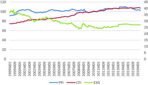
This paper explains the co-movement between the P.P.I. and C.P.I. with the exchange rate as the controlling variable using the monthly observations from 1999:01 to 2016:12. The sources of the data are the O.E.C.D. and the Czech Statistical Office. The P.P.I. is the average price of goods and services at the first level of production, and the C.P.I. is measured from the consumer perspective, defined as the change in the price of goods and services to the consumer over time. The Czech statistical office calculates the C.P.I. and P.P.I. by using the Laspeyres index. It is equivalent to the observed monthly C.P.I. and P.P.I. (2010 = 100), the percentage change in the same period from previous years, and percentage changes from the previous period. The exchange rate is the monthly exchange rate between the Czech Republic and the euro. Our data are not seasonally adjusted because the base of our P.P.I. and C.P.I. data is (2010.=.100), which helps to make more-precise comparisons. The data lack significant variation and thus need not be seasonally adjusted. Table 1 illustrates descriptive statistics for the P.P.I., C.P.I. and exchange rate of the Czech Republic; all of the variables represent positive mean and median. The C.P.I. shows the highest and the exchange rate the lowest volatility. The skewness of the P.P.I. and C.P.I. are negative; thus, series are skewed to the left whereas the exchange rate skews to the right. The kurtosis of the C.P.I. and exchange rate are less than 3, resulting in a platykurtic distribution, which designates lower volatility. However, the kurtosis for the P.P.I. is greater than 3-termed leptokurtic, implying higher volatility. The Jarque Bera test indicates that the variable is non-normally distributed.

Table 1. Descriptive statistics of the variables of the Czech Republic.

Variables	Mean	Maximum	Minimum	Std. Dev.	Skewness	Kurtosis	Jarque Bera
P.P.I.	102.452	110.5	91.1	3.917	−0.459	3.598	10.687***
C.P.I.	93.486	108.5	74.5	10.891	−0.108	1.597	17.878**
E.X.G.	28.951	38.834	23.894	3.730	0.765	2.570	22.436***

Note: *** indicate significance at the 0.01 level.

Source: Authors’ calculation.

This study uses C.Z.K. against the euro due to the adoption of the euro as new currency by the E.U. in January 1999. The period is critical to evaluate the co-movement between the P.P.I. and C.P.I. concerning the exchange rate. The rate becomes more important in a small open economy such as the Czech Republic. The exchange rate passes through inflation in two ways. In the first channel, it has a direct effect on the price of the imported goods that are intended to be used as raw materials in the consumer market and to produce goods (Schröder & Hüfner, 2002). In the indirect channel, the exchange rate affects the economy through aggregate demand and changes the output (Laflèche, 1997). The Czech Republic started inflation targeting in 1998 after the currency crisis of 1997. The immediate effect of the monetary policy was successful, and inflation declined rapidly in 1998. In the 1999–2002, the economy witnessed improvement assisted by a massive inflow of foreign investment, which caused a substantial appreciation of the exchange rate. In the following period, from 2003–2005, unemployment dropped, and a trade surplus was recorded. The significant downturn in C.P.I. was observed due to a slowdown in the P.P.I. and indirect taxes. The Czech Republic joined the E.U. in 2004, which had a positive effect on the overall macroeconomic state and further improved the inflow of foreign investment.

The data indicate several fluctuations over the time, particularly in 1997–2001, when the C.Z.K. depreciated. In the subsequent period (2002–2009), the C.Z.K./E.U.R. exchange rate appreciated. The Czech Republic converted the managed floating system to the flexible exchange rate system in 1997 (Josifidis et al., 2009). After the global financial crisis in 2009, the exchange rate depreciated and showed considerable fluctuation. The C.P.I. touched the negative level, and the P.P.I. witnessed a declining trend in 2008–2009. To control the situation, the C.R.B. reduced the interest rate. In 2013, the C.Z.K. was devalued to reduce the import price and enhance the demand for domestic products, which resulted in a low C.P.I. At the same time, the P.P.I. declined due to the falling oil prices. The flat trend in both C.P.I. and P.P.I. remained, whereas the C.Z.K./E.U.R. exchange rate position was weak in 2015–2016. We can conclude from the above analysis that structural changes occurred (Figure 1).

Figure 1. Trends of P.P.I., C.P.I. and exchange rate.

Source: Authors’ calculation.

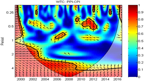
The empirical results about the relationship between the P.P.I. and C.P.I. are reported in Figure 2. The co-movement and causation relationship examines the period from 2003:10 to 2005:10, in which the C.P.I. leads the P.P.I.; the arrows pointing to the left and up indicate the anti-phase relationship, with an average coherency of 0.7 and a 0.25–0.5 year frequency. The analysis validates the existence of a short-term effect of C.P.I. on the P.P.I. (Tiwari et al., 2014). During the period, the Czech economy recorded rapid growth primarily caused by consumer demand, which was reflected in the increasing household disposable income. The weak external demand, growth in regulated prices and the fiscal policy had a favorable effect on the balance of trade. During the period, the P.P.I. subsequently increased because of the changes in indirect taxes and food and energy prices. Demand-pull inflationary pressures remained low due to the highly competitive environment of the retail market. However, from 2006:08 to 2008:02, we observe a brief effect of the P.P.I. on the C.P.I., the arrows directing to the right and up suggesting that the variables are in-phase with positive effect (Ulke & Ergun, 2014). During this period, the C.P.I. continued rising due to food prices and indirect taxes, with a similar effect on the P.P.I. From mid-2008 until 2011, both the C.P.I. and P.P.I. moved together, showing no lead-lag relationship as both declined due to the uncertainty prevailing at the global level. The situation continued to the end of 2011, when the economic recovery started and led to a state of stability. In the next period, 2011:10 to 2014:04, arrows point to the left and down, meaning that the P.P.I. is leading the C.P.I. with an average coherency of 0.7 at a 0.25–0.5-year frequency. The lower frequency implies that the P.P.I. influenced the C.P.I. in the long-term (Sidaoui, Capistrán, & Chiquiar, 2009). At the same time, the Czech economy was passing through the most prolonged recession in the country’s history, largely due to weakening domestic and foreign demand. The economy contracted due to external and domestic household demand and government consumption, which caused a budget deficit and falling wages and exerted downward pressure on prices. These developments simultaneously resulted in the low P.P.I. (Skořepa et al., 2016).

Figure 2. Co-movement between the P.P.I. and C.P.I.

Note: Cross wavelet coherency between the P.P.I. and C.P.I. The thick black contour indicates the 5% significance level against the red noise, which is assessed from the Monte Carlo simulations by the phase randomized surrogate series. The blue color indicates low coherency, whereas the red color designates high coherency. The arrows illustrate the phase difference, In-phase directing right, anti-phase guiding left. In-phase relationships with P.P.I. leading (lagging) C.P.I. point up (down) and to the right. Anti-phase relationships with P.P.I. leading (lagging) C.P.I. point down (up) and to the left.

Source: Authors’ calculation.

In Figure 3, the finding illustrates that the P.P.I. and exchange rate have a noteworthy association with various periods including 2002:10 to 2003:10, 2005:02 to 2007:02, 2007:08 to 2010:05 and 2012:08 to 2015:02. From 2002:10 to 2003:10, the arrows are pointing to the left and up, and the exchange rate is leading the P.P.I. with an average coherency of 0.7 and a frequency band of 0.2–0.5. The massive capital inflow and appreciation of the C.Z.K. increased the P.P.I. From 2005:02 to 2007:02, the arrows pointing to the right and up indicate that the P.P.I. is leading the exchange rate positively, with an average coherency of 0.6 and a frequency band 0.2–1. In the period, the P.P.I. has a leading role in the exchange rate, which is consistent with the results of An and Wang (2012), which state that the P.P.I. causes the exchange rate. C.Z.K. appreciation driven by the current account improvement and capital inflow made imports cheaper, particularly in energy-related materials. This saving helped to minimise the effect of the rising cost of raw materials on the world market and keep the P.P.I. low in the short-term.

Figure 3. Co-movement between the P.P.I. and exchange rate.

Note: Cross wavelet coherency between the P.P.I. and exchange rate. The thick black contour indicates the 5% significance level against the red noise, which is assessed from the Monte Carlo simulations using the phase randomized surrogate series. The blue color indicates low coherency, whereas the red color designates high coherency. The arrows illustrate the phase difference, In-phase directing right, anti-phase guiding left. The arrows directed up (down) and to the right indicate that the P.P.I. is leading (lagging) the exchange rate. The arrows toward down (up) and to the left suggest that P.P.I. is leading (lagging) the exchange rate.

Source: Authors’ calculation.

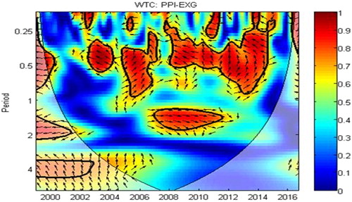
From 2007:08 to 2010:05, the exchange rate led the P.P.I. positively with an average coherency of 0.8 across a 0.25–0.5-year frequency band. The arrows are pointing up and left, suggesting an anti-phase relationship between the variables. The outcome is in line with Skořepa et al. (2016), who notice that the exchange rate leads the P.P.I. The exchange rate in the period witnessed an appreciation trend due to the favorable economic conditions along with the decreasing current account deficit and foreign short-term investment. In this period, due to greater imports and to the level of external demand, we noticed an increase in production costs at the domestic level, which translated into the dynamics of the P.P.I. The period is characterised by tremendous economic growth and exchange rate appreciation (Maria-Dolores, 2008). The main reason for this appreciation is the result of the “carry trade”, which makes the C.Z.K. most attractive to investors due to the precarious financial crisis. The exchange rate also appreciated in 2007–2008 because of short-term foreign investment and a narrowing of the negative interest rate differential against the euro, in addition to economic growth and a trade surplus. The result indicates that the exchange rate affected raw materials prices, which ultimately affected the P.P.I. Thus, the exchange rate exerted an upward pressure on the P.P.I. However, in 2008, the external demand declined, and the C.Z.K. depreciated. In mid-2009, the economy contracted due to a fall in demand from trading partners. The price dropped in all of the sectors of the P.P.I. in 2009 due to declining input prices at the domestic and international levels. Moreover, from 2009 to 2010, the P.P.I. started decreasing due to the global financial crisis of 2008; the main reason for this decrease was the prices of essential commodities (Su, Khan, et al., 2016). However, from 2012:08-2015:02, arrows directing to the left and up indicate that the exchange rate caused the P.P.I. to have an average coherency of 0.8 across a 0.25–1-year frequency band. The economy improved, and the P.P.I. witnessed a slightly increasing trend during this time. In November 2013, the C.R.B. devalued the C.Z.K. to increase exports and employment, but this measure caused rising inflation. The deliberate depreciation was intended to raise the price of domestic goods and increase external demand.

Figure 4 indicates the C.P.I. and exchange rate results, which show that both have a significant effect in several periods: 2002:04 to 2003:05, 2007:01 to 2010:02 and 2011:05 to 2013:08. From 2002:04 to 2003:05, the exchange rate led the C.P.I., with an average coherency of 0.9 and a 0.1–0.25-year frequency band consistent with Zhu (2012), which suggests that variations in the exchange rate caused C.P.I. The arrows direct left and up, suggesting an anti-phase relationship between the variables. During the period, the C.P.I. declined, the labor market situation improved, the C.Z.K. appreciated, and there was a reduction in the current account deficit. The effect of the exchange rate on the C.P.I. from 2002:04 to 2003:05 is high in frequency, which indicates a short-term relationship (Coricelli, Jazbec, & Masten, 2006).

Figure 4. Co-movement between the C.P.I. and exchange rate.

Note: Cross wavelet coherency between the C.P.I. and exchange rate. The thick black contour indicates the 5% significance level against the red noise, which is assessed from the Monte Carlo simulations using the phase randomized surrogate series. The blue color indicates low coherency, whereas the red color designates high coherency. The arrows illustrate the phase difference, In-phase directing right, anti-phase guiding left. The arrows directed up (down) and to the right indicate that the C.P.I. is leading (lagging) the exchange rate. The arrows toward down (up) and to the left suggest that the C.P.I. is leading (lagging) exchange rate.

Source: Authors’ calculation.

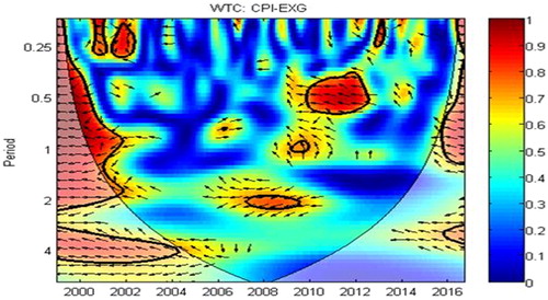
Conversely, the relationship takes a reverse form from 2007:01 to 2010:02, and the C.P.I. started leading the exchange rate. The arrows point to the left and down, suggesting that the C.P.I. is leading the exchange rate with an average coherency of 0.4 across the 1–3-year frequency band. The low frequency implies a short-term effect of C.P.I. on the exchange rate. The results are consistent with Su, Khan, et al. (2016), who reveal that the C.P.I. Granger causes the exchange rate. In mid-2007, the C.P.I. increased along with other macroeconomic variables such as interest rate and employment. However, at the end of 2007, the C.Z.K. appreciated due to improvement in the output balance, increasing the supply of foreign currency in the market (Antal, Hlaváèek, & Holub, 2008). The other factor includes a shifting of short-term investment because of the financial market turbulence; investors shift their investment from risky Dollar assets to the secure one. The exchange rate depreciated, driven by the unpredictability that prevailed at the global level. In 2009, the Czech Republic passed through a period of recession, which resulted in an exchange rate depreciation and falling C.P.I. However, at the start of 2010, the economy began recovering, and the C.P.I. increased due to the net export of food and to energy prices (Nalban, 2015). From 2011:05 to 2013:08, arrows point down and to the right, showing that variables have an in-phase connection and that the exchange rate leads the C.P.I. The economy recovered, and the price indices saw a slightly increasing trend during this time. The C.P.I. decreased, largely driven by administrative prices such as indirect taxes. In 2013, the C.R.B. devalued the C.Z.K. to boost exports and employment, but this measure resulted in rising inflation. The deliberate depreciation aimed to increase the price of domestic goods and external demand.

Figures 3 and 4 show that the exchange rate contributes to the evolution of both the C.P.I. and P.P.I. consistent with the work of Nalban (2015), which explains that the exchange rate plays a significant role in both price indices. The finding signifies the presence of structural changes in the full sample, which made the estimation unstable in the long-term. The connection between the P.P.I. and C.P.I. exists in 2004 to 2005, 2007 to 2010 and 2012 to 2014, indicating that the exchange rate plays a significant role in the relationship between the P.P.I. and C.P.I. In the same period, the Czech economy flourished with the positive development of attaining low interest rates, decreasing the current account deficit and increasing short-term investment. In the short-term, the C.P.I. changes according to the P.P.I. Nevertheless, in the remaining period, we did not notice a linkage between the P.P.I. and C.P.I. However, after controlling for exchange rate, the relationship changes from the previous outcomes. Figure 5 reveals the co-movement and causation between the P.P.I. and C.P.I. when the exchange rate is restrained. The relationship between the C.P.I. and the P.P.I. from 2002:04 to 2007:06 reveals a high-intensity co-movement with an average frequency band of 0.8. This co-movement shows that during this period, the Czech P.P.I. and C.P.I. had a strong relationship over the short-term (Su, Khan, et al., 2016). From 2002:04 to 2007:06, the C.P.I. is leading the P.P.I., and the positive relationship becomes greater compared with previous results. Nevertheless, at the beginning of the period, the C.P.I. affects the P.P.I. at a higher frequency, which later diminishes. In the next phase from 2007:06 to 2015:08, the P.P.I. starts driving the C.P.I. (Hájek and Horváth, 2015). The P.P.I. Granger affects the C.P.I. with a coherency of 0.25 to 1.5, which implies a long-term relationship and suggests that when the exchange rate effect is included, the link between the P.P.I. and C.P.I. is more stable and that the period of association appears long. Based on the previous outcomes stated in Figure 2, we observe that from 2011 to 2014, the C.P.I. affects the P.P.I. However, in Figure 5, the relationship reversed, and the P.P.I. started to affect the C.P.I. at a lower frequency in the case of the exchange rate as controlling variable. The period from 2011 to 2014 was considered a recovery phase, but at the external sector level, demand and the exchange rate remained flat. When the effect of the exchange rate is reduced, the P.P.I. importance is increased because the import price was previously the main driving power of the C.P.I. The analysis reveals that the link between the P.P.I. and C.P.I. appears long and reverses when the exchange rate is controlled.

Figure 5. Co-movement between the P.P.I. and C.P.I. and exchange rate as a controlling variable.

Note: Wavelet partial coherency between the P.P.I., C.P.I. and exchange rate is the controlling variable. The thick black contour indicates the 5% significance level against the red noise, which is assessed from the Monte Carlo simulations using the phase randomized surrogate series. The blue color indicates low coherency, whereas the red color designates high coherency. The arrows illustrate the phase difference, In-phase directing right, anti-phase guiding left. The arrows directed up (down) and to the right indicate that the P.P.I. is leading (lagging) C.P.I. The arrows toward down (up) and to the left suggest that the P.P.I. is leading (lagging) the C.P.I., whereas the exchange rate is utilized as a control variable.

Source: Authors’ calculation.

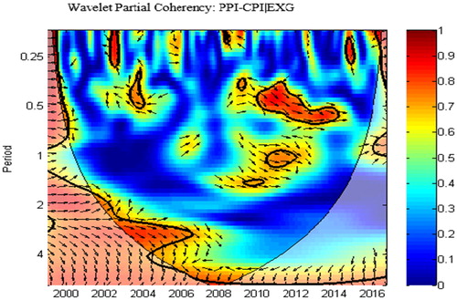
However, once the effect of the exchange rate is restrained, the direction of causality changes, running from P.P.I. to C.P.I., and the period extends from 2007:06 to 2015:08. The exchange rate remained a crucial element in the formation of inflation from 2007:06 to 2015:08, particularly during the financial crisis in 2008 and the eurozone debt crisis. The result indicates that the P.P.I. and C.P.I. have time-changing co-movement over the time and frequency domain. The exchange rate has a significant contribution in explaining both the P.P.I. and C.P.I. When the exchange rate varies, we notice reflections in the import prices, which are eventually passed on to the C.P.I. and P.P.I. Depreciation in the exchange rate makes exports cheaper and increases the cost of imports, which causes an increase in aggregate domestic demand. This development on the demand side will finally lead to higher production costs, labor, and wages, which ultimately cause an increase in domestic prices (Laflèche, 1997; Schröder & Hüfner, 2002). Conversely, when the currency appreciates against the other currency, imports become cheaper; thus, exports and aggregate demand will fall, which consequently causes price levels to decline. Figures 3 and 4 report that in the short-term from 2003 to 2006, the exchange rate Granger affects both the P.P.I. and C.P.I. The main reason is the strengthening of the C.Z.K., which makes the P.P.I. and C.P.I. rise (Josifidis et al., 2009). We did not detect a significant relationship in the remaining period. However, holding the exchange rate as a controlling variable, we conclude that the causality between the P.P.I. and C.P.I. appears to be more stable. Previously, we observed that the lead-lags relationship between the C.P.I. and P.P.I. existed in the following periods: 2003 to 2006, 2007:10 to 2008:04 and 2011:10 to 2014. By comparing the theoretical model and the estimated finding, we observe that the explanation of the causality between the P.P.I. and C.P.I. is more sensitive to external than to internal elements of the Czech Republic. The results support the expenditure-switching model, which states that the exchange rate is reflected in the P.P.I. and C.P.I. through the intermediate input factors. At the first point, the exchange rate affects import prices, and these price fluctuations are then passed to the P.P.I. and C.P.I. The outcome shows that the C.P.I. has a more significant effect on the P.P.I.; therefore, policy makers might formulate inflation targeting with greater attention toward the C.P.I. In this logic, a proper prediction mechanism of the P.P.I. at production would help in the monitoring of inflation. The result demonstrates that the exchange rate is the major contributor in explaining the C.P.I. and P.P.I.; thus, the central bank should be more concerned about the effect of the exchange rate, which results in inflationary pressure in the country. The risk of deflation can be minimised if the central bank exchange rate intervention continues in the long-term, which provides substantial information for exporters about price adjustments due to exchange rate fluctuations.

6. Conclusion

This study examines the exchange rate role in the causality relationship between the P.P.I. and C.P.I. in the Czech Republic by using wavelet analysis. The finding of the co-movement between the C.P.I. and P.P.I. in the time domain shows a positive relationship across the period. The two variables have a relationship at higher frequencies (short-term) in the frequency domain. Once the exchange rate influence is contained, the results indicate that the time horizon of the causality appears longer. The findings support the expenditure-switching model, which explains that the exchange rate has a significant explanatory power for the C.P.I. and P.P.I. The relationship between the P.P.I. and C.P.I is sensitive to the exchange rate, which is ultimately reflected in inflation. The exchange rate plays a role in the C.P.I. and P.P.I.; therefore, the central bank should be more alarmed about the consequences of exchange rate shocks, which can cause inflationary pressures in the country. Thus, a suitable forecast instrument of the P.P.I. at production would help in the monitoring of inflation. The risk of deflation can be minimised if the central bank exchange rate intervention continues in the long-term. It can be helpful to provide considerable evidence to exporters about price adjustments due to exchange rate fluctuations. The Czech Republic utilised various exchange rate regimes over the years. The current work can be extended in the future by using a different exchange rate regime. Before 1993, the Czech Republic used a conventional fixed exchange rate with a narrow fluctuation. In 1996, the country converted to intermediate regime fluctuation margins. The floating exchange rate regime remained from 1997 to 2007. The various exchange rate regimes have different effects on the relationship between the P.P.I. and C.P.I. Examining this relationship can provide a path forward for future research by extending the current work with a new dimension of using the various exchange rate regimes.

Disclosure statement

No potential conflict of interest was reported by the authors.

Notes

1 A strategy to leverage the cross-currency situation intended to benefit from the interest rate differential and low instability. The strategy involves borrowing funds at a low interest rate in one currency and purchasing assets with a high yield. In 2007, the low interest rate and exchange rate fluctuation made the Koruna an attractive currency for trade.

2 The data set shortens by feature derivation the mean essential to precisely entitle. In this case, one must cautiously select the features to excerpt; then, the feature set delivers the pertinent information from the input data to accomplish the chosen assignment by employing a shortened demonstration rather than a full-sized one. A time series will show self-similarity if the series displays dependency (i.e., the whole series displays a similar form, such as wave and cycle) in the long-term. With the help of character and resemblance of the data, the C.W.T. excerpts the local amplitude of the time series in both the time and frequency domains. Then, the subsequent wavelet coherency and phase difference indicators are measured. Therefore, the subsequent wavelet coherency and phase difference indicators are measured to determine how the local amplitudes of the two variables link and which one causes the other.

References

- Adámek, E. (2016). Factors influencing the development of the Czech crown. Procedia-Social and Behavioral Sciences, 220(2016), 3–11.
- Adetiloye, K. A. (2010). Exchange rates and the consumer price Index in Nigeria: A causality approach. Journal of Emerging Trends in Economics and Management Sciences, 1(2), 114–120.
- Adeyemi, O. A., & Samuel, E. (2013). Exchange rate pass-through to consumer prices in Nigeria. European Scientific Journal, 9(25), 110–123.
- Aguiar-Conraria, L., Azevedo, N., & Soares, M. J. (2008). Using wavelets to decompose the time-frequency effects of monetary policy. Physica A: Statistical Mechanics and its Applications, 387(12), 2863–2878.
- Aguiar-Conraria, L., & Soares, M. J. (2013). The continuous wavelet transform: Moving beyond uni- and bivariate analysis. Journal of Economic Surveys, 28(2), 344–375.
- An, L., &Wang, J. (2012). Exchange rate pass-through: Evidence based on vector autoregression with sign restrictions. Open Economies Review, 23(2), 359–380.
- Antal, J., Hlaváèek, M., & Holub, T. (2008). Inflation target fulfillment in the Czech Republic in 1998–2007: Some stylized facts. Finance a úvěr-Czech Journal of Economics and Finance, 58(09–10), 406–424.
- Babecká-Kucharýuková, O. (2009). Transmission of exchange rate shocks into domestic inflation: The case of the Czech Republic. Finance a úvČr-Czech Journal of Economics and Finance, 59(2), 137–152.
- Baghestani, H., & Danila, L. (2014). Interest rate and exchange rate forecasting in the Czech Republic: Do analysts know better than a random walk? Finance a úvěr-Czech Journal of Economics and Finance, 64(4), 282–295.
- Balcilar, M., Ozdemir, Z. A., & Arslanturk, Y. (2010). Economic growth and energy consumption causal nexus viewed through a bootstrap rolling window, Energy Economics, 32(6), 1398–1410.
- Ball, L. (1992). Why does high inflation raise inflation uncertainty? Journal of Monetary Economics, 29(3), 371–388.
- Beblavý, M. (2007). Monetary policy in Central Europe. London, UK: Routledge.
- Bhattacharya, P. S., & Thomakos, D. D. (2008). Forecasting industry-level CPI and PPI inflation: Does exchange rate pass-through matter. International Journal of Forecasting, 24(1), 134–150.
- Bloomfield, D., McAteer, R., Lites, B., Judge, P., Mathioudakis, M., & Keena, F. (2004). Wavelet phase coherence analysis: application to a quiet-sun magnetic element. The Astrophysical Journal, 617, 623–632.
- Calvo, G., & Reinhart, C. (2000). Fear of floating. The Quarterly Journal of Economics, 117(2), 379–408.
- Coricelli, F., Jazbec, B., & Masten, I. (2006). Exchange rate pass-through in EMU acceding countries: Empirical analysis and policy implications. Journal of Banking & Finance, 30(5), 1375–1391.
- Daniela, Z., Mihail-Ioan, C., & Sorina, P. (2014). Inflation uncertainty and inflation in the case of Romania, Czech Republic, Hungary, Poland and Turkey. Procedia Economics and Finance, 15(2014), 1225–1234.
- Dube, S. (2016). Exchange rate pass-through (ERPT) and inflation-targeting (IT): Evidence from South Africa. Economia Internazionale/International Economics, 69(2), 119–148.
- Friedman, M. (1977). Nobel lecture: Inflation and unemployment. The Journal of Political Economy, 85(3), 451–472.
- Geršl, A., & Holub, T. (2006). Foreign exchange interventions under inflation targeting: The Czech experience. Contemporary Economic Policy, 24(4), 475–491.
- Grinsted, A., Moore, J. C., & Jevrejeva S. (2004). Application of the cross wavelet transform and wavelet coherence to geophysical time series. Nonlinear Process Geophysics, 11(5/6), 561–566.
- Gujarati, D. N. (1995). Basic econometrics (3rd ed.). New York, NY: McGraw-Hill International Editions.
- Hájek, J., & Horváth, R. (2015). Exchange rate pass-through in an emerging market: The case of the Czech Republic. Emerging Markets Finance and Trade, 52(11), 2624–2635.
- Holub, T., & Hurník, J. (2008). Ten years of Czech inflation targeting: Missed targets and anchored expectations. Emerging Markets Finance and Trade, 44(6), 67–86.
- Hudgins, B., Parker, P., & Scott, R. N. (1993). A new strategy for multifunction myoelectric control. IEEE Transactions on Biomedical Engineering, 40(1), 82–94.
- Imimole, B., & Enoma, A. (2011). Exchange rate depreciation and inflation in Nigeria (1986–2008). Business and Economic Journal, 28(1), 1–12.
- Ito, T., & Sato, K. (2007). Exchange rate pass-through and domestic inflation: A comparison between East Asia and Latin American countries. Research Institute of Economy, Trade, and Industry, Discussion Papers, 7040.
- Jin, X. (2012). An empirical study of exchange rate pass-through in China. Panoeconomicus, 59(2), 135–156.
- Josifidis, K., Allegret, J. P., & Pucar, E. B. (2009). Monetary and exchange rate regimes changes: The cases of Poland, Czech Republic, Slovakia and Republic of Serbia. Panoeconomicus, 58(2), 199–226.
- Khan, K., Chi-Wei, S. U., Moldovan, N. C., & Xiong, D. P. (2017). Distinctive characteristics of the causality between the PPI and CPI: Evidence from Romania. Economic Computation & Economic Cybernetics Studies & Research, 51(2), 103–123.
- Kurihara, Y. (2012). Inflation targeting and the role of the exchange rate: The case of the Czech Republic. International Business Research, 5(3), 33–39.
- Lado, E. P. Z. (2015). Test of the relationship between exchange rate and inflation in South Sudan: Granger-causality approach. Economics, 4(2), 34–40.
- Laflèche, T. (1997). The impact of exchange rate movements on consumer prices. Bank of Canada Review, 1996 (Winter), 21–32.
- Loh, L. (2013). Co-movement of Asia-Pacific with European and US stock market returns: A cross-time-frequency analysis. Research in International Business and Finance, 29(2013), 1–13.
- Lyócsa, Š., Molnár, P., & Fedorko, I. (2016). Forecasting exchange rate volatility: The case of the Czech Republic, Hungary and Poland. Finance a úvěr-Czech Journal of Economics and Finance, 66(5), 453–475.
- Mandizha, B. (2014). Inflation and exchange rate depreciation: A Granger causality test at the naissance of Zimbabwe’s infamous hyperinflation (200–2005). Economics and Finance Review, 3(9), 22–42.
- Maria-Dolores, R. (2008). Exchange rate pass-through in new member states and candidate countries of the EU. International Review of Economics & Finance, 19(1), 23–35.
- Martinez, W. O., Caicedo, E., & Tique, E. J. (2013). Exploring the relationship between the CPI and the PPI: The Colombian case. International Journal of Business and Management, 8(17), 142–152.
- McCarthy, J. (1999). Pass-through of exchange rates and import prices to domestic inflation in some industrialized economies. BIS Working Paper No. 79.
- Mohammed, K. S., Bendob, A., Djediden, L., & Mebsout, H. (2015). Exchange rate pass-through in Algeria. Mediterranean Journal of Social Sciences, 6(2), 195–201.
- Nalban, V. (2015). Exchange rate pass-through in Central and Eastern Europe: A panel Bayesian VAR approach. Finance a úvěr-Czech Journal of Economics and Finance, 65(4), 290–306.
- Ocran, M. K. (2010). Exchange rate pass-through to domestic prices: The case of South Africa. Prague Economic Papers, 4, 291–306.
- Roueff, F., & Sachs, R. (2011). Locally stationary long memory estimation. Stochastic Processes and their Applications, 121(4), 813–844.
- Schröder, M., & Hüfner, F. P. (2002). Exchange rate pass-through to consumer prices: A European perspective. Discussion Paper No. 02-20. Center for European Economic Research, Mannheim.
- Shahbaz, M., Awan, U. R., & Nasir, M. N. (2012). Producer & Consumer prices nexus: ARDL bounds testing approach. International Journal of Marketing Studies, 1(2), 78–86.
- Sidaoui, J., Capistrán, C., & Chiquiar, D. (2009). A note on the predictive content of PPI over CPI inflation: The case of Mexico. Banco de Mexico, 14, 1–18.
- Skořepa, M., Tomšík, V., & Vlcek, J. (2016). The impact of the CNB’s exchange rate commitment: Pass-through to inflation. BIS Papers Chapters, 89, 153–167.
- Su, C. W., Khan, K., Lobont, O. R., & Sung, H. C. (2016). Is there any relationship between producer price index and consumer price index in Slovakia? A bootstrap rolling approach. Ekonomicky Casopis, 64(7), 611–628.
- Su, C. W., Zhang, H. G., Chang, H. L., & Nian, R. (2016). Is exchange rate stability beneficial for stabilizing consumer prices in China? The Journal of International Trade & Economic Development, 25(6), 857–879.
- Szymańska, A. (2011). Price stability and its realization – The case of the Czech Republic and Poland. AD ALTA. Journal of Interdisciplinary Research, 1(2), 105–109.
- Tiwari, A. K. (2012). An empirical investigation of causality between producers’ price and consumers’ price indices in Australia in frequency domain. Economic Modelling, 29(5), 1571–1578.
- Tiwari, A. K., Mutascu, M., & Andries, A. M. (2013). Decomposing time-frequency relationship between producer price and consumer price indices in Romania through wavelet analysis. Economic Modelling, 31(2013), 151–159.
- Tiwari, A. K., Suresh, K.G., Arouri, M., & Teulon, F. (2014). Causality between consumer price and producer price: Evidence from Mexico. Economic Modelling, 36(2014), 432–440.
- Torrence, C., & Compo, G. (1998). A practical guide to wavelet analysis. Bulletin of the American Meteorological Society, 79(1), 61–78.
- Torrence, C., & Webster, P. J. (1999). Interdecadal changes in the ENSO-monsoon system. Journal of Climate, 12(8), 2679–2690.
- Triandafil, M, C., Brezeanu, P., Huidumac, C., & Triandafil, A. M. (2011). The drivers of the CEE exchange rate volatility-empirical perspective in the context of the recent financial crisis. Journal for Economic Forecasting, 1(2011), 212–229.
- Uddin, K.M.K., Quaosar, A.A., & Nandi, C.D. (2014). The impact of depreciation on domestic price level of Bangladesh. Journal of Economics and Sustainable Development, 5(25), 108–114.
- Ulke, V., & Ergun, U. (2014). The relationship between consumer price and producer price indices in Turkey. International Journal of Academic Research in Economics and Management Sciences, 3(1), 205–222.
- Zhou, J. (2010). Comovement of international real estate securities returns: A wavelet analysis. Journal of Property Research, 27(4), 357–373.
- Zhu, B. (2012). Exchange rate and price: A Granger causality test of consumer price index in China. In H. Tan (Ed.), Technology for Education and Learning. Advances in Intelligent Systems and Computing. Berlin, Heidelberg: Springer.