System dynamics model of crises in small and medium enterprises

Abstract

The article aims to improve existing theories of business development and crisis management with a special emphasis on inner dynamics of crises in small and medium enterprises (S.M.E.s). For these purposes, combined perspectives of system dynamics, company life cycles, crisis management, resilience and business continuity management in S.M.E.s have been used. Based on data of about 554 crises from 183 companies collected in the Czech Republic, the most common crises types and their combinations have been identified using association rules mining method. Then, a simulation system dynamics model synthesizing the main findings and allowing scenario analysis to explain and avoid some of the crises in S.M.E.s has been developed for a case study of manufacturing company. Such a simulation model enriches the present knowledge and explains complex dynamics of crises in S.M.E.s in a novel way. When properly calibrated, this model could be used as a supporting tool for decision-making in manufacturing S.M.E.s.

Keywords:

• small and medium enterprises (S.M.E.)
• crisis
• business management
• system dynamics model
• simulation modelling

Subject classification codes:

• M21
• L25
• C63

Introduction

The growth of companies is a very frequent topic for discussion. Media, governments, as well as shareholders and initial public offering (I.P.O.) markets are interested in fast growing companies and lack of growth is generally perceived as a problem. In this context, each attempt to further explain and overcome obstacles to growth may be helpful, especially in relation to the recent global financial crisis and its impact on businesses.

The main goal of this study is to develop a system dynamics simulation model of occurrence of crises in S.M.E.s. Such a model can serve as decision support tool for managers dealing with various crises and as a mean of explaining crisis dynamics. The model structure development was grounded in an analysis of empirical data about 554 crises from 183 Czech companies where the main purpose was to identify co-occurrence of different types of crises and ways how managers were dealing with these crises. The use of such a model focused on manufacturing firms including its calibration is further demonstrated on a case study of real company and related scenario analysis. This analysis could be very helpful for the manager, e.g., to predict possible impacts of various possible managerial decisions when a certain type of crisis occurs, thus allowing to avoid causing further problems in the future.

The article is organised as follows. After introductory remarks the necessity of including both internal and external causes of organizational growth crises and the current state in developing the system dynamics model of crises in S.M.E.s are explained in the literature review section. In the third and fourth parts of the article, used methodology and the empirical data analysis are presented. The fifth part introduces the company selected for the case study for which the conceptual model and then a simulation system dynamics model were developed in the sixth part. Subsequently, using the developed simulation model the analyses of two different scenarios are discussed. The final part includes concluding remarks and a list of references.

Literature review

One of the traditional approaches to the presented topic is based on analogies between natural life cycles and patterns of development in companies. In his seminal work, Larry E. Greiner (1972) started this school of thought with his five-stages model of organisational growth evolutions and revolutions. A general assumption in this approach is that companies have to go through similar stages – creativity, direction, delegation, coordination and collaboration – defined by similar problems during their growth and ageing.

A lot of further research, both theoretical and empirical, has subsequently been undertaken. Different authors (e.g., Adizes, 1988; Kazanjian, 1988; Rutherford et al., 2003; Lester et al., 2003) describe different classifications of growth stages – varying between three and 10, oriented more outwards or inwards or based on other criteria.

It is necessary to mention that although Greiner’s model is present in many management textbooks, it is not without criticism. One of the main objections is applicability of these general principles in real companies and their specific circumstances, especially in relation to causes of and solutions for various crises that may also occur concurrently and challenges in stages recognitions (Macpherson, 2005; Phelps et al., 2007). Furthermore, the organizational life cycle may be easily confounded with the business opportunity life cycle (Sull & Houlder, 2006). And another problematic issue is according to Phelps et al. (2007) that the growth stages are only linearly described.

The topic of coping with crises in S.M.E.s has gained some attention mainly due to the impact of global financial crisis on businesses. An information management tool concerning this topic combining methods from both the fields of information management and business continuity management is presented in Podaras et al. (2016). Several studies by Herbane (2010a, 2010b, 2013) have opened up this specific field and these were followed by further research related to a concept of resilience in the management of S.M.E.s (e.g., Sullivan-Taylor & Branicki, 2011; Hong, Huang, & Li, 2012) and business continuity management (e.g., Elliott, Swartz, & Herbane, 2002; Urbancová & Königová, 2011). One of the limitations of these studies is that they typically focus only on crises caused by changes in external environment, which as we think is not enough. There are also studies that deal with prediction of crisis situations or bankruptcy using financial indicators (e.g., Altman, 1983; Karas & Řezňáková, 2017).

Our argument is that it is useful to focus the research on both internal and external causes of organizational growth crises. In this way, it should be possible to model accordingly different crises under different circumstances, which is in line with previous system dynamics research in this area, related mainly to the application of system archetype Limits to Growth (Meadows et al., 1972; Forrester, 1968; Sterman, 2000; Oliva et al., 2003) or general use of system dynamics in S.M.E.s’ decision making support (Winch & Arthur, 2002; Bianchi, 2002).

The first basic concept of conceptual system dynamics model to explain the dynamics of crises was presented and discussed in conference paper (Vojtko et al., 2015). However, only a basic frequency analysis of crises and a simple causal loop diagram of company crises development were presented here.

This article builds on the previous knowledge and extends it further especially concerning the simulation model for company crises development. The below presented simulation system dynamics model synthesizes the previous findings with the findings gained by the authors of this article in a novel way. In the form of case study of manufacturing company, the simulation model has been developed allowing scenario analysis to explain and avoid some of the crises in S.M.E.s.

Methodology and data

The empirical data for the study were gathered in several stages between April and October 2014 in the form of face to face qualitative interviews with management representatives in the Czech companies (Vojtko et al., 2015). The data set covers narrative description of 183 companies and their selection of at least three of their most important crises, i.e., situations threatening their very existence in the past.

The companies were selected in a way to have broad coverage of all main industries according to the CZ NACE classification as well as of companies of different sizes – the sampling was purposeful to allow us to build a model covering all important aspects of crises development in different circumstances. The companies also vary according to number of employees (ranging from 0 to more than 100, where each category contains at least 13 companies), legal entity (the only missing type is public partnership), yearly revenue (ranging between 0.05 and 1300 million CZK, i.e., between 0.002 and 52 million EUR, with mean value 68.01 million CZK, i.e., 2.72 million EUR, and median value 10 million CZK, i.e., 0.4 million EUR) and a status of family firm (42.08% claim to be a family firm).

The data set consists of 183 companies and 554 crises with the following characteristics (see Table 1).

Table 1. CZ NACE distribution of companies in the data set.

Section	Value Label	Frequency	Valid Percent
A.	Agriculture, forestry and fishing	12	6.56
B.–E.	Manufacturing and processing	47	25.68
F.	Construction	19	10.38
G.	Wholesale and retail trade	36	19.67
H.	Transporting and storage	3	1.64
I.	Accommodation and food service activities	15	8.20
J.	Information and communication	8	4.37
K.	Financial and insurance activities	3	1.64
L.	Real estate activities	5	2.73
M.	Professional, scientific and technical activities	13	7.10
N.	Administrative and support service activities	2	1.09
P.	Education	5	2.73
Q.	Human health and social work activities	3	1.64
R.	Arts, entertainment and recreation	10	5.46
S.	Other services activities	2	1.09
	Total (N)	183	100.00

Source: Authors’ calculation.

It is clear that nearly all CZ NACE types of activities are present in the data set. The only missing ones are those that are not very common amongst S.M.E.s in the Czech Republic, i.e., the O-section (Public administration and defense), T-section (Activities of households as employers), and U-section (Activities of external organizations and bodies).

Based on the above mentioned characteristics it is possible to assume the data set covers broad range of different types of companies in different circumstances and should provide a basis for induction and model building. In addition, its structure seems to be, with some limitations, broadly representative to the whole population of S.M.E.s.

The textual descriptions of crises were categorized later which has revealed 19 specific crises features. All these features were further analysed to explore their combinations and co-occurrence – descriptive statistics, cross-tabulation and association rules mining according to Hahsler, Buchta, Gruen, Hornik, & Borgelt (2016) have been used for these purposes. These analyses have been done using M.S. Excel and R software package.

After this empirical data inquiry, a conceptual and later simulation model were developed using causal loop diagram technique and model building methodology from the system dynamics discipline (Forrester, 1992; Sterman, 2000; Mildeová & Dalihod, 2017). Vensim modelling environment has been used both for conceptual as well as simulation model development.

This simulation model represents a dynamic theory of causal relationships between various elements of company behaviour as well as external influences and aims to explain mechanisms of how different crises can occur. With such a model, testing of different policies dealing with crises under various circumstances can be done when calibrated for given conditions.

For the simulation model testing, calibration and scenario analysis, one company from the data set has been selected as a case study of typical representative from a group of manufacturing firms with the most common crisis features found. This allowed exploring the dynamics in more detail and evaluating validity of the model in comparison to the known real company behaviour. The final model including all mathematical relationships and calibration is available online (https://goo.gl/1VH5XV) and can be re-calibrated or extended for other cases.

Data analysis

The data analysis for the purpose of this study consists of the three steps – the basic frequency analysis, the cross tabulation analysis, and the association rules mining.

Basic frequency analysis

Nineteen specific crises features were specified under the study (see C1 to C19, sorted in descending order of frequency of occurrence in Table 2).

Table 2. Crisis features frequencies according the surveyed sample (N = 183).

Crisis feature	Valid percent
Employees (C13)	46.45
Customers/demand (C6)	42.62
Inputs and supplies (C1)	28.42
Regulations, bureaucracy, taxes (C4)	27.32
Collecting bills (C5)	25.68
Competition (C3)	20.77
Owners (C12)	16.94
Financial capital (C2)	15.85
Capacity (C10)	14.21
Natural disasters (C11)	10.93
Technical breakdown (C19)	10.38
Selling prices (C7)	8.74
Quality of production (C16)	8.20
Entrepreneur – personal crisis (C8)	7.10
Thefts (C18)	6.56
Placement of business (C14)	6.01
Processes (C9)	3.83
Outdated product (C15)	1.09
Legal entity (C17)	1.09

Source: Authors’ calculation.

The most common crisis features in the surveyed businesses were those related to: (1) employees (C13); and (2) customers/demand (C6) – this category was, based on the interviews, related mainly to the global financial crisis and subsequent demand shock. In the second distinctive group the crisis features roughly represent one quarter of cases each. These are: (1) inputs and supplies (C1) – their quality, availability and prices; (2) regulations, bureaucracy and taxes (C4); (3) collecting bills (C5); and (4) competition (C3). All four are linked to the external environment. Other crisis features are less common, i.e., their frequency was less than 20%. Nevertheless when combined with more frequent crises their impact might be significant as well.

Cross tabulation analysis

We have further analysed the data using cross tabulations (see Vojtko et al., 2015, for more detail) which has revealed some statistically significant differences as tested by χ² test on α = 0,1 (higher α has been chosen due to exploration nature of this analysis) between the following variables in the data set:

• Engagement in international business (inputs and supplies, outdated product, quality of production);

• CZ NACE and crisis features (competition, collecting bills, selling prices, owners, employees, placement of business, outdated product);

• Knowledge intensity of a business (high or low knowledge intensive industry, services or agriculture/construction) and crisis features (selling prices, capacity);

• Written strategy and crisis features (financial capital).

This shows that factors like the type of industry, the knowledge intensity, and the international scope could play a crucial role in understanding of crises in companies and it would be meaningful to respect these differences also in the modelling process accordingly, i.e., to reflect them either in the model structural properties or during the calibration.

Association rules mining

To further examine significance of relationships between occurrences of different crises within a company, association rules mining has been used (for more detail about using association rules see, e.g., Rolínek et al., 2015). Several interesting relationships explaining the three most frequent crises were identified by this approach – inputs and supplies (C1), customers/demand (C6) and employees (C13). No other rules have been found to explain the co-occurrence among the other types of crises. The analysis has revealed the following rules explaining co-occurrence with crises C1, C6 and C13, as shown in Table 3.

Table 3. Association rules.

	lhs		rhs	support	confidence	lift
Set I	{C16 = Yes}	= >	{C1 = Yes}	0.05464481	0.5555556	1.955128
Set II	{C16 = Yes}	= >	{C6 = Yes}	0.06557377	0.6666667	1.311828
	{C10 = Yes}	= >	{C6 = Yes}	0.08196721	0.6250000	1.229839
	{C3 = Yes}	= >	{C6 = Yes}	0.13661202	0.5681818	1.118035
	{}	= >	{C6 = Yes}	0.50819672	0.5081967	1.000000
	{C1 = Yes}	= >	{C6 = Yes}	0.14207650	0.5000000	0.983871
Set III	{C18 = Yes}	= >	{C13 = Yes}	0.06010929	0.7333333	1.443011
	{C16 = Yes}	= >	{C13 = Yes}	0.07103825	0.7222222	1.421147
	{C2 = Yes}	= >	{C13 = Yes}	0.12021858	0.6285714	1.236866
	{C10 = Yes}	= >	{C13 = Yes}	0.08196721	0.6250000	1.229839
	{}	= >	{C13 = Yes}	0.50819672	0.5081967	1.000000

Source: Authors’ calculation.

The association rules mining has shown the highest lift (i.e., measure of performance of right hand side rule – rhs – in predicting left hand side – lhs) for the inputs and supplies crisis (C1) and quality of production crisis (C16). The value of 1.96 means that occurrence of both crises is approximately twice more likely than random. When further tested by χ² test, only this relationship (C1 vs C16) was statistically significant (χ²= 7.2293, df = 1, p-value =0.007172).

Another set of association rules has been found to explain the crisis related to customers and demand (C6). In this case, the crises with lift >1 are again quality of production (C16), capacity (C10) and competition (C3).

The last set of association rules explains employee crisis (C13). This crisis was the most frequent one in the dataset occurring in more than 46% of interviewed companies. Other crises related to this one are thefts (C18), quality of production (C16), financial capital (C2) and capacity (C10).

Summary findings from the data analysis

Previous analyses show some underlying patterns in the occurrence of crises. Mainly the crises related to employees (C13), customers (C6) and inputs and supplies (C1) co-occur more probably with some others.

Even though we cannot assume directly that these associations in data describe causal relationships (due to the impact of macro factors on many companies during their existence, as example), we should try to explain the crises occurrence and develop coherent theory.

It is also obvious from the crises features designation that some of them are more related to internal processes or policies (e.g., C13, C10, C16) and others to external environment (e.g., C1, C6, C3). Thus, it is necessary to choose a methodological approach for the proper explanation of crisis occurrence and development. That way we could combine these two points of view together. It would allow us to test the different policies to deal with certain crises, and to avoid unwanted consequences as well.

Case study

A typical representative for the Czech manufacturing industry has been selected from the data set for the case study. The selection criteria were: (1) belonging to the most common CZ NACE category (B-E Manufacturing and Processing with 25.7% companies in the sample); and (2) co-occurrence of the most common crisis features found (C6, C13).

This company with approximately 200 employees produces automotive parts predominantly for trucks. In this company, two main crises according to the above described categorisation have occurred – customers/demand (C6) and employees (C13). The first one was, according to interviews, related to the global financial crisis and overall drop in demand in 2009–2011. The second one has started later and mainly is related to the lack of qualified employees and problems with production quality.

Both crises also showed secondary effects similar to the ones the association rules mining has revealed. Especially the crisis related to employees has increased problems with quality of production (C16) as well as with capacities (C10).

Some effects and dependencies observed in the company chosen for the case study will be used in the following chapters mainly to explain or demonstrate the below described relations.

System dynamics model of crises development

To show the dynamics of such a crisis development in its complexity we have developed at first a conceptual model that should reflect the most relevant relationships on a selected case study of a manufacturing company (Vojtko et al., 2015), and then a system dynamics simulation model.

Methodologically the model synthesises the knowledge from the data set and interviews and uses building blocks previously developed at MIT (Sterman, 2000). The process of such a model development and use generally follows the next steps (Forrester 1992): (1) setting the purpose and scale; (2) dynamic hypotheses definition – conceptual model; (3) simulation model definition; (4) model testing and evaluation; and (5) explanation of the model dynamic behaviour, testing of policies and finding solutions of consecutive problems. The stock-and-flow diagram of the simulation model is shown in the Figure 1.

Figure 1. System dynamics model for company crises development.

Source: own

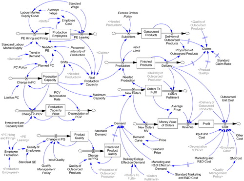
In this diagram, the single line arrows describe proposed causal relationships between different variables (‘ǁ’ symbol on the arrow means delayed effect), rectangles represent stock variables (levels, reservoirs), and double line arrows represent flows that change the values of stock variables over time.

The diagram of the simulation model contains hard and soft variables and provides the necessary holistic view that should allow exploration of proposed main causal relationships as well as an analysis of feedback structures (in other words vicious/virtuous or balancing/goal seeking cycles – dynamic hypotheses). After mathematical definition of all relationships and model calibration we are able to calculate the logical consequences of different scenarios and management policies related to crises.

This model has been purposefully calibrated with data about the chosen company for the time horizon of 10 years to be able to see long-term consequences. The time step being used is one week, which allows modelling of processes on various relevant time scales (weeks, months, years). Its borders and structure were selected according to the factors revealed in the interviews with company managers, through the data analysis of crises and financial statements of the company, and literary review (system dynamics, management, economics).

This particular system dynamics model describes relationships among the following major factors related to the crises development:

• number of production employees and labour market

• technological production capacity (in natural as well as financial units)

• production

• outsourced production (including prices/cost)

• stock of finished products

• product quality (ranging from 0 = lowest to 1 = highest possible) and claims

• inputs and supplies (limitations in natural units, purchasing input prices)

• demand relative to offered prices, competition and previous investments in quality, delivery delays, research & development and marketing

• orders (in natural as well as financial units) and their fulfilment

• revenue, costs and profit

To be able to mirror the patterns of behaviour of this company during the crisis, the simulation model has been calibrated to be proportionally consistent with the case study data (namely with the number of employees, capacity, average sales, costs and profit). One of the main goals of the initial calibration was to put the model in a balanced state (base scenario). Then, this base scenario can be diverted by either external environment or internal management policies changes. When comparing the base scenario with the ones containing induced changes we would be able to quantify and test their effects.

To explain the model in further detail, we can show, as example, how the sub-model dealing with production employees works. Stock variable Production Employees (PE) is computed in the time step T by the following formula (1): (1) $${\mathit{\text{Production}}\mathrm{}\mathit{\text{Employees}}}_T=\underset{T_0}{\overset{T}{\int }}{\mathit{\text{Production}}\mathrm{}\mathit{\text{Employees}}}_{T_0}+\left({PE\mathrm{}\mathit{\text{Hiring}}}_t-{PE\mathrm{}\mathit{\text{Leaving}}}_t\right)dt$$(1) where T₀ is the first step of simulation. Thus, this variable contains the actual number of production employees in each time step (as system dynamics deals with continuous variables, we use integral representation in the model, i.e., it may not necessarily by a discrete number).

PE Hiring and Firing is dependent in the model on variables Needed PE, Production Employees, Standard Labour Market Supply and Labour Market Supply Curve. The formula for computation of its value in the time step T is shown below as (2): (2) $${PE\mathrm{}\mathit{\text{Hiring}}\mathrm{}and\mathrm{}\mathit{\text{Firing}}}_T=MI\mathrm{N}({\mathit{\text{Labour}}\mathrm{}\mathit{\text{Market}}\mathrm{}\mathit{\text{Supply}}\mathrm{}\mathit{\text{Curve}}}_T\text{*}{S\hspace{0.17em}\text{tan}\hspace{0.17em}\mathit{\text{dard}}\mathrm{}\mathit{\text{Labour}}\mathrm{}\mathit{\text{Market}}\mathrm{}\mathit{\text{Supply}}}_T,\mathrm{}IF\mathrm{}\mathit{\text{THEN}}\mathrm{}\mathit{\text{ELSE}}({\mathit{\text{Needed}}\mathrm{}PE}_T>{\mathit{\text{Production}}\mathrm{}\mathit{\text{Employees}}}_T-{\mathrm{}PE\mathrm{}\mathit{\text{Leaving}}}_T,\mathrm{}1,\mathrm{}0.1)\mathrm{}\times \mathrm{}({\mathit{\text{Needed}}\mathrm{}PE}_T-{\mathit{\text{Production}}\mathrm{}\mathit{\text{Employees}}}_T+{PE\mathrm{}\mathit{\text{Leaving}}}_T))$$(2) where Labour Market Supply Curve_T together with Standard Labour Market Supply_T represent actual labour supply for offered wage and the difference between Needed PE_T and Production Employees_T reflects how many employees are necessary to hire. If we put the whole idea in a simple way, hired employees are limited either by how many we need or how many are available on the labour market for offered wage. When firing employees, the adjustment is slower due to the avoidance of managers to do it unless necessary, and so there is only 10% change per week.

We can proceed further in the explanation to the variable PE Leaving. We can assume that due to the aging of employees and other reasons like moving away, there is going to be a constant outflow of them (0.15% per week, i.e., 7.8% per year). And this constant rate is going to be increased or decreased based on differences between standard wages on the labour market and wages being offered by the employer. Thus, such a relationship could be defined by the following formula (3): (3) $${PE\mathrm{}\mathit{\text{Leaving}}}_T=\mathit{\text{ZIDZ}}\left({\mathit{\text{Average}}\mathrm{}\mathit{\text{Wage}}}_T,\mathrm{}{\mathit{\text{Standard}}\mathrm{}\mathit{\text{Wage}}}_T\right)\times {\mathit{\text{Production}}\mathrm{}\mathit{\text{Employees}}}_T\times 0.0015$$(3) where ZIDZ is a Vensim function that divides Standard Wage and Average Wage but when Average Wage =0, returns 0 too, to avoid division by zero.

All the variables shown in the Figure 2 are mathematically expressed in a very similar manner to reflect the relationships between them – all stock variables can be expressed as integrals of differences between inflows and outflows.

Figure 2. Nonlinear relationship definition – example of labour market supply curve.

Source: own

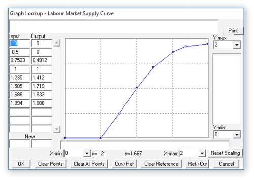
Some of the relationships should be nonlinear. The lookup functions in Vensim have been used to easily define and change these relations in the model. One example of such a relationship is shown in Figure 3 which converts ZIDZ (Average Wage_T, Standard Wage_T) to a coefficient increasing or decreasing the value of variable Standard Labour Market Supply in Formula 2 to represent the actual labour supply for average wage offered by the examined company. When the average wage to be offered is equal to the standard market wage, output of this lookup function is 1, i.e., the actual labour supply equals the standard labour market supply multiplied by 1. When the average wage is higher or lower than the standard wage, lookup function output increases or decreases faster at first and slower later. The reason for this lies in our assumption that the maximum number of available employees is limited and when the average wage to be offered is too small, nobody would be interested.

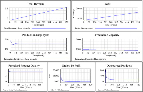
Figure 3. Results for the base scenario simulation.

Source: own

These lookup functions are just estimates deduced logically from the microeconomics theory of demand and supply. They could be easily changed when simulating scenarios to test their influence on the overall behaviour.

Several variables in the model represent external influences or policies to be applied by management and further tested by scenario analysis in relation to different crises that could occur. Their values can be easily changed in scenario definitions and the description is as follows:

• PC Policy – technological production capacity excess/deficiency with regards to demand, i.e., how much of the capacity should be kept in comparison to the long-term demand (dimensionless).

• Limit in PC – outer limit in technological production capacity, e.g., limited space etc.

• Average Wage – gross wages to be offered to production employees (CZK/month).

• Standard Wage - gross wages to be offered to production employees by competitors on the labour market (CZK/month).

• Standard Labour Market Supply – number of employees available from the labour market when Average Wage = Standard Wage (employee).

• Personnel Intensity of Production – how many units of production is one employee able to produce in a week with existing technology (units/employee/week).

• Investment per Capacity Unit – investment necessary for building new technological capacity (CZK/unit/week).

• PCV Depreciation Rate – weekly depreciation rate of production technology (dimensionless).

• Quality Management Policy – how much effort is being put into quality management quantified as a range between 0 = no effort and 1 = maximum effort (dimensionless).

• Standard QE – standard quality of hired employees quantified as a range between 0 = very low and 1 = very high (dimensionless).

• Input Quality – what is the quality of inputs and supplies quantified as a range between 0 = very low and 1 = very high (dimensionless).

• Standard Claim Ratio – proportion of claims from sold units when the product quality is lowest (dimensionless).

• Input Limit – what is the actual availability of material inputs, range between 0 = 0% and 1 = 100% (dimensionless).

• Excess Orders Policy – what proportion of excess orders in comparison to available capacity should be outsourced, range between 0 = 0% and 1 = 100% (dimensionless).

• Quality of Outsourced Products – what is the quality of outsourced products quantified as a range between 0 = very low and 1 = very high (dimensionless).

• Outsourced Unit Cost – cost per outsourced unit (CZK/unit).

• Input Unit Cost – variable cost per unit produced within the company (CZK/unit).

• Marketing and R&D cost – marketing and research/development costs aimed at increasing of demand (CZK/week).

• Standard Marketing and R&D cost – average marketing and research/development costs aimed at increasing of demand being spent by competition (CZK/week).

• QM Cost – costs induced by the quality management policy (CZK/week).

• Other Cost – all other fixed costs (CZK/week).

• Price – selling price per unit (CZK/unit).

• Standard Price – average market price per unit (CZK/unit).

• Standard Demand – number of units demanded when Price = Standard Price (units/week).

Scenario analysis

In this chapter we will describe the use of the model to create and analyse scenarios. These scenarios and their analysis could be helpful for the manager, e.g., to predict possible impacts of various possible managerial decisions when a certain type of crisis occurs. The following scenarios may be considered as examples of how to define them and interpret the results.

Base scenario

The base scenario is mainly for testing of the overall model behaviour and could serve as a basis for comparison, i.e., to quantify changes incurred in the following scenarios. For the simulation, this scenario should produce stable development of the main parameters over time. There are no changes within or outside the company and thus also the behaviour should be stable after getting to balance – demand should be balanced with the capacity.

There are several important assumptions in the model structure and calibration that should reflect the observed decision-making of managers or initial setup of main variables (variables values described below are set as for the case study company):

• For the simplification, we assume that one generic product is being produced by the company and all the calibration has been adjusted accordingly – we are using average values. If necessary, it is possible to add more detail in the model using arrays but according to our experience this would not change the overall patterns of behaviour significantly.

• Technological capacity is being kept on the level of 90% of trend in demand to avoid overinvestment; its initial state is 2500 units/week. When increasing technological production capacity, 1% of the difference between planned production capacity and actual production capacity is being added per week. When decreasing technological production capacity, 0.5% of the difference between planned production capacity and actual production capacity is being removed per week. This should reflect avoidance of managers to decrease the capacity too fast if there is a decline in demand. The overall limit for technological capacity is being set to 5000 units/week due to space limitations.

• Technological capacity is depreciated over time with the base rate 0.4% per week, approximately 18.5% per year. Because maintenance is considered to be part of other costs in this model, the depreciation is only in money value and does not harm the overall technological capacity.

• Personnel intensity of production is 37 units/employee/week.

• Initially there are 200 employees; their number is being managed according to shifts used in production (with maximum three), personnel intensity of production and production capacity. When hiring employees, all the necessary employees are hired straight away if available on the labour market. When firing employees, only 10% of excess employees are fired in a week – again, this should reflect avoidance of managers to fire employees unless really necessary. Some of the employees may also leave due to other reasons – i.e., low wages or retirement. We assume for that an initial value of 0.15% of employees per week.

• The product quality and similarly the perceived product quality are initially set to 0.85, the standard quality of newly hired employees to 0.5, quality management policy to 0.9, and input quality to 0.9 as well. The quality of outsourced products is set to 0.8. All the determinants of product quality are stable in the base scenario except employee fluctuation which takes some time to adjust from the start due to adjustments in the number of employees.

• The main effect of product quality expressed in the model is in claims. The standard claim ratio for the lowest quality is set to 0.1, i.e., 10% of deliveries. Its effect is delayed by two weeks. When the quality is higher, this ratio would drop significantly and in our case is thus less than 1.7%.

• The production per week is determined by new orders, previous unfulfilled orders and real production capacity and may be restricted by input limit, i.e., availability of input material. This limitation is being set to 1 which means that all necessary inputs are available in the right time. To get closer to reality, this input limit should be set lower. Also, there is no production above the orders, i.e., capacity is not being used to produce stock.

• When a gap exists between the orders and production capacity, it is possible to outsource a certain part of the production. This policy is being initially set to 0.5, which means that in such a case 10% of the excess orders would be outsourced per week. Outsourcing on one hand affects the overall perceived quality and costs (450 CZK/unit, i.e., 18 EUR/unit approximately) but on the other hand it may help in situations with insufficient capacity and may decrease necessary investments.

• A very important element in the model is demand. According to trends in the demand and internal policies, the capacity is being automatically managed. Demand is partially external, partially is influenced by internal policies – e.g., pricing, product quality, R&D, marketing and delays in order fulfilment. Price influence on demand is being structurally modelled in a similar way as the labour market supply, i.e., ratio between own price and standard market price is calculated and transformed to demand coefficient by a lookup nonlinear demand function. By this coefficient, standard demand is multiplied and other influences are added in the same way, but limited to maximum value of 1 – for example, if we deliver in-time it cannot increase demand, but if we deliver late there would be a negative impact on demand.

• The last part of the model deals with orders expressed in money value, revenue, costs and resulting profit. Here, an economic situation of the company is expressed in a simplified way. Again, this simplification allows seeing the main patterns of behaviour but when, for instance, crisis with cash flow would be necessary to model, it should be extended accordingly. The costs here are either variable (input unit cost is set to 400 CZK(16 EUR)/unit; outsourced unit cost is set to 480 CZK(19.2 EUR)/unit) or fixed, like depreciation of production capacity value, marketing and R&D costs (20 000 CZK(800 EUR)/week), employee cost, quality management cost (maximum 50 000 CZK(2 000 EUR)/week) and other cost (90 000 CZK(3 600 EUR)/week).

The model is being steadily adjusted from the initial to balanced state but before the end of the second year of simulation the adjustments are very small and we can neglect them (see Figure 3). Total profit being generated in the simulation is 119 million CZK, resp. 11.9 million CZK per year (i.e., €4.76 million, resp. €0.476 million per year), and revenue 1.95 billion CZK, resp. 195 million C.Z.K. per year (i.e., €78 million, resp. €7.8 million per year).

When tested in the balanced state, the variables generated by the simulation model correspond to the firm behaviour as expected – after the initial adjustments all variables became stable.

Case study crisis scenario

The second scenario deals with crises that were identified in the case study. Several changes have been made compared to the base scenario. The main one lies in the standard demand, which is now growing first and then negative demand shock and recovery occurs to reflect the global financial crisis impact.

There are also some other changes in the model calibration – a steady decrease from three to 0.5 employees available per week in standard labour market supply and steady decrease in standard quality of employees from 0.7 to 0.5 over all 10 years of simulation. These changes have been introduced to make this scenario closer to external environment factors as described in the case study.

When simulating this scenario, we should expect similar model behaviour, like the development of the case company, i.e., first the customer/demand crisis and then the crisis related to employees and quality of production.

As seen in Figure 4, the crisis scenario simulation really shows the expected behaviour which is very similar to the case study in several aspects:

Figure 4. Crisis scenario versus base scenario.

Source: own

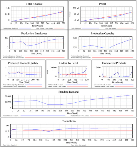
• Decrease in the demand leads to higher decrease in the number of employees than in decrease in the production capacity. This allows company to stay profitable and survive during this period.

• During the crisis, outsourcing drops and then during recovery it increases to deal with the increased demand and not enough capacity. This, again, reflects the case company behaviour successfully.

• Perceived product quality decreases over time due to the lower quality of newly hired employees, which leads to the higher claim ratio and related problems described by managers of the case study company.

For this scenario, no changes in the management policies were considered and so a question arises – what could have been done by the managers to improve the results in such situation? Or, on the contrary, what management action can cause even more problems and deepen the existing crisis?

A conclusion can be drawn from the scenario analysis and empirical data that external demand shock may be further amplified by improper management actions, especially towards employees. Thus, it would be meaningful in such situations to compensate such external shocks with better HR management, quality control, and building reserves in advance.

Conclusions and limitations

A novel way of explaining the complex dynamics of crises in S.M.E.s was presented in this article. A conceptual model reflecting the most relevant internal and external relationships of the company was developed, and subsequently, the system dynamics simulation model of occurrence of crises in S.M.E.s was used to analyse possible scenarios of specific development of the company. This enables to predict possible impacts of various possible managerial decisions when a certain type of crisis occurs.

Generally, we see this approach to be very useful in analysing and explaining the causes of different growth crises in S.M.E.s, which supports previous findings in system dynamics literature (e.g., Sterman, 2000). Such analyses should also enrich literature related to crisis management, resilience and business continuity management in S.M.E.s, because the system dynamics simulation model would provide a laboratory for the testing of various management policies. This all opens, according to our opinion, a possible new stream of research about crises in organizations – mainly from the perspective of their dynamics and mutual relationships between occurrences of different crises. These theoretical findings would be meaningful for practice as well – e.g., identifying the likely consequences of certain management decisions in particular situations.

Several factors can be perceived as limitations to the presented work. The model is from the beginning grounded in empirical data. Nevertheless, some types of activity were represented in a relatively small number in the sample of enterprises surveyed, which could have a partial influence on the frequency of the causes of crises. Our results should therefore be validated by a larger sample size. Other limitation is the inclusion of only some selected internal and external relationships into the simulation model.

We see a wide scope for further research in using of this approach in the future. For instance, there is possible to study the impacts of including other potentially important relationships (e.g., the influence of owners). Future work should also be directed to extending the existing model, to quantifying the relationships, and to simulating different scenarios to better understand the dynamics of development of different types of growth crises in SMEs.

Acknowledgements

This work supported by the University of South Bohemia in Ceske Budejovice under Grant No. GAJU 079/2013/S, and the University of West Bohemia in Pilsen under Grant No. SGS-2016-057.

Disclosure statement

No potential conflict of interest was reported by the authors.

References

- Adizes, I. (1988). Corporate lifecycles: how and why corporations grow and die and what to do about it. Englewood Cliffs, N.J.: Prentice Hall.
- Altman, E. I. (1983). Corporate Financial Distress: A Complete Guide to Predicting, Avoiding and Dealing with Bankruptcy. New York: John Wiley and Sons.
- Bianchi, C. (2002). Introducing SD modelling into planning and control systems to manage SMEs' growth: a learning-oriented perspective. System Dynamics Review, 18(3), 315–338.
- Elliott, D., Swartz, E., & Herbane, B. (2002). Business Continuity Management: A Crisis Management Approach. London: Routledge.
- Forrester, J. W. (1992). Policies, decisions and information sources for modeling. European Journal of Operational Research, 59(1), 42–63. doi: 10.1016/0377-2217(92)90006-U
- Forrester, J. W. (1968). Market Growth as Influenced by Capital Investment. Sloan Management Review, 9(2), 83–105.
- Greiner, L. E. (1972). Evolution and Revolution as Organizations Grow. Harvard Business Review, July-August 1972 (50), 37–46.
- Hahsler, M., Buchta, C., Gruen, B., Hornik, K., & Borgelt, C. (2016). arules - Mining Association Rules and Frequent Itemsets. R package version 1.5-0. Retrieved June 9, 2017, from https://www.rdocumentation.org/packages/arules/versions/1.5-0.
- Herbane, B. (2010). Small business research: Time for a crisis-based view. International Small Business Journal, 28(1), 43–64.
- Herbane, B. (2010). The evolution of business continuity management: A historical review of practices and drivers. Business History, 52(6), 978–1002.
- Herbane, B. (2013). Exploring Crisis Management in UK Small- and Medium-Sized Enterprises. Journal of Contingencies and Crisis Management, 21(2), 82–95.
- Hong, P., Huang, C., & Li, B. (2012). Crisis management for SMEs: insights from a multiple-case study. International Journal of Business Excellence, 5(5), 535–553. doi: 10.1504/IJBEX.2012.048802
- Karas, M., & Řezňáková, M. (2017). The Stability of Bankruptcy Predictors in the Construction and Manufacturing Industries at Various Times before Bankruptcy. E + M Ekonomie a Management, 20(2), 116–133. doi: 10.15240/tul/001/2017-2-009
- Kazanjian, R. K. (1988). Relation of Dominant Problems to Stages of Growth in Technology-based New Ventures. The Academy of Management Journal, 31(2), 257–279.
- Lester, D. L., Parnell, J. A., & Carraher, S. (2003). Organizational Life Cycle: A Five-Stage Empirical Scale. International Journal of Organizational Analysis, 11(4), 339–354.
- Macpherson, A. (2005). Learning How to Grow: Resolving the Crisis of Knowing. Technovation, 25(10), 1129–1140. doi: 10.1016/j.technovation.2004.04.002
- Meadows, D. H., Meadows, D. L., Randers, J., & Behrens, W. W. III, (1972). The Limits to Growth. A Report for the Club of Rome’s Project on the Predicament of Mankind. New York: Universe Books.
- Mildeová, S., & Dalihod, M. (2017). Systems Approach to Scientific Investigation in Informatics. Acta Informatica Pragensia, 6(1), 60–69. doi: 10.18267/j.aip.99
- Oliva, R., Sterman, J. D., & Giese, M. (2003). Limits to growth in the new economy: exploring the ‘get big fast’ strategy in e-commerce. System Dynamics Review, 19(2), 83. doi: 10.1002/sdr.271
- Phelps, R., Adams, R., & Bessant, J. (2007). Life Cycles of Growing Organizations: A Review with Implications for Knowledge and Learning. International Journal of Management Reviews, 9(1), 1–30. doi: 10.1111/j.1468-2370.2007.00200.x
- Podaras, A., Antlová, K., & Motejlek, J. (2016). Information management tools for implementing an effective enterprise business continuity strategy. E + M Ekonomie a Management, 19(1), 165–182. doi: 10.15240/tul/001/2016-1-012
- Rolínek, L., Plevný, M., Kubecová, J., Kopta, D., Rost, M., Vrchota, J., & Maříková, M. (2015). Level of Process Management Implementation in SMEs and Some Related Implications. Transformations in Business & Economics, 14(2A), 360–377.
- Rutherford, M. W., Buller, P. F., & Mcmullen, P. R. (2003). Human Resource Management Problems over the Life Cycle of Small to Medium-sized Firms. Human Resource Management, 42(4), 321–335.
- Sterman, J. (2000). Business Dynamics: Systems Thinking and Modeling for a Complex World. Boston: Irwin/McGraw-Hill.
- Sullivan-Taylor, B., & Branicki, L. (2011). Creating resilient SMEs: why one size might not fit all. International Journal of Production Research, 49(18), 5565–5579.
- Sull, D. N., & Houlder, D. (2006). How Companies Can Avoid a Midlife Crisis. MIT Sloan Management Review, 48(1), 26–34.
- Urbancová, H., & Königová, M. (2011). New Management Disciplines in the Area of Business Continuity. Scientia Agriculturae Bohemica, 42(1), 37–43.
- Vojtko, V., Rolínek, L., & Solarová, P. (2015). System Dynamics Perspective on Crises in Small and Medium Enterprises. In 18th International Conference on Enterprise and the Competitive Environment (pp. 988–997). Brno: Mendel University.
- Winch, G. W., & Arthur, D. J. W. (2002). User-parameterised generic models: a solution to the conundrum of modelling access for SMEs?. System Dynamics Review, 18(3), 339–357.